Leadership through influence: what mechanisms allow leaders to steer a swarm?
←
→
Page content transcription
If your browser does not render page correctly, please read the page content below
Leadership through influence: what mechanisms
                                                       allow leaders to steer a swarm?
arXiv:2102.04894v1 [q-bio.PE] 9 Feb 2021

                                                    Sara Bernardi∗1 , Raluca Eftimie2 , and Kevin J. Painter3
                                           1
                                               Dipartimento di Scienze Matematiche (DISMA), Politecnico di Torino, Corso Duca
                                                                       degli Abruzzi 24, 10129 Torino, Italy
                                                 2
                                                   Laboratoire de mathématiques de Besançon, UMR-CNRS 6623 Université de
                                                     Bourgogne Franche-Comté, 16 Route de Gray, 25000 Besançon, France
                                               3
                                                 Dipartimento Interateneo di Scienze, Progetto e Politiche del Territorio (DIST),
                                                    Politecnico di Torino, Viale Pier Andrea Mattioli, 39 10125 Torino, Italy

                                                                                     Abstract
                                                       Collective migration of cells and animals often relies on a specialised
                                                   set of “leaders”, whose role is to steer a population of naive followers
                                                   towards some target. We formulate a continuous model to understand
                                                   the dynamics and structure of such groups, splitting a population into
                                                   separate follower and leader types with distinct orientation responses. We
                                                   incorporate “leader influence” via three principal mechanisms: a bias in
                                                   the orientation of leaders according to the destination, distinct speeds of
                                                   movement and distinct levels of conspicuousness. Using a combination of
                                                   analysis and numerical computation on a sequence of models of increasing
                                                   complexity, we assess the extent to which leaders successfully shepherd
                                                   the swarm. While all three mechanisms can lead to a successfully steered
                                                   swarm, parameter regime is crucial with non successful choices generating
                                                   a variety of unsuccessful attempts, including movement away from the
                                                   target, swarm splitting or swarm dispersal.
                                           Keywords Collective migration, Follower-leader, Swarming, Nonlocal PDEs
                                           Subject class (MSC 2020) 92D40, 92C15

                                           1       Introduction
                                           Collective migration underlies numerous processes, including the migration of
                                           cells during morphogenesis and cancer progression [19, 20], social phenomena
                                           such as pedestrian flow and crowding [22, 25, 9], and the coordinated movements
                                           of animal swarms, flocks and schools [13, 38].
                                               In many cases, effective migration may demand the presence or emergence
                                           of leaders, for example as an evolved strategy for herding the population to a
                                                ∗ Corresponding   author: sara.bernardi@polito.it

                                                                                         1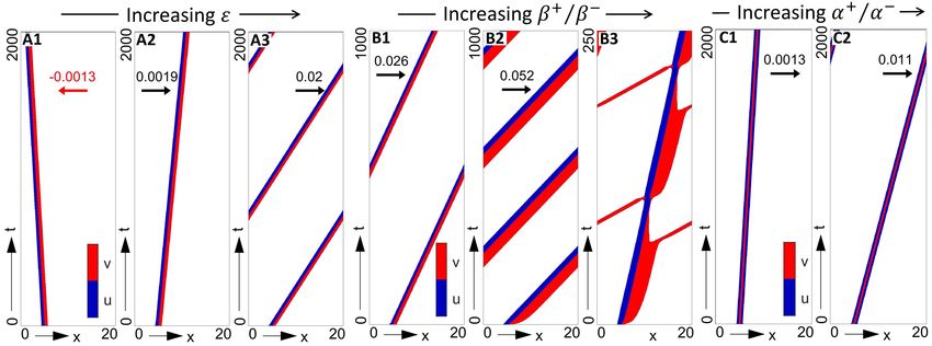
certain destination, finding better environments, hunting or escaping etc. At
the cellular level examples include epithelial wound healing, where a set of so-
called leader cells at the tissue boundary appear to guide a migrating cell group
[37], embryonic neural crest cell invasion, where trail-blazing pioneers lead fol-
lowers in the rear [31], and kidney morphogenesis, where the lumen forms as
leading cells leave the epithelialised tube in their wake [2]. Collective invasion of
breast cancer appears to be driven by a specialised population defined by their
expression of basal epithelial genes [8].
    Leadership is also found in various migrating animal groups, for example
arising from a cohort of braver or more knowledgeable individuals: faced by
poor feeding grounds, post-reproductive females take on an apparent leadership
role in the guidance of a killer whale pod, their experience offering a reserve
of ecological knowledge, [5]. As our principal motivation we consider honeybee
swarms, which form as a colony outgrows its nest site. At this point the queen
and two-thirds of the colony depart (leaving a daughter to succeed her) and tem-
porarily bivouac nearby, for example on a tree branch. Over the following hours
to days, a relatively small subpopulation of scout bees (∼ 3 − 5% of the 10,000+
strong swarm) scour the surroundings for a suitable new nest location, poten-
tially several kilometres distant. The quality of a potential site is broadcast to
other swarm members and, once consensus is obtained, the entire colony moves
to the new dwelling. Consequently, guidance of 1000s of naive insects (including
the queen) is entrusted to a relatively small number of informed scouts [32]. Ob-
servations suggest that scouts perform a sequence of high-velocity movements
towards the nest site through the upper swarm [3, 30, 21, 32], “streaking” that
conceivably increases their conspicuousness and communicates the nest direc-
tion.
    Understanding the collective and coordinated dynamics of migrating groups
demands analytical reasoning. The mathematical and computational literature
in this field encompasses a particularly wide range of approaches. Microscopic,
agent-based or individual-based models describe a group as a collection of in-
dividual agents, where the evolution of each particle is tracked over time. Ben-
efiting from their capacity to provide a quite detailed description of an agent’s
dynamics, they offer a relatively natural tool to investigate collective phenomena
(see, for instance, [11, 12, 14, 17, 24, 23, 4]).
    However, as the number of component individuals become large (as would be
typical for many cancerous populations, large animal groups etc), microscopic
methods become computationally expensive and macroscopic approaches may
become necessary. Various continuous models have been proposed to understand
the collective migration dynamics of interacting populations, with nonlocal PDE
frameworks becoming increasingly popular; models falling into this class have
been developed in the context of both ecological and cellular movement, e.g. see
[27, 1, 35, 16, 15]. Their nonlocal nature stems from accounting for the influence
of neighbours on the movements of an individual, and their relative novelty has
also become a source of significant mathematical interest (see [7] for a review).
    The aim of this paper is to investigate the impact of informed leaders on
naive followers, using a nonlocal PDE model that builds on the hyperbolic PDE

                                         2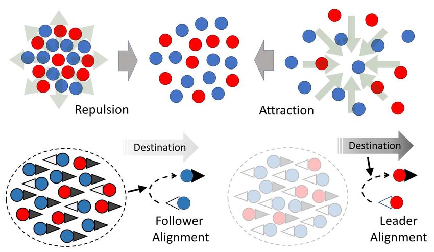
approach developed in [16]. In particular, we will explore the extent to which
the presence of leaders can result in a steered swarm, defined as a population
acquiring and maintaining a spatial compact profile that is consistently steered
towards a target known only to the leaders. Motivated by real-world case stud-
ies (in particular, bee swarming as described above) we assume leaders attempt
to influence the swarm using one or more of three mechanisms: (i) leaders pref-
erentially choose the direction of the target; (ii) leaders move more quickly when
moving towards the target; (iii) leaders alter their conspicuousness according to
the target direction. In Section 2, we introduce the full follower-leader model,
along with two simple submodels – a leader-only and a follower-only system
– designed to reveal insights into the behaviour of the full system. Section 3
explores the dynamics of the submodels, via a combination of linear stability
and numerical simulation. Section 4 subsequently addresses the full system, in
particular the effectiveness of the different biases. We conclude with a discussion
and an outlook of future investigations.

2     Follower-leader swarm model
We assume a heterogeneous swarm composed from distinct populations of knowl-
edgeable leaders and naive followers. Both orient according to their interactions
with other swarm members, as detailed below, but leaders have “knowledge” of
the target and therefore the direction in which the swarm should be steered. For
convenience we will restrict here to one space dimension, assume fixed speeds
and account for direction through separately tracking positively (+) and neg-
atively (−) oriented populations. Without loss of generality we assume the
leaders aim to herd the swarm in the (+) direction, influencing via:
    • Bias 1, orientation. Leaders preferentially choose the target direction.
    • Bias 2, speed. Leaders alter their speed according to the target direction.
    • Bias 3, conspicuousness. Leaders alter their conspicuousness according
      to the target direction.
   Setting u± (x, t) and v ± (x, t) to respectively denote the densities of followers
and leaders at position x ∈ Ω ⊂ R and time t ∈ [0, ∞), the governing equations

                                         3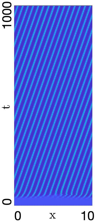
are as follows:
                     ∂u+       ∂u+                  +           −
                          +γ           =       −λu u+ + λu u− ,
                      ∂t        ∂x
                     ∂u−       ∂u−                  +           −
                          −γ           =       +λu u+ − λu u− ,
                      ∂t        ∂x
                    ∂v +       ∂v +                 +           −
                         + β+          =       −λv v + + λv v − ,
                     ∂t         ∂x
                       −
                    ∂v         ∂v −                 +           −
                         − β−          =       +λv v + − λv v − ,
                     ∂t         ∂x
                          u± (x, 0)    =       u±0 (x) ,
                          v ± (x, 0)   =       v0± (x) .                       (1)
In its general setting the model is formulated under the assumption of an infinite
1D line. For the simulations later we consider a bounded interval Ω = [0, L], but
wrapped onto the ring (periodic boundary conditions) to minimise the influence
of boundaries. Initial conditions will be specified later.
    In the above model, followers move with a fixed speed (set at γ). Leaders
have potentially distinct speeds, β± , according to whether bias 2 is in opera-
tion; for example, in the example of bee swarming, scouts engage in streaking
and increase their speed when moving towards the new nest site [32]. Switching
                                                                                 +
between directions is accounted for via the right hand side terms, where λu
denotes the rate at which a follower (u) turns from (+) to (−), with similar def-
                −    ±
initions for λu , λv . Note that the current model excludes switching between
follower and leader status, although it is of course possible to account for such
behaviour through additional role-switching transfer functions.
    The turning rate functions are based on interactions between swarm mem-
bers where, accounting for the “first principles of swarming” [6], we combine
repulsion (preventing collision between swarm members), attraction (preventing
loss of contact and swarm dispersal) and alignment (choosing a direction accord-
ing to those assumed by neighbours and/or external bias). Figure 1 summarises
the general principals upon which the model is founded.
    The turning rate functions have the following form:
                                  ±                     ±
                              λi = λ1 + λ2 f (y i ) ,
for i ∈ {u, v} and where f (y) = 0.5 + 0.5 tanh(y − y0 ). This assumes the turning
rate smoothly and monotonically increases from a baseline to maximum value
according to the level of perceived signal, measured separately for (+) and (−)
                                       ±         ±
follower and leader populations in y u and y v . If y0 is chosen in such a way
that f (0) ≪ 1 the coefficients λ1 and λ2 can be regarded as the baseline turning
rate and the highly biased turning rate respectively. For positively-moving fol-
                                    +
lowers at position x and time t, y u (x, t) combines the repulsive, attractive and
alignment interactions with their neighbours into a single measure that dictates
                                                       −    ±
the turning rate, with similar interpretations for y u , y v . Specifically, we set
                              ±        ±           ±        ±
                            y u = Qur + Qua + Qul                              (2)

                                           4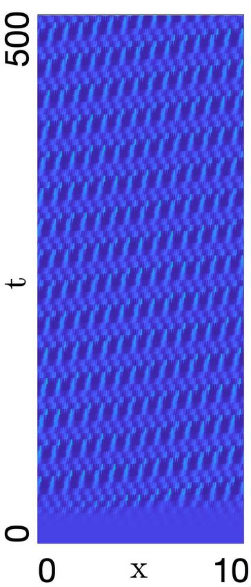
Figure 1: Assumptions underlying the turning behaviour of swarm members.
Top row: attraction and repulsion are assumed to act equally on followers (blue
circles) and leaders (red circles). Repulsion acts over shorter ranges, pushing
individuals away from each other if they are too close; attraction acts over larger
distances, pulling individuals together if they become too separated. Bottom
row: alignment is distinct for followers and leaders. Followers do not know the
target but are influenced by the orientation of the oncoming swarm, reorienting
when they perceive the oncoming swarm is moving in the opposite direction.
Leaders ignore the alignment of the swarm, biasing instead according to the
target direction.

                     ±
and similarly for y v . Qr , Qa and Ql integrate the perceived positional and
directional information from neighbours located at a distance s ∈ (0, ∞) from
the generic individual placed at (x, t).
    For simplicity we will assume here that followers and leaders are only dis-
tinguished by their alignment response: repulsion/attraction are taken as “uni-
versal” and act to keep the overall population together and avoid collisions. A
noteworthy consequence of this is that a leader is not bound to choose the di-
rection of the target: for example, if there is a danger of losing contact with
the swarm the leader should be inclined to return to the fold. We adopt the
following standard choices.
                     Z ∞
    ±      ±
Qur = Qvr      = qr       Kr (s) (u(x ± s) + v(x ± s) − u(x ∓ s) − v(x ∓ s)) ds ,
                      0
                       Z ∞
    ±      ±
Qua = Qva      = −qa        Ka (s) (u(x ± s) + v(x ± s) − u(x ∓ s) − v(x ∓ s)) ds .
                         0

In the above, Ki (s), i = {a, r}, denote interaction kernels and parameters qa

                                        5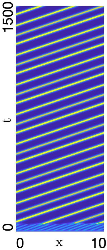
and qr represent the magnitude of the attraction and repulsion contributions,
respectively. The attractive and repulsive terms depend on the total density of
the cohort at a certain position, regardless of flight orientation, i.e. u(x ± s, t) =
u+ (x±s, t)+u− (x±s, t) and similarly v(x±s, t) = v + (x±s, t)+v − (x±s, t). For
an individual flying in the direction of a large swarm (i.e. towards overall higher
total population densities), the contribution to y from Qr will be positive (hence,
an increased likelihood of turning away) and from Qa will be negative (hence
less likely to turn away). Whether the combined contribution is then positive
or negative depends on the individual parameters and the precise shape of the
total density distribution.
    The alignment contribution is of the general form
                                  Z ∞
                          i±
                         Ql = ql       Kl (s)P i (u± , v ± )ds,                    (3)
                                     0

for i ∈ {u, v} and where Kl (s) and ql respectively denote the alignment ker-
nel and the magnitude of the synchronization. The functions P u (u± , v ± ) and
P v (u± , v ± ) respectively represent how the swarm influences alignment for the
follower and leader populations. Choices for Ql , i.e. the specification of P i (u± , v ± ),
form the point of distinction for the various models and are described below, see
Table 1 for a summary of the models interactions. As we will see in Section 2.2,
the latter may simply take into account a fixed preferred direction, i.e. modeling
a case where a population knows where it wants to go.
     Interaction kernels are given by the following translated Gaussian functions

                                     −(s − si )2

                         1
            Ki (s) =           exp                 , i = r, a, l s ∈ [0, ∞),       (4)
                                        2m2i
                      p
                        2πm2i

where sr , sa and sl are half the length of the repulsion, attraction and alignment
ranges, respectively. The constants mi , i = r, a, l, are chosen to ensure > 98%
of the support of the kernel mass falls inside [0, ∞) (specifically, mi = s8i ,
i = r, a, l). This allows a high level approximation of the integral defined on
[0, ∞) to that defined on the whole real line.

2.1    Follower-leader model
The full follower-leader model assumes the following leader alignment
                                 Z ∞
                        ±
                     Qvl = ∓2ql      Kl (s)ε ds = constant                           (5)
                                         0

where we call ε the orientation bias parameter. Leaders ignore other swarm
members for alignment, receiving instead a (spatially uniform and constant)
alignment bias if the orientation bias is operating. Invoking the honeybees
example, scouts have generally agreed on the new nest at swarm take-off. Gen-
eralisations could include letting ε explicitly depend on a variable factor or
including an influence of alignment from other swarm members.

                                             6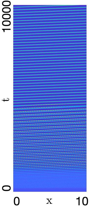
Alignment of followers is taken to be
         Z ∞
   ±
Qul = ql     Kl (s) u∓ (x ± s) + α∓ v ∓ (x ± s) − u± (x ∓ s) − α± v ± (x ∓ s) ds .

           0
                                                                              (6)
This dictates that a follower will be more likely to turn when it detects, within
the region into which is moving, a large number of individuals moving in the
opposite direction. Other plausible choices can be considered, however we choose
the present form for its consistency with that assumed in [16]. Note that α± are
weighting parameters that distinctly weight the leader conspicuousness, bias 3.
Completely inconspicuous leaders would correspond to α± = 0 while if leaders
are completely indistinguishable from followers α± = 1. If leaders engage in
behaviour that raises (lowers) their conspicuousness when flying towards (away
from) the destination we would choose α+ > 1 (α− < 1). For bee swarms,
streaking towards the nest by the scout leaders may serve to increase visibility,
while “laying low” on return may decrease it [32].

2.2     100% leader model
A leader-only model can be obtained by setting follower populations to zero
(u± (x, t) = 0). As noted, attraction/repulsion social interactions are main-
tained, but the alignment bias is independent of the population. The target
direction is potentially favoured through bias 1 (ε) and bias 2 (β+ 6= β− ,
differential speeds). The model reduces to
                    ∂v +       ∂v +            +         −
                         + β+          = −λv v + + λv v − ,
                     ∂t         ∂x
                    ∂v −       ∂v −            +         −
                         − β−          = +λv v + − λv v − ,
                     ∂t         ∂x
                          v ± (x, 0)   = v0± (x) ,                              (7)
where
    ±
              h                  ±
                                        i          ±     ±     ±     ±
  λv = λ1 + λ2 0.5 + 0.5 tanh(y v − y0 ) , with y v = Qvr + Qva + Qvl .

The interaction contributions are given by
                           Z ∞
                  ±
              Qvr   = qr        Kr (s) (v(x ± s) − v(x ∓ s)) ds ,               (8)
                            0
                             Z ∞
                  ±
              Qva   = −qa         Ka (s) (v(x ± s) − v(x ∓ s)) ds ,             (9)
                              0
                              Z ∞
                  ±
              Qvl   = ∓2ql        Kl (s)εds = constant .                       (10)
                                0

2.3     100% follower model
We obtain a follower-only model by ignoring dynamic evolution of the leaders.
Specifically, we stipulate fixed and uniform leader populations, i.e. v + (x, t) and

                                         7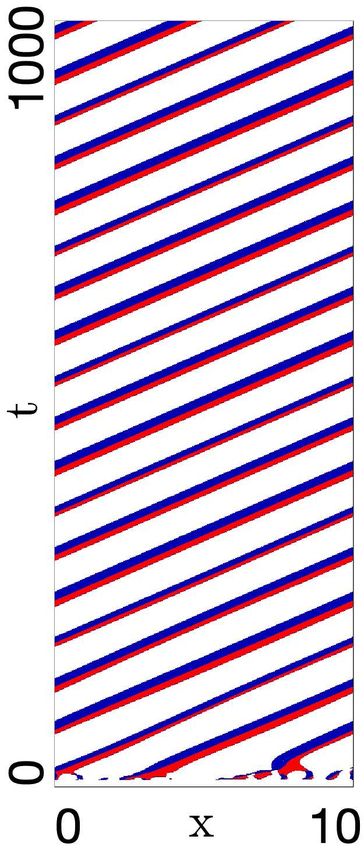
Table 1: Summary of the interactions involved in the models. “Full” denotes
Full follower-leader model; “LO” denotes Leaders Only model; “FO” denotes
Followers Only model.

                                               Full                       LO              FO

 Pop. composition            Leaders (L)          Followers (F)       Leaders (L)   Followers (F)

 Attraction to               F+L                  F+L                 F+L           F+L

 Repulsion to                F+L                  F+L                 F+L           F+L

 Alignment to                implicit             F+L                 implicit      F + implicit
                             orientation          (weighted           orientation   leader
                             bias ε               with α± )           bias ε        bias η

v − (x, t) are constant in space and time. A leader contribution to attraction and
repulsion is eliminated while their contribution to follower alignment is reduced
to a fixed and constant bias, which we refer to as an implicit leader bias and
represent by parameter η: large η corresponds to highly influential leaders. The
resulting model is given by
                    ∂u+      ∂u+                        +         −
                         +γ        =               −λu u+ + λu u− ,
                     ∂t       ∂x
                       −        −
                    ∂u       ∂u                         +         −
                         −γ        =               +λu u+ − λu u− ,
                     ∂t       ∂x
                         u± (x, 0) =               u±
                                                    0 (x) ,                               (11)
where
    ±
              h                  ±
                                        i          ±     ±     ±     ±
  λu = λ1 + λ2 0.5 + 0.5 tanh(y u − y0 ) , with y u = Qur + Qua + Qul .

and interaction terms
                             Z       ∞
               ±
            Qur    =    qr               Kr (s) (u(x ± s) − u(x ∓ s)) ds ,                (12)
                                 0
                             Z ∞
               ±
            Qua    =    −qa      Ka (s) (u(x ± s) − u(x ∓ s)) ds ,                        (13)
                           Z ∞0
               ±
            Qul                 Kl (s) u∓ (x ± s) − u± (x ∓ s) ∓ η ds .

                   =    ql                                                                (14)
                              0

2.4     Parameters
Given its complexity, the model has a large parameter set and we therefore
fix many at standard values, based on previous studies [16] and listed in Ap-

                                                   8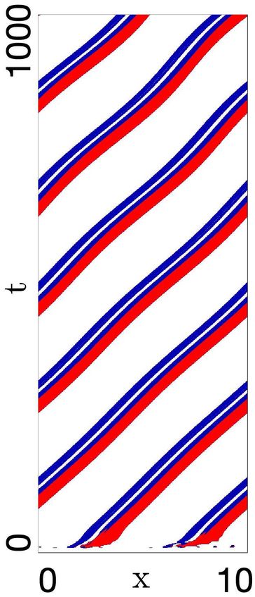
Table 2: Table of parameters varied throughout this study. The parameters
that are fixed throughout this study are summarised in Table 3 (see Appendix
A). “LO” denotes Leaders Only model; “FO” denotes Followers Only model.

 Grouping       Parameter                     Description                    Model

 Bias:          α+              alignment due to (+) oriented leaders       Full
                α−              alignment due to (−) oriented leaders       Full
                η               implicit leader bias                        FO
                ε               implicit orientation bias                   LO, Full
                β+              speed of (+) moving leaders                 LO, Full
                β−              speed of (−) moving leaders                 LO, Full

 Pop. size:     Au              mean follower density                       FO, Full
                Av              mean leader density                         LO, Full
                Mu              maximum initial follower density            Full
                Mv              maximum initial leader density              Full

 Interaction:   qr              repulsion strength                          All
                ql              alignment strength                          All
                qa              attraction strength                         All

 Others:        λ1              baseline turning rate                       All
                λ2              bias turning rate                           All

pendix A. The fixed parameters include the follower speed γ as well as the
interaction ranges sr , sl , sa , fixed to generate “short-range repulsion, mid-range
alignment and long-range attraction”, a common assumption in biological mod-
els of swarming behaviour [33, 6, 17]. Similarly, the more technical parameters
y0 , ml , ma , mr are also chosen according to [16], see Appendix A.
     Consequently, we focus on a smaller set of key parameters that distinguish
leader/follower movement, listed in Table 2 along with the models to which
they belong. In particular, we highlight the bias parameters that stipulate a
level of attempted leader influence. We also remark that model formulations
lead to conservation of follower and leader populations, generating two further
population size parameters. As a final note, we generally restrict to alignment-
attractive dominated regimes, i.e. qa , ql ≫ qr .

                                         9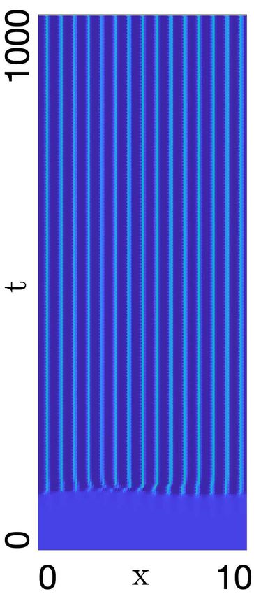
3       Dynamics of Leaders Only and Followers Only
        models
We first analyse the dynamics of the simplified models, via linear stability anal-
ysis and numerical simulation. Note that details of the numerical scheme are
provided in Appendix B.

3.1     100% leader model
In this model, all swarm members have some knowledge of their target and bias
their movement through two mechanisms: bias 1, orientation according to the
target and parametrised by ε ≥ 0, and bias 2, differential speed of movement,
i.e. β+ ≥ β− .

3.1.1    Steady states and stability analysis
We first examine the form and stability of spatially homogeneous steady state
(HSS) solutions, v + (x, t) = v ∗ and v − (x, t) = v ∗∗ , for the leader-only model
(7-10). Conservation of mass leads to Av = v ∗ + v ∗∗ , where Av is the sum of
initial population densities averaged over space (Av = v0+ (x) + v0− (x) ). The
steady state equation is obtained by solving

                               h(v ∗ , ql , λ, Av , ε) = 0,                     (15)

where

           h(v ∗ , ql , λ, Av , ε) = −v ∗ (1 + λ tanh(−2εql − y0 ))
                                     +(Av − v ∗ )(1 + λ tanh(2εql − y0 ))

and
                                           0.5λ2
                                  λ=               .                            (16)
                                        0.5λ2 + λ1
From Eq. 15, we obtain a single HSS solution

                                Av [1 + λ tanh(2εql − y0 )]
                v∗ =                                                .           (17)
                       2 + λ tanh(−2εql − y0 ) + λ tanh(2εql − y0 )

For ql = 0 (no alignment)         or ε = 0 (no bias 1) we obtain an unaligned HSS
(v ∗ , v ∗∗ ) = A2v , A2v , i.e. a population equally distributed into those moving


in (±) directions. Assuming ε > 0, dominating alignment (ql → ∞) leads to
steady state (v ∗ , v ∗∗ ) = (Av (1 + λ)/2, Av (1 − λ)/2). For ql > 0 the same result
follows for dominating bias 1, i.e. ε → ∞. Intuitively, the introduction of bias
eliminates symmetry, with ε > 0 tipping the balance into a (+) direction, with
alignment amplifying the effect. The steady state variation with ε is illustrated
in Figure 2A. Unlike bias 1, introduction of differential leader speed does not
alter the HSS solution, since h does not depend on β± , see Figure 2B.

                                           10
To assess stability and the potential for pattern formation we perform a stan-
dard linear stability analysis. Specifically, we examine the growth from homoge-
neous and inhomogeneous perturbations of the HSS at (v ∗ , v ∗∗ ) = (v ∗ , Av − v ∗ ).
Note that here it is convenient to extend Kr and Ka to odd kernels on the whole
real line, i.e.
Z +∞
±
Qvr = qr Kr (s)v(x ± s)ds,
−∞
Z +∞
±
Qva = −qa Ka (s)v(x ± s)ds.
−∞
We set v + (x, t) = v ∗ + vp (x, t) and v − (x, t) = v ∗∗ + vm (x, t), where vp (x, t)
and vm (x, t) each denote small perturbations. We substitute into (7), neglect
non-linear terms in vp and vm and look for solutions vp,m ∝ eσt+ikx . Here, k
is referred to the wavenumber (or spatial eigenvalue) while σ is the growth rate
(or temporal eigenvalue). A few rearrangements lead to the expression
p
+ C(k) + C(k)2 − D(k)
σ (k) = , (18)
2
where σ + (k) is used to denote the growth rate with largest real part. In the
above
C(k) = (β− − β+ )ik − 2λ1 − λ2 − 0.5λ2 [tanh(−2ql ε − y0 ) + tanh(2ql ε − y0 )] ,
D(k) = 4β+ β− k 2 + 4ikλ1 (β+ − β− )
+2λ2 ik{β+ (1 + tanh(2ql ε − y0 )) − β− (1 + tanh(−2ql ε − y0 ))
+v ∗ [1 − tanh2 (−2ql ε − y0 )][(−qr K̂r+ (k) + qa K̂a+ (k))(β+ + β− )]
+v ∗∗ [1 − tanh2 (2ql ε − y0 )][(qr K̂r− (k) − qa K̂a− (k))(β+ + β− )]},
where K̂j± (k), j = r, a, l denote the Fourier transform of the kernel Kj (s), i.e.
+∞
k 2 m2l
Z
K̂j± (k) = Kj (s)e±iks ds = exp ±isj k − , j = r, a, l.
−∞ 2
The HSS is unstable (stable) to homogeneous perturbations if ℜ(σ + (0)) > 0
(ℜ(σ + (0)) ≤ 0) and unstable to inhomogeneous perturbations if ℜ(σ + (k)) > 0
for at least one valid k > 0 (for an infinite domain, we simply require ℜ(σ + (k)) >
0 for at least one value of k ∈ R+ ). Any k for which ℜ(σ + (k)) > 0 is referred
to as an unstable wavenumber.
We classify HSS stability according to the following principle forms:
(S1) Unstable to homogeneous perturbations, i.e. ℜ(σ + (0)) > 0. Solutions are
expected to diverge from the HSS both with and without movement.
(S2) Stable to homogeneous and inhomogeneous perturbations, i.e. ℜ(σ + (k)) <
0, ∀k ≥ 0. We expect small (homogeneous or inhomogeneous) pertur-
bations to decay and solutions that evolve to the HSS.
11(S3) Stationary patterns, HSS stable to homogeneous perturbations and unsta-
ble to inhomogeneous perturbations. Specifically, we have ℜ(σ + (0)) ≤ 0
but ∃k̃ > 0 : ℜ(σ + (k̃)) > 0 where, for any such k̃, ℑ(σ + (k̃)) = 0.
(S4) Dynamic patterns, as (S3), but ℑ(σ + (k̃)) 6= 0 for at least some of the
unstable wavenumbers.
(S3) and (S4) both indicate a Turing-type instability [36], i.e. symmetry break-
ing in which a spatial pattern emerges from quasi-homogeneous initial condi-
tions. The presence of wavenumbers where ℑ(σ + (k̃)) 6= 0 implies growing pat-
terns that oscillate in both space and time, potentially generating a dynamic
pattern (e.g. a travelling swarm). These are, though, predictions based on so-
lutions to the linearised system and nonlinear dynamics are likely to introduce
further complexity.
Key results from the analysis are summarised in Figure 2, indicating that
both the HSS and its stability change with bias parameters ε (or ql ), the ra-
tio β+ /β− and qa . As noted above, increasing ε (or ql ) generates a HSS with
(±) distributions increasingly favouring the target direction. Variations in the
β+ /β− ratio do not alter the HSS value but do impact on the stability. Un-
der both biases 1 and 2, the stability nature changes at key threshold values,
critically depending on the strength of attraction, qa . For low qa the HSS is
stable for all values of ε and/or β+ /β− : attraction is insufficient to cluster the
population and it remains dispersed. There may be biased movement towards
the target, but the population remains in a uniformly dispersed/non-swarming
state.
For larger qa , however, the HSS becomes unstable under inhomogeneous
perturbations. A Turing-type instability occurs and emergence of a spatial
pattern is expected. The predicted pattern critically depends on the bias. For an
unbiased scenario (ε = 0 and β+ /β− = 1) we have stability class (S3) and predict
a stationary pattern, see dark green asterisks in Figures 2A and 2B. Simulations
corroborate this prediction (see Figure 2C), where we observe stationary cluster
formation. Each cluster is weighted equally between (±) directed populations
and the overall cluster is fixed in position. Note, however, that the nonlocal
elements of the model generate a degree of intercluster communication and,
over longer timescales, clusters may attract each other and merge.
Introducing bias 1 (ε > 0) or bias 2 (β+ /β− > 1), though, generates growth
rates with imaginary components – this follows from the nonzero imaginary
parts of D(k) and/or C(k) – and the instability is of type (S4). In this case
a dynamic component is predicted, with simulations substantiating this, cf.
Figures 2D and 2E. The forming clusters are asymmetrically distributed between
(±) directed movement and, overall, we observe steered swarming: clusters move
in the direction determined by the bias. Notably, clusters move at distinct speeds
according to their size, so that clusters collide and merge. Eventually, a single
steered swarm has formed and migrates with fixed speed and shape (a travelling
pulse). The simultaneous action of biases 1 and 2 generates similar behaviour,
Figure 2F, with the combined action creating faster movement towards the
target.
12Figure 2: Dynamics of the leader-only model. (A-B) Bifurcation plots showing
HSS (proportion moving rightwards) and stability under parameter variation.
(A) Bias 1, i.e. variation of ε under low (top panel, qa = 0.5) and high (bottom
panel, qa = 50) attraction (bias 2 inactive, β+ = β− = 0.1). (B) Bias 2,
varying β+ for fixed β− = 0.1, under low (top panel, qa = 0.5) and high (bottom
panel, qa = 50) attraction (bias 1 inactive, ε = 0). Solid blue and dashed black
lines denote stability class S2 and S4 respectively, dark green asterisks indicate
stability class S3. (C-F) Space-time density map showing evolving total leader
density, under: (C) unbiased case, generating a stationary patterns; (D) bias 1,
obtained for ε = 0.2 (bias 2 inactive, β+ = β− = 0.1), generating target directed
swarms; (E) bias 2, obtained for β+ /β− = 0.2/0.1 (bias 1 inactive, ε = 0),
generating target directed swarms; (F) biases 1 and 2, obtained for ε = 0.2
and β+ /β− = 0.2/0.1, generating target directed swarms with enhanced speed.
(C-F) ICs are perturbations of (v ∗ , v ∗∗ ) = (2, 2). (D) ICs are perturbations of
(v ∗ , v ∗∗ ) = (3.329, 0.671). In all plots, other parameters are set at qr = 0.1,
ql = 7.5, ((C-F) qa = 7.5), Av = 4, λ1 = 0.2, λ2 = 0.9.
Summarising, the leader-only model illustrates the distinct contributions
from different model elements: (i) attraction is crucial to aggregate a dispersed
population; (ii) assuming sufficient attraction, either bias 1 or bias 2 is suffi-
cient to propel the swarm in the direction of the target, with increased swarm
speed if both biases act together.
3.2 100% follower model
We next examine the follower-only model. Interaction occurs through attrac-
tion, repulsion and alignment, with an additional uniform alignment bias parametrised
by η and corresponding to implicit perception of a leader population.
3.2.1 Steady states and stability analysis
Proceeding as before, we explore the form of spatially homogeneous steady state
solutions. Conservation of the total follower population leads to Au = u∗ + u∗∗ ,
13where Au is the average (over space) of the sum of initial population densities,
Au = u+ −
0 (x) + u0 (x) . Steady states will be given by
h(u∗ , ql , λ, Au , η) = 0, (19)
where
h(u∗ , ql , λ, Au , η) = −u∗ (1 + λ tanh(Au ql − 2u∗ ql − ηql − y0 ))
+(Au − u∗ )(1 + λ tanh(−Au ql + 2u∗ ql + ηql − y0 ))
and
0.5λ2
λ= . (20)
0.5λ2 + λ1
The zero-bias scenario (η = 0) has been analysed in depth previously, see
[16], and we restrict to a brief summary. First, a single unaligned HSS exists at
Au Au
(u∗ , u∗∗ ) = ( , ),
2 2
i.e. both directions equally favoured. Dominating alignment (ql → ∞) generates
two further HSS at (u∗ , u∗∗ ) = (Au (1 ∓ λ)/2, Au (1 ± λ)/2): each aligned HSS
corresponds to a population where alignment induces the population to favour
one direction. A typical structure for the bifurcation diagram is illustrated in
Figure 3A: a central branch corresponding to the unaligned HSS and upper
and lower aligned branches. For the chosen parameters, these branches are
connected via a further set of intermediate (unstable) branches. Thus, as ql
increases the number of steady states shifts between 1, 5 and 3 steady states
(see also Figure 10 of Appendix C.2).
The symmetric structure of η = 0 is lost for η 6= 0, even under small val-
ues: see Figures 3B-C. The aligned HSS branch corresponding to the target
direction is more likely to be selected, the other branch is shifted rightwards
(Figure 3B) and for larger η disappears entirely (Figure 3C). Overall, the ex-
ternal bias is amplified by follower to follower alignment and the population
becomes predominantly oriented in the target direction.
We extend to a spatial linear stability analysis, applying the same process
as in section 3.1.1 to obtain the following dispersion relation
p
C(k) + C(k)2 − D(k)
σ + (k) = , (21)
2
where
+ +
− −
− +
C(k) = λuu− − λuu+ u+ + λuu+ − λuu− u− − λu − λu , (22)
D(k) = 4γ 2 k 2
h + +
− −
− +
i
+4γik −λuu− − λuu+ u+ + λuu− + λuu+ u− + λu − λu .(23)
± ±
In the above, λuu± denote the partial derivatives of λu with respect to u±
and subsequently evaluated at the HSS (u∗ , u∗∗ ). For reference we provide the
14explicit forms in Appendix C.1, yet intricacy of the dispersion relation restricts
us to a numerical approach. Stability is again classified into one of the 4 classes
described earlier.
The diagrams shown in Figure 3A-C reveal a complex bifurcation structure
and potentially diverse dynamics according to parameter selection and initial
condition. Indeed, this has already been highlighted in depth for the unbiased
(η = 0) model in [16], where various complex spatiotemporal pattern forms have
been revealed. For example, Figure 11 in Appendix C.3 illustrate transitioning
between stationary and dynamic aggregates as the key parameter ql is altered.
Note that moving aggregates can be generated without any incorporated bias,
though if the population begins quasi-symmetric either direction will be selected
with equal likelihood.
Here we focus on the extent to which introduction of a bias influences the
dynamics of aggregate structures, with Figure 3D-G providing a representative
sequence. We begin with an unbiased scenario, setting η = 0 and choosing
parameters from a region predicted to lead to stationary patterning. We initiate
populations in quasi-symmetric fashion, setting
Au (1 + ru (x)) Au (1 − ru (x))
u+ (x, 0) = , u− (x, 0) = ,
2 2
where ru (x) denotes a small random perturbation. As expected from the sta-
bility analysis, a stationary cluster forms (see Figure 3D) with its shape and
position maintained by a symmetric distribution of (±) directed populations. In-
troducing bias, though, disrupts the symmetry and Turing instabilities falls into
the dynamic pattern class. Moreover, even a marginal alignment bias strongly
selects clusters that move in the direction of the bias, e.g. see Figures 3E. Start-
ing from a symmetric or nonaligned initial set-up, bias slightly tilts followers
towards the target. Follower-follower alignment snowballs, eventually resulting
in a cluster moving towards the target. Increasing the bias magnitude increases
swarm speed, Figure 3F.
As for the 100% leader model, there is a clear relationship between cluster
speed and cluster size. This is illustrated in Figure 3G, where the initial sym-
metry breaking process generates two clusters of slightly different size, Figure
3H(bottom). Both clusters move in the target direction, but the smaller cluster
is considerably faster. The clusters eventually collide and merge to form an
even larger and slower cluster, see Figure 3H(top). Note that, in principle it is
also possible to obtain a swarm migrating oppose the target direction, e.g. by
heavily favouring biasing the initial conditions. Simulations, though, suggest
that such situations are highly unlikely to occur in practice.
Introducing bias can even trigger symmetry breaking, as shown in Figure 4.
To highlight this, we neglect attractive and repulsive interactions (qa = qr = 0)
and focus solely on alignment. Initially setting η = 0, remaining parameters
are specified such that the unaligned HSS (i.e. u∗ = u∗∗ ) is stable to both
homogeneous and inhomogeneous perturbations: a typical dispersion relation is
provided in Figure 4A (top), showing the absence of wavenumbers with positive
growth rates and the corresponding simulation confirms the absence of pattern
15Figure 3: Dynamics of the follower-only model. (A-C) Bifurcation plots showing
HSS (proportion moving rightwards) and stability under parameter variation.
Bifurcation parameter is ql and the resulting bifurcation plots are shown for
(A) η = 0 (unbiased), (B) η = 0.04, (C) η = 4. Other parameters set at
qr = 0, qa = 0.25, Au = 2, λ1 = 0.8, λ2 = 3.6. Stability classes plotted as S1:
dotted red, S2: solid blue, S3: dark green asterisks, S4: dashed black. (D-F)
Space-time plot showing the evolving total follower density under variation of
η: (D) η = 0 (unbiased), (E) η = 0.04, (F) η = 4. Stronger biases lead to
faster swarm movement towards the target. Other parameters set as in (A-
C) with ql = 0.4. ICs are perturbations of (u∗ , u∗∗ ) = (1, 1). In (G-H) we
demonstrate the merging of faster and slower swarms, under the parameter set
η = 0.4, qr = 0.1, ql = 1, qa = 10, Au = 2, λ1 = 0.2, λ2 = 0.9.
16Figure 4: (A) Dispersion relations and (B-C) the corresponding numerical simu-
lations for the following parameter values: qr = 0, ql = 2.1, qa = 0, Au = 2, λ1 =
0.8, λ2 = 3.6. (A) top row and (B) assume no bias (η = 0), while (A) bottom
row and (C) consider the effect of a small alignment bias (η = 0.08). (B-C) ICs
are perturbations of (u∗ , u∗∗ ) = (1,1).
formation, Figure 4B. Introducing bias (η > 0) breaks symmetry, yielding a
nonzero range of wavenumbers with positive growth rates, Figure 4A (bottom).
A pattern emerges which generates multiple clusters moving in the target direc-
tion, Figure 4C.
Summarising the analysis and numerics in this section, we emphasize that the
follower only submodel can display a range of aggregating/swarming behaviour,
where the processes of alignment and attraction combine to generate one or
more cluster. The addition of bias breaks directional symmetry, eliminating the
formation of stationary structures and generating clusters that move coherently
in the target direction.
4 Dynamics of the full follower-leader model
We turn attention to the full “follower-leader” model, formed from Equations
(1-6) and where followers constitute a completely naive population. Our prin-
cipal aim will be to understand whether a steered swarm can arise under leader
generated bias. Relying principally on numerical simulation, we focus on two
general parameter regimes: (P1) strong attraction-strong alignment, and (P2)
strong attraction-weak alignment. For simplicity we neglect repelling interac-
tions (qr = 0). A bias corresponding to the (+)-direction can occur through
17parameter choices:
• Bias 1, ε > 0, orientation;
• Bias 2, β+ > β− , speed;
• Bias 3, α+ > α− , conspicuousness.
Consequently, the unbiased case is ε = 0, α+ = α− , and β+ = β− . As discussed
earlier, evidence is found for each bias in our honeybee swarming exemplar.
Note that parameter regimes are selected such that linear stability analysis of
the uniform solution in the unbiased case predicts Turing pattern formation.
4.1 Steady state analysis
Steady state analysis proceeds as before: we look for the spatially homogeneous
steady states u+ (x, t) = u∗ , u− (x, t) = u∗∗ and v + (x, t) = v ∗ , v − (x, t) = v ∗∗ ,
noting that conservation ensures Au = u∗ + u∗∗ and Av = v ∗ + v ∗∗ , where Au
and Av are as earlier described. Steady states for the full model satisfy
hu (u∗ , ql , λ, Au , Av , α− , α+ , y0 ) = 0, (24)
∗
hv (v , ql , λ, Av , ε, y0 ) = 0, (25)
where
hu = −u∗ (1 + λ tanh(Au ql − 2u∗ ql + ql α− (Av − v ∗ ) − ql α+ v ∗ − y0 ))
+(Au − u∗ )(1 + λ tanh(−Au ql + 2u∗ ql + ql α+ v ∗ − ql α− (Av − v ∗ ) − y0 )),
hv = −v ∗ (1 + λ tanh(−2εql − y0 )) + (Av − v ∗ )(1 + λ tanh(2εql − y0 )),
and
0.5λ2
λ= . (26)
0.5λ2 + λ1
Leader steady states correspond to those obtained previously for the leader-only
model. Hence, the proportion of leaders at HSS moving in the (+) direction
increases monotonically between Av /2 and Av (1+λ)/2, according to ε and/or ql ,
(Figure 2A). This equivalence stems from the simplification that leaders ignore
others with respect to alignment.
In absence of alignment, i.e. ql = 0, we find a single unaligned HSS at
(u∗ , u∗∗ , v ∗ , v ∗∗ ) = (Au /2, Au /2, Av /2, Av /2). If ql 6= 0, follower steady states
are clearly more complex and we first consider the unbiased case (ε = 0, α+ =
α− , β+ = β− ). Here we have v ∗ = v ∗∗ = Av /2 and hence
hu = −u∗ (1 + λ tanh(Au ql − 2u∗ ql − y0 ))
+(Au − u∗ )(1 + λ tanh(−Au ql + 2u∗ ql − y0 )) .
Leaders have no influence and follower steady states are as observed for the
follower-only model with η = 0. As described earlier, the number of follower
steady states varies between 1, 3 and 5 (see Figure 10 of the Appendix C.2) with
18sufficiently large alignment allowing followers to self-organise into a dominating
orientation.
We next consider an extreme bias 1 (ε → ∞), while excluding other bi-
ases (α = α+ = α− , β+ = β− ). Leaders favour the (+) direction, specifically
(v ∗ , v ∗∗ ) = ( Av (1+λ)
2 , Av (1−λ)
2 ), and hence
hu = −u∗ (1 + λ tanh(Au ql − 2u∗ ql − ql αAv λ − y0 ))
+(Au − u∗ )(1 + λ tanh(−Au ql + 2u∗ ql + ql αAv λ − y0 )) .
The above has the same structure as for the follower-only model under external
bias, where η in Equation (19) is replaced by αAv λ. Consequently, for either
increasing leader to follower influence (α) or increasing leader population size
(Av ), bifurcations occur as in Figure 3A-C: symmetric follower steady states
become asymmetric, favoured according to the bias.
Differential speeds (bias 2, β+ 6= β− ) do not impact on steady states and we
turn instead to distinct conspicuousness, specifically extreme bias 3 (α+ /α− →
∞) while eliminating bias 1. Leader steady states remain symmetrical (v ∗ =
v ∗∗ = Av /2), yet distinct conspicuousness tips the majority of followers to the
bias direction and a single steady state occurs at
(u∗ , u∗∗ , v ∗ , v ∗∗ ) = (Au (1 + λ)/2, Au (1 − λ)/2, Av /2, Av /2) .
The bifurcation diagrams in Figure 5 numerically confirm these results. Finally,
we note that as ql → ∞ two further HSS’s arise at (u∗ , u∗∗ , v ∗ , v ∗∗ ) = (Au (1 ∓
λ)/2, Au (1 ± λ)/2, Av (1 + λ)/2, Av (1 − λ)/2).
4.2 Numerical simulation
The steady state analysis provides insight into whether different biases induce
left-right asymmetry, yet the emerging dynamics of spatial structures remains
unclear. We numerically explore the full spatial nonlinear problem, in particular
its capacity to generate a steered swarm as described earlier. Simulations will
be conducted for two forms of initial condition.
(IC1) Unbiased and dispersed. Populations quasi-uniformly distributed in space
and orientation. Letting Au and Av , respectively denote the mean total
follower and leader densities,
Au (1 + ru (x)) Au (1 − ru (x))
u+ (x, 0) = , u− (x, 0) = ,
2 2
Av (1 + rv (x)) Av (1 − rv (x))
v + (x, 0) = , v − (x, 0) = .
2 2
(IC2) Unbiased and aggregated. Populations initially aggregated but unbiased in
orientation. Letting Mu and Mv respectively denote the maximum initial
19Figure 5: Proportion of right-moving populations at steady state(s). (A,C)
Effect of bias 1, increasing ε, on position and number of equilibrium points
(bias 2 and 3 inactive, β− = β+ = 0.1, α− = α+ = 1). (B,D) Effect of bias 3,
increasing α+ /α− , on position and number of equilibrium points, for α− = 0.2
(bias 1 and 2 inactive, ε = 0 and β− = β+ = 0.1). Top row corresponds to
(P1) strong attraction-strong alignment (qr = 0, ql = 10, qa = 8), bottom row
corresponds to (P2) strong attraction-weak alignment (qr = 0, ql = 1, qa = 10).
Other parameter values fixed at Au = Av = 1, λ1 = 0.2, λ2 = 0.9.
20-
Figure 6: Dynamics of the full-model, unbiased case, obtained for ε = 0, β− =
β+ = 0.1, α− = α+ = 1. (A,C) Space-time evolution of densities under (IC1)
for (A) P1, strong attraction-strong alignment, (C) P2, strong attraction-weak
alignment. Non-white regions indicate where the total population > 2(Au +Av ),
i.e. “clustering” has occurred, with red/blue indicating local predominance of
leaders/followers respectively. Panels (B,D) show (top) population distribution
and (bottom) population fluxes for solutions under (IC2) for (B) P1, strong
attraction-strong alignment, (D) P2, strong attraction-weak alignment. (P1)
qr = 0, ql = 10, qa = 8, (P2) qr = 0, ql = 1, qa = 10, with other parameter value
set as Au = Av = 1 (IC1), Mu = Mv = 12.61 (IC2), λ1 = 0.2, λ2 = 0.9.
follower and leader densities,
2 2
Mu e−5(x−x0 ) (1 + ru (x)) Mu e−5(x−x0 ) (1 − ru (x))
u+ (x, 0) = , u− (x, 0) = ,
2 2
2 2
Mv e−5(x−x0 ) (1 + rv (x)) Mv e−5(x−x0 ) (1 − rv (x))
v + (x, 0) = , v − (x, 0) = .
2 2
Note that ru (x), rv (x) denote small (1%) random perturbations. (IC1) allow
investigation into whether dispersed populations self-organise into swarms while
(IC2) tests whether aggregated populations maintain a swarm profile. (IC2) are
particularly appropriate for bee swarming, where followers and leader scouts are
initially clustered together.
4.2.1 Unbiased dynamics
We first explore the capacity for self-organisation in the unbiased scenario. Note
that each of the two principal parameter sets were selected to generate Turing
instabilities and Figure 6A and C demonstrate the patterning process under (P1)
21Figure 7: Impact of biases on swarm movement for the full model in a strong
attraction-strong alignment regime (P1), strong attraction-weak alignment
regime (P2) and under (IC1). Populations plotted in space-time (colourmap as
described in Figure 6). (A,D) Bias 1, obtained for ε = 0.2 (bias 2 and 3 inac-
tive, β− = β+ = 0.1, α− = α+ = 1); (B,E) bias 2, obtained for β+ /β− = 0.5/0.1
(bias 1 and 3 inactive, ε = 0, α− = α+ = 1); (C,F) bias 3, obtained for
α+ /α− = 1.0/0.2 (bias 1 and 2 inactive, ε = 0, β− = β+ = 0.1). Remaining
parameters set at (P1) qr = 0, ql = 10, qa = 8, (P2) qr = 0, ql = 1, qa = 10 and
Au = Av = 1, λ1 = 0.2, λ2 = 0.9.
strong attraction-strong alignment and (P2) strong attraction-weak alignment,
respectively. We observe the formation of multiple swarms which, in the absence
of bias, remain in more or less fixed positions. Note, though, that over longer
timescales inter-aggregate interactions may lead to drifting and merging. The
arrangement and behaviour of an isolated swarm is investigated by initially
aggregating the populations as in (IC2), with reorganisation leading to a stable
and stationary swarm configuration and computed swarm wavespeed c = 0,
Figure 6B and D. Swarms contain leaders1 concentrated at the swarm centre,
with followers symmetrically dispersed either side. The distinct follower/leader
profiles arise as leaders only interact through attraction, while followers receive
additional alignment information. We further plot the fluxes, i.e. the quantities
u+ (x, t) − u− (x, t) and v + (x, t) − v − (x, t). In the stationary swarm profile, (±)
movement is balanced such that the swarm maintains its position and shape,
see Figure 6.
4.2.2 Introduction of leader biases
We perform the same set of simulations, but extended to include one of the
three proposed mechanisms for leader bias. Simulation results under (IC1)
1 These are leaders in name only, as in the unbiased scenario there is no directional bias in
force.
22indicate that self-organisation can be maintained under the inclusion of leader-
bias, where again we observe that an initially dispersed population aggregates
into one or more swarm, see Figure 7. Notably, these swarms can subsequently
migrate through space, indicating that a leader-generated bias can lead to sus-
tained swarm movement. Yet the degree and direction of movement significantly
varies with the type (and strength) of bias, demanding a more extensive analysis
of when and which type of bias leads to steered swarm movement.
To investigate this in a controlled manner, we force populations into form-
ing an isolated swarm by applying (IC2), ensuring that any subsequent swarm
dynamics are the result of internal interactions rather than the influence of
neighbouring swarm profiles. Each of the bias strengths are then progressively
altered, individually or in concert, under each of our two principal parameter
regimes (strong attraction-strong alignment and strong attraction-weak align-
ment): Figures 8 and 9 respectively plot the key behaviours observed for these
two regimes.
The dynamics generated by bias 1 are illustrated in Figure 8A and Figure
9A. Over a wide range of bias strengths, bias 1 generates steered swarming,
with an increased speed in the target direction as ε increases. However two
caveats must be highlighted. First, under certain parameter combinations we
unexpectedly observe swarms that move away from the the target, specifically
for weaker biases in the weak alignment regime (see Figure 9A1). Second,
excessive biases can lead to loss of swarm coherence and eventual dispersion (see
Figure 8A4). Thus, we conclude bias 1 is found to be only partially successful
in generating a steered swarm.
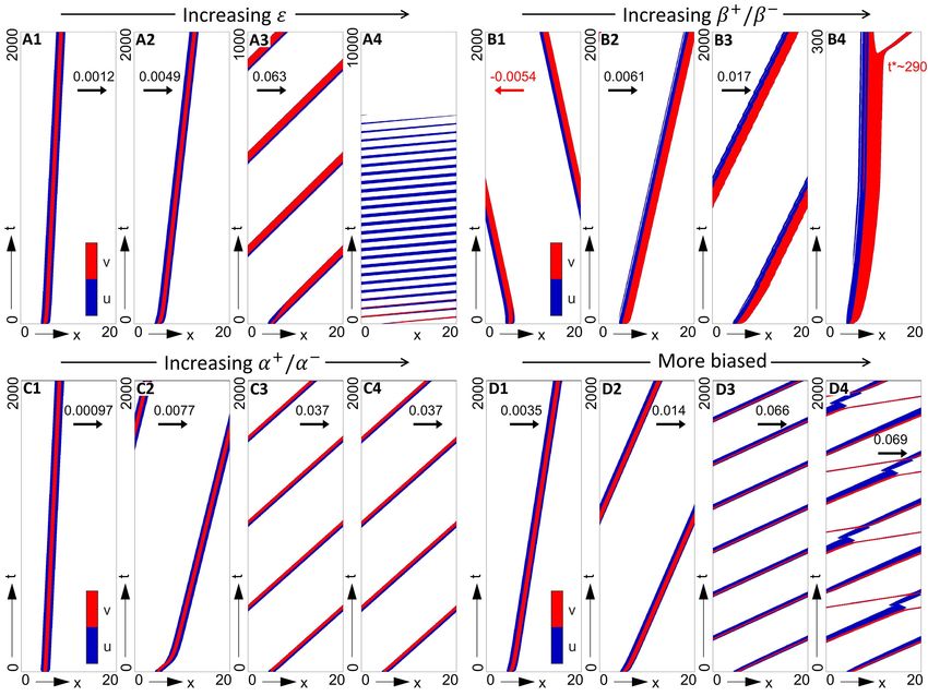
We next consider bias 2, i.e. increasing the ratio of leader speeds when
moving towards or away from the target. Indicative simulations are plotted in
Figures 8B and Figure 9B. Similar to bias 1, successful steering only occurs
within a range of β+ /β− values. First, as observed above under bias 1, certain
parameter regimes are capable of generating counter target directed swarms,
for example see Figure 8B1 for a moderately faster v + population in the high
attraction-high alignment regime. Second, while increasing the speed ratio can
help generate steered swarms, excessively fast target-directed movements can
lead to “swarm-splitting”, i.e. leaders that pull free from followers and leave
them stranded. This phenomenon is observed in Figure 8B4 at around T ≈ 290,
or in Figure 9B3 around T ≈ 80. Under periodic boundary conditions, runaway
leaders eventually reconnect with the stranded followers, leading to a periodic
cycle (see the illustrative example of Figure 9B3). Of course, in a real-world
scenario, leaders would simply leave followers behind.
Representative swarm behaviours under modulation of bias 3, i.e. where
we modulate the relative conspicuous of leaders moving towards or away from
the destination, are shown in Figures 8C and Figure 9C. Notably, this form of
bias was found to consistently generate a steered swarm in the target direction,
over all tested ranges of α+ /α− and for both two parameter regimes.
As a final exploration we examined swarm movement with all biases applied
simultaneously: typical results are shown in Figure 8D for the high attrac-
tion/high alignment regime only. The application of multiple biases appears to
23Figure 8: Impact of biases on swarm movement for the full model in a strong
alignment-strong attraction regime (P1) and under (IC2). Populations plot-
ted in space-time (colourmap as described in Figure 6). Note that we append
each plot with the swarm speed, for cases where a travelling wave solution
is (numerically) found. (A) Bias 1, obtained for ε = (A1) 0.5, (A2) 1.0,
(A3) 2.0, (A4) 3.0 (bias 2 and 3 inactive, β+ = β− = 0.1, α+ = α− = 1).
(B) Bias 2, obtained for β+ /β− = (B1) 0.2/0.1, (B2) 0.3/0.1, (B3) 0.5/0.1,
(B4) 0.6/0.1 (bias 1 and 3 inactive, ε = 0, α+ = α− = 1). (C) Bias 3, ob-
tained for α+ /α− = (C1) 1/0.9, (C2) 1/0.575, (C3) 1/0.55, (C4) 1/0 (bias
1 and 2 inactive, ε = 0, β+ = β− = 0.1). (D) Simultaneous biases, for
(D1) ε = 0.25, β+ /β− = 0.15/0.1, α+/α− = 1/2/3, (D2) ε = 0.5, β+ /β− =
0.2/0.1, α+/α− = 1/0.5, (D3) ε = 0.75, β+ /β− = 0.25/0.1, α+/α− = 1/0.4,
(D4) ε = 1, β+ /β− = 0.3/0.1, α+/α− = 1/(1/3). Other paramenters are (P1)
qr = 0, ql = 10, qa = 8, Mu = Mv = 12.61, λ1 = 0.2, λ2 = 0.9.
reinforce steered movement in the direction of the destination, for example over-
turning the counter-directed swarms obtained for lower ε and ratios of β+ /β− .
Yet escaping leaders can still occur when β+ /β− becomes too large, e.g. see
Figure 8D4.
24Figure 9: Impact of biases on swarm movement for the full model in a strong
attraction-weak alignment regime (P2) and under (IC2). Populations plotted in
space-time (colourmap as described in Figure 6). Note that we append each plot
with the swarm speed, for cases where a travelling wave solution is (numerically)
found. (A) Bias 1, obtained for ε = (A1) 3.0, (A2) 5.0, (A3) 15.0 (bias 2 and 3
inactive, β+ = β− = 0.1, α+ = α− = 1). (B) Bias 2, obtained for β+ /β− = (B1)
0.2/0.1, (B2) 0.8/0.1, (B3) 1/0.1 (bias 1 and 3 inactive, ε = 0, α+ = α− = 1).
(C) Bias 3, obtained for α+ /α− = (C1) 1/0.9, (C2) 1/0 (bias 1 and 2 inactive,
ε = 0, β+ = β− = 0.1). Other parameters are (P2) qr = 0, ql = 10, qa = 8,
Mu = Mv = 12.61, λ1 = 0.2, λ2 = 0.9.
5 Discussion
Collective migration occurs when a population fashioned from interacting indi-
viduals self-organise and move in coordinated fashion. Recently, much attention
has focused on the presence of leaders and followers, essentially a division of the
group into distinct fractions that are either informed and aim to steer or naive
and require steering, [18, 29, 28]. Here we have formulated a continuous model
to understand such phenomena, a non-local hyperbolic PDE system that ex-
plicitly incorporates separate leader and follower populations that have distinct
responses to other swarm members. We considered distinct mechanisms through
which leaders attempt to influence the swarm. Specifically, taking inspiration
from the guidance provided by scout bees, [32, 26], we focused on three different
mechanisms: a bias in the leader alignment according to the target (bias 1),
higher speed (bias 2) when moving towards the target and greater conspicu-
ousness (bias 3) when moving towards the target.
We initially focused on simpler models of greater analytical tractability.
First, a 100% leader model composed only of informed members. Here only
biases 1 or 2 operate, both proving effective at steering the group towards the
destination. Maintaining group cohesion is, unsurprisingly, contingent on suffi-
ciently strong attraction. Second, we considered a 100% follower model: pop-
ulation members were naive but received some alignment bias, e.g. due to an
implicitly present leader population. The range of dynamics generated by this
25You can also read