Adversarial Swarm Defense with Decentralized Swarms - UC ...
←
→
Page content transcription
If your browser does not render page correctly, please read the page content below
Adversarial Swarm Defense with Decentralized
                  Swarms

            Jason Zhou

            Electrical Engineering and Computer Sciences
            University of California, Berkeley

            Technical Report No. UCB/EECS-2021-81
            http://www2.eecs.berkeley.edu/Pubs/TechRpts/2021/EECS-2021-81.html

            May 14, 2021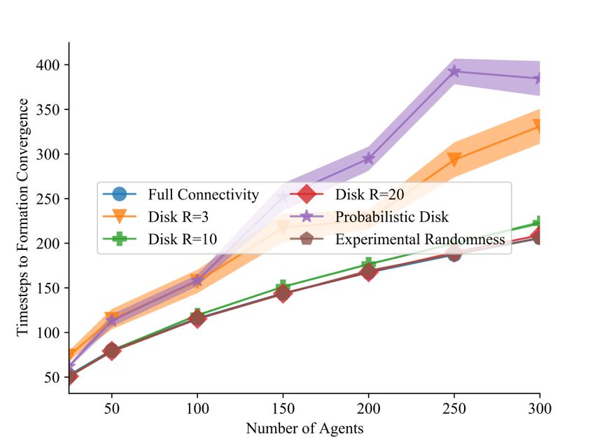
Copyright © 2021, by the author(s).
                            All rights reserved.

Permission to make digital or hard copies of all or part of this work for
personal or classroom use is granted without fee provided that copies are
not made or distributed for profit or commercial advantage and that copies
bear this notice and the full citation on the first page. To copy otherwise, to
republish, to post on servers or to redistribute to lists, requires prior specific
permission.

                               Acknowledgement

I would like to express my deep gratitude to Professor Kris Pister and
Nathan Lambert for their extensive guidance and mentorship throughout
this research process. I am also very grateful to Professor Murat Arcak for
serving as second reader of this thesis. Most of all, I would like to thank my
parents for their unconditional encouragement and support throughout my
entire life.
Adversarial Swarm Defense with Decentralized Swarms

                          by

                   Jason X. Zhou

   A thesis submitted in partial satisfaction of the

            requirements for the degree of

                  Master of Science

                          in

    Electrical Engineering and Computer Sciences

                        in the

                  Graduate Division

                        of the

          University of California, Berkeley

                Committee in charge:

          Professor Kristofer Pister, Chair
              Professor Murat Arcak

                     Spring 2021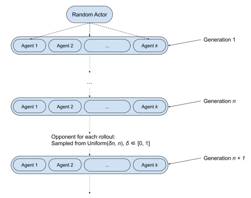
1

                                           Abstract

                   Adversarial Swarm Defense with Decentralized Swarms

                                               by

                                        Jason X. Zhou

            Master of Science in Electrical Engineering and Computer Sciences

                              University of California, Berkeley

                               Professor Kristofer Pister, Chair

The rapid proliferation of unmanned aerial vehicles (UAVs) in both commercial and con-
sumer applications in recent years raises serious concerns of public security, as the versatility
of UAVs allow the platform to be easily adapted for malicious activities by adversarial actors.
While interdiction methods exist, they are either indiscriminate or are unable to disable
a large swarm of drones. Recent work in wireless communications, microelectromechani-
cal systems, fabrication, and multi-agent reinforcement learning make UAV-based counter-
UAV systems increasingly feasible - that is, defense systems consisting of autonomous drone
swarms interdicting intruder drone swarms. Such a system is desirable in that it can con-
ceivably produce a highly versatile, adaptable, and targeted response while still retaining an
aerial presence.
We progress towards such a system through deep reinforcement learning in two distinct do-
mains, which can be broadly described as 1-vs-1 and N-vs-N autonomous adversarial drone
defense. In the former scenario, we learn reasonable, emergent drone dogfighting policies us-
ing soft actor-critic through 1-vs-1 competitive self-play in a novel, high-fidelity drone com-
bat and interdiction simulation environment, and demonstrate continual, successful learning
throughout multiple generations. In the latter case, we formalize permutation and quantity
invariances in learned state representation methods for downstream swarm control policies.
By using neural network architectures that respect these invariances in the process of embed-
ding messages received from, and observations made of members of homogeneous swarms
(be it friendly or adversarial), we enable parameter-sharing proximal policy optimization
to learn effective decentralized perimeter defense policies against adversarial drone swarms,
while models using conventional state representation techniques fail to converge to any ef-
fective policies. Two such possible embedding architectures are presented: adversarial mean
embeddings and adversarial attentional embeddings.
i Contents Contents i List of Figures ii List of Tables iii 1 Introduction 1 2 Countering Drones with Drones Via Competitive Self-Play 3 2.1 Overview . . . . . . . . . . . . . . . . . . . . . . . . . . . . . . . . . . . . . . 3 2.2 Related Works . . . . . . . . . . . . . . . . . . . . . . . . . . . . . . . . . . . 3 2.3 Simulation Environment & Drone Control . . . . . . . . . . . . . . . . . . . 4 2.4 Competitive Self-Play & Deep Reinforcement Learning Framework . . . . . . 5 2.5 Experimental Results . . . . . . . . . . . . . . . . . . . . . . . . . . . . . . . 8 3 Deep Embeddings for Decentralized Swarm Systems 12 3.1 Overview . . . . . . . . . . . . . . . . . . . . . . . . . . . . . . . . . . . . . . 12 3.2 Necessary Invariances for Swarm Control Policies . . . . . . . . . . . . . . . 13 3.3 Related Works . . . . . . . . . . . . . . . . . . . . . . . . . . . . . . . . . . . 16 3.4 Experimental Set-up . . . . . . . . . . . . . . . . . . . . . . . . . . . . . . . 17 3.5 Parameter-Sharing Proximal Policy Optimization with Deep Embeddings . . 18 3.6 Experimental Results . . . . . . . . . . . . . . . . . . . . . . . . . . . . . . . 19 3.7 Case Study: Realistic Communications & Swarm Formation Control . . . . . 22 4 Conclusions & Future Work 24 Bibliography 25
ii

List of Figures

2.1   Architectural overview of AirSim with simdrones (left) and without (right). . .             5
2.2   Competitive Self-Play Opponent Sampling Scheme. . . . . . . . . . . . . . . . .             6
2.3   Overall winrates of generations 1-5 with uniform opponent sampling. . . . . . .             9
2.4   Confrontation winrates of generations 1-5 with uniform opponent sampling. . . .            10
2.5   Overall winrates of generations 1-2 without generational hyperparameter scaling.           11
2.6   AirSim Screen captures of a 4 second sequence (displayed left to right chrono-
      logically), of emergent behaviors observed in a dogfighting sequence between two
      generation 5 agents. The drones are circled, and the corresponding lines indicate
      the heading of the drone. . . . . . . . . . . . . . . . . . . . . . . . . . . . . . . .    11

3.1   Sample spawn configuration with 10 defender agents in blue, 10 attacker agents
      in red, and the sensitive region rendered as the blue ring. . . . . . . . . . . . . .      18
3.2   Average episodic reward over latest 4000 training iterations of concatenation, ad-
      versarial mean embeddings, and adversarial attentional embeddings with parameter-
      sharing proximal policy optimization in 10-on-10 perimeter defense games, up to
      0.4 million training iterations total. . . . . . . . . . . . . . . . . . . . . . . . . .   20
3.3   Screen captures of a sample progression of an adversarial swarm defense sequence
      between 10 attackers and 10 defenders, in which the defenders successfully elim-
      inate all attackers, using swarm adversarial attentional embeddings. . . . . . . .         21
3.4   Screen captures of swarm during line formation task under full communication
      at timesteps 0, 25, 50 respectively. . . . . . . . . . . . . . . . . . . . . . . . . . .   23
3.5   Logarithmic least squares residual error (left) and timesteps to line formation
      convergence (right) of line formation task under varying number of agents and
      communication models. . . . . . . . . . . . . . . . . . . . . . . . . . . . . . . . .      23
iii List of Tables 2.1 Episode Termination Scenarios . . . . . . . . . . . . . . . . . . . . . . . . . . . 8 2.2 Generational Hyperparameter Scaling . . . . . . . . . . . . . . . . . . . . . . . . 9
1

Chapter 1

Introduction

Unmanned aerial vehicles (UAVs), or more broadly drones, have seen a rapid and dramatic
increase in usage throughout a wide variety of applications in recent years. The transforma-
tion of the UAV from a tightly-held, predominantly military-based technology to a consumer
and commercial one, as well as its proliferation subsequently brings with it serious public
safety concerns. In particular, quadcopters are especially appealing to malicious actors as
they can be customized and outfitted with a variety of equipment to carry out insidious tasks
all without risking any personnel in the process [1]; this is, in essence, the modern democrati-
zation of aerial warfare. Furthermore, non-malicious neutral actors such as drone enthusiasts
are also liable to causing accidental, yet unacceptable incursions on sensitive airspace such
as that over airports, governmental facilities, or critical public infrastructure. Furthermore,
with recent advances in microelectromechanical systems (for example, in the form of minia-
ture autonomous rockets and pico air vehicles [2], [3]), fabrication techniques, and decen-
tralized control algorithms, truly large-scale, organized groups of autonomous microrobotic
drones are becoming increasingly feasible. It becomes clear that the aforementioned risks
and concerns are only amplified as the number of drones involved in an adversarial attack
grow from one to potentially thousands, much like the scenario outlined by Russell et al. in
[4]; we term this the pervasive intelligent swarms problem.
     Counter-UAV systems (cUAV), which are designed to detect, intercept, or eliminate UAV
threats, have thus seen growing demand as well. cUAV systems generally consist of two
broad stages: detection or tracking, followed by some form of interdiction. The first stage
is relatively mature, with a variety of modalities in use such as radar, radio-frequency (RF),
electro-optical, infrared, acoustic or a combination of those aforementioned; the second stage,
interdiction, is much less so [1]. Current methods include communication-based interdiction,
such as jamming or spoofing RF or GPS signals, and physical interdiction. State-of-the-
art drone removal technologies in this second category include the Battelle Drone Defender,
NetGun X1, Skywall 100, Airspace Interceptor, or even highly trained eagles (adopted by the
Dutch police and French Army) - all of which generally require highly skilled operators, and
thus are easily overwhelmed when faced with a large swarm of incoming drones [5]. More
heavy-handed and indiscriminate methods such as electromagnetic pulse devices (EMPs)
CHAPTER 1. INTRODUCTION 2
may leave defenders without an aerial presence [1].
When considering the desired qualities of an effective cUAV system that is able to counter
an incoming adversarial drone swarm - versatility, adaptability, resiliency, autonomy in threat
analysis and target selection, etc. - one may come to the conclusion that those are precisely
the qualities of the intelligent drone swarm itself, and the characteristics that make its misuse
so dangerous. Conceivably, the intelligent drone swarm could serve as a viable candidate
to countering its own malicious use - that is, defense systems consisting of high-agent-count
autonomous drone swarms interdicting intruder drones. Such a system would be highly
desirable in that it can conceivably produce a highly versatile and targeted response in a
large variety of environments and situations, while still retaining an aerial presence. This
serves as the motivation behind this thesis, in which we progress towards such a system
through two settings, which can be broadly described as 1-on-1 and N-on-N adversarial
drone defense.
In chapter 2, we focus on autonomously eliminating adversarial drones in the 1-on-1 set-
ting; specifically, learning emergent drone dogfighting behaviours through 1-vs-1 competitive
self-play and deep reinforcement learning. We present a novel high-fidelity drone combat and
interdiction environment based on the AirSim simulator, an accompanying drone control and
competitive self-play framework library, and successfully train autonomous agents using our
framework, simulator, and soft-actor critic [6] in which by generation 5, drones are able to
achieve ≈ 90% winrate in a 1-on-1 engagement over an equal distribution of past genera-
tions while demonstrating reasonable emergent dogfighting behaviours after ≈ 50 hours of
training. We additionally study the effect of generational hyperparameter scaling, and em-
pirically show that it is necessary to achieve consistent and continual learning in a difficult
task generation after generation.
In chapter 3, we examine N-on-N perimeter defense games, specifically focusing on en-
abling practical deep reinforcement learning in this area. We present a 2D multiagent envi-
ronment simulating adversarial swarm defense of a sensitive region, present a formalization
of deep embeddings, permutation and quantity invariance for swarm control policies, and
outline potential architectures that preserve these key invariances that leverage useful and
defining characteristics of homogeneous swarms, namely adversarial mean embeddings and
adversarial attentional embeddings. We then benchmark these architectures on the envi-
ronment through parameter-sharing, centralized-training decentralized-execution proximal
policy optimization [7] against the conventional concatenation state representation method,
and demonstrate superior performance as measured by mean episodic reward after 0.4 mil-
lion training iterations, and successfully learn highly effective decentralized perimeter defense
policies for this swarm-on-swarm confrontation scenario.
In the final chapter, we consider potential areas of future work in both settings that
further build towards autonomous drone swarms as decentralized defensive systems against
adversarial drone swarms.3 Chapter 2 Countering Drones with Drones Via Competitive Self-Play 2.1 Overview In this chapter, we study the mechanics of autonomous drone defense against an adversarial drone through 1-on-1 drone dogfighting as a key step towards fully autonomous swarm-on- swarm defense. We introduce a novel, high-fidelity drone combat and interdiction environ- ment for deep reinforcement learning (RL), along with an accompanying competitive self-play framework and library. Using Soft Actor-Critic (SAC) [6], we then train up to five genera- tions of drones in the task of drone interdiction, in which both drones aim to eliminate its opponent by aiming a ranged cone-of-effect over the other drone for a set number of continu- ous timesteps. With 2 million iterations per generation, we are able to produce autonomous agents that eliminate enemies sampled from an equal distribution of past generations with a 90% winrate. We additionally observe that the agents learn complex emergent aerial elimi- nation and dogfighting tactics similar to those manually crafted. Lastly, during the training process, we employ an annealed dense reward curriculum and generational hyperparameter scaling in which the skill ceiling of the task is gradually increased, and show empirically that the former is essential for a difficult task with sparse rewards, and the latter necessary for continual, successful learning reflected in increasing winrates throughout multiple training generations. 2.2 Related Works With regards to deep learning and c-UAV systems, much effort has been made in the sens- ing/tracking of intruder drones, including computer vision methods and multi-modal sensor fusion [8], [9], making this portion of c-UAV systems relatively robust in contrast to the interdiction stage. Even in the few research works on autonomous interdiction of drones via defensive drones such as [5], the details and process of drone takedowns are almost always
CHAPTER 2. COUNTERING DRONES WITH DRONES VIA COMPETITIVE
SELF-PLAY                                                                                    4
abstracted away as an instant elimination upon the defender arriving in some range of the
intruder, with the assumption that the intruder is a rather simple agent instead of also being
a well-trained autonomous actor. In other words, the focus is almost always on the dynamic
deployment of defender drones as opposed to high frequency control and aerial maneuvers
involved in quadcopter dog-fighting between two skilled agents - this is a lacking area we
hope to advance in this project. We additionally explore the specific dynamics and strategies
involved in situations where both parties within a quadcopter confrontation are armed and
capable of interdiction (the standard simplifying assumption is again that intruder drones
are incapable of combat), to which we turn to deep reinforcement learning to gain insight
on emergent behaviour.
    With regards to deep reinforcement learning and self-play, Bansal et. al. [10] demon-
strated emergent complexity via multi-agent competition. Although the environments cre-
ated and used for this purpose were 3D, complex, and physically accurate, they are nev-
ertheless learning examples such as sumo wrestling and kicking a goal. We follow many of
the fundamental principles laid out in this paper for competitive self-play and learning, and
examine whether they may potentially translate to real world scenarios by applying them
to a high-fidelity drone simulator to learn policies that can easily and correspondingly be
transferred directly to real drone controllers.

2.3     Simulation Environment & Drone Control
We employ AirSim [11], a high-fidelity Unreal Engine-based simulator for vehicles - including
quadcopters with a footprint of 1m2 - as our primary simulation environment for the drone
dogfighting set-up. AirSim provides many built-in functionalities; however, the ways in
which users interact with AirSim can be seen in the right half of Figure 2.1, which due
to its complexity is not conducive for the typical machine learning workflow. simdrones is
a Python library we have built on top of the AirSim package that aims to accelerate the
AirSim research workflow, shown on the left of Figure 2.1 to wrap all of AirSim and its
related components.
    The simdrones library firstly provides an AirSim connector that interfaces with and man-
ages AirSim instance lifecycles, including automatic generation of the AirSim settings file,
as well as the choice of environment to deploy (i.e. a typical neighborhood, a flat plane with
large block obstacles, etc.), removing the need for manual configuration. Additionally, sim-
drones provides a unified interface for drone sensing and control. This includes retrieving ab-
solute position (only position relative to spawn is provided directly by AirSim), velocity and
angle measurements, and snapshots from the drones’ on-board cameras. In terms of move-
ment control, simdrones provides low-level movement interface in angle-throttle movement
(specifying roll, pitch, yaw, and throttle), or direct rotor pulse-width-modulation (PWM)
control (specifying the PWM individually for each of the four rotors), as well as high-level
movement controls such as directly setting rotation, altitude, and movement to a speci-
fied coordinate. Lastly, there are controls geared towards RL, such as random spawning
CHAPTER 2. COUNTERING DRONES WITH DRONES VIA COMPETITIVE
SELF-PLAY 5
Figure 2.1: Architectural overview of AirSim with simdrones (left) and without (right).
of drones and resetting the environment to a predetermined configuration. Using AirSim
and simdrones, users can rapidly and efficiently iterate and construct their own RL envi-
ronments; we do so, and build a competitive self-play framework on which we can deploy
learning algorithms for building autonomous UAV-based c-UAV systems.
2.4 Competitive Self-Play & Deep Reinforcement
Learning Framework
For our 1-vs-1 competitive self-play training, we construct an OpenAI-Gym compliant [12]
reinforcement learning environment upon which we can deploy any suitable learning algo-
rithm of choice - in our particular case, Soft Actor-Critic (SAC) [6]. We walk through each
component of the environment below.
Opponent Sampling
In every 1-vs-1 encounter, we designated one drone as the trainer, and the other the trainee.
At training generation n, the trainer’s model weights are those from generation g, where
g ∼ Uniform(δn, n) for which δ ∈ [0, 1] is a hyperparameter determining how far back
in history the trainer’s weights will be sampled from, and the trainee is the agent (using
weights from generation n − 1, and when n = 1, the trainee is a random actor) learning from
competing against the previous generations. The trainer is then part of the environment.
At each generation, we produce k independent agents from k independent 1-vs-1 training
sessions, all of which are available to be sampled as the trainer for a future generation. In
our experiments, we chose δ = 0 (always sample from all past generations), k = 1, and weCHAPTER 2. COUNTERING DRONES WITH DRONES VIA COMPETITIVE
SELF-PLAY 6
Figure 2.2: Competitive Self-Play Opponent Sampling Scheme.
proceeded up to n = 5 generations. For each training episode, we use 2 million iterations of
SAC, with implementation provided by the Stable Baselines library [13].
Interdiction
Each of the two drones in an engagement are assigned some variable number of health-points
(specific values for each generation can be found in Table 2.2); when a drone’s health-points
reach zero, that drone is interdicted. The interdiction process mimics existing net-shooters
(and future missile-shooters) in that the attacking drone must keep the opponent within a
cone-of-effect stemming from the front face of the drone. The cone-of-effect is approximately
15m long with a radius of 4m. For each clock tick that a drone is able to keep the opponent
in its cone, the opponent will lose 1 health-point, but if the opponent escapes the cone, its
healthpoints will be reset to full. That is, the cone-of-effect must be over the opponent for a
contiguous number of timesteps. We set the clock frequency of the environment to be 50Hz.CHAPTER 2. COUNTERING DRONES WITH DRONES VIA COMPETITIVE
SELF-PLAY 7
Observations and Actions
As we are focusing on the interdiction stage as opposed to the sensing and tracking stage of c-
UAV systems, we initially assume that each actor can make the following perfect observations
of themselves and their opponent every 0.02 seconds, corresponding to the clock frequency:
1. Self and Opponent Position triplets (x, y, z)
2. Self and Opponent Velocity triplets (vx , vy , vz )
3. Self and Opponent Yaw (t)
4. Self and Opponent Health-points (h)
The observation vector is then of size 16. Next, we employ a high-level controller for the drone
movements with a continuous action space; the actions consist of a simultaneous bounded
velocity delta (± 0.2 m/s) and bounded yaw delta (± 5 degrees). Headless movement mode
is chosen as the cone-of-effect stems from the front face of the drones, and so additional
flexibility in the separation of yaw from heading direction is essential during this form of
combat.
World Randomization
We instantiate the two opposing drones at random locations, one each within two distinct
20m3 regions suspended 40m in the air, 25m apart, with random orientations to prevent
over-fitting of policies to any particular starting positions. The trainer and trainee drones
also alternate between the two spawning regions at the start of every episode. The simulation
environment itself has no obstacles other than the flat ground plane. While randomization
in the environment ensures that the policies learned are better able to adapt and generalize,
it does hinder learning in the early stages leading to poorer beginner performance due to the
added difficulty. Thus, we additionally introduce a curriculum to the environment to aid in
early-stage learning.
Curriculum Training & Rewards
An episode terminates when one of the following 7 scenarios in Table 2.1 occur, for which
events (5) - (7) are considered to be confrontations.
As with many RL tasks, the positive rewards from the end conditions are sparsely en-
countered when the desired end conditions are difficult to achieve; that is especially true
in the case of interdicting an opponent drone without any form of guidance or curriculum.
Thus, we provide the agents with an annealed dense reward only for the first generation,
as well as generation hyperparameter tuning and the termination rewards as a curriculum
to facilitate learning throughout all future generations. The first-generation dense reward is
roughly based on the distance between the two drones. Specifically, we define it to be:CHAPTER 2. COUNTERING DRONES WITH DRONES VIA COMPETITIVE
SELF-PLAY 8
Table 2.1: Episode Termination Scenarios
No. Description Confrontation Classification Victor
1 Trainer crashes No Trainee
2 Trainee crashes No Trainer
3 Time out No Trainer
4 Termination Distance No Trainer
5 Trainee interdicts trainer Yes Trainee
6 Trainer interdicts trainee Yes Trainer
7 Simultaneous interdictions Yes Trainer
r = −cαγ t ||strainer − strainee ||2 (2.1)
For which s denotes the drones’ position vectors, c = 0.001 is a constant scaling factor,
γ = 0.99 is the reward discount factor, t is the current timestep of the episode, and α is
an annealing factor. The annealing factor is applied to the dense reward throughout the 2
million iterations of the first generation starting at timestep t0 = 1500000 for a total length
of l = 200000, which produces:
0
if training generation > 1
α= 1 if t < t0 (2.2)
(t−t0 )2
max(0, 1 − l ) otherwise
For the generation hyperparameter tuning, we begin with a relatively low number of
health-points for the drones so that confrontation scenarios occur more often. Additionally,
we set a maximum distance between the two drones at which the episode will terminate
in a loss for the trainee, corresponding to scenario (4) so as to ensure that occurrences of
events in which the two drones are vastly far from each other and are unlikely to confront
are minimized. For exploration purposes, this distance is initially set to be large; this
requirement gradually becomes more stringent (distance decreases) as the agents are trained
across generations. Additional hyperparameters that may be tuned include the length and
radius of the cone of effect, the spawn distances between the drones, etc. The specific values
used for the following experiments are shown in Table 2.2.
Otherwise, we present the agent with a large positive award for win conditions as specified
above, and likewise a large negative award for losses. Following standard practice, we also
apply a small time penalty for each timestep the agent remains alive.
2.5 Experimental Results
With the aforementioned set-up, we run SAC upon our competitive self-play environment at
two million timesteps per generation, for a choice of 5 total generations, on a Nvidia GTXCHAPTER 2. COUNTERING DRONES WITH DRONES VIA COMPETITIVE
SELF-PLAY 9
Table 2.2: Generational Hyperparameter Scaling
Generation Termination Distance (m) Health-Points
1 100 3
2 70 3
3 60 4
4 60 5
5 60 7
Figure 2.3: Overall winrates of generations 1-5 with uniform opponent sampling.
1080 GPU and Intel i9-9900k CPU for up to ≈ 50 - 60 hours of training time.
Winrates
Figure 2.3 and Figure 2.4 show respectively the graphs for overall winrates, and confrontation
winrates of generations 1 through 5. We record the winrate every 100 episodes throughout the
two million training steps per generation. We see a clear trend throughout each generation,
in that the winrate steadily increases throughout the course of training and approaches 90%.
Note that at the start of each new generation, the winrate is essentially reset as the trainer
and trainee, if the immediate previous generation is sampled for the trainer, are identical
and thus evenly matched.CHAPTER 2. COUNTERING DRONES WITH DRONES VIA COMPETITIVE SELF-PLAY 10 Figure 2.4: Confrontation winrates of generations 1-5 with uniform opponent sampling. Generational Hyperparameter Scaling Effects Note that without the generational hyperparameter scaling, no meaningful trend in the winrates are observed; that is, the agent in that case will be unable to learn the dogfighting task. We see in Figure 2.5 that with the dense curriculum provided to generation 1 (without which we observe no trends even for generation 1, while below we do observe such an upwards trend in winrate at least over generation 1), the winrate completely degenerates starting generation 2. This highlights the need for hyperparameter scaling, in order to gradually increase the skill ceiling of the task and increase its difficulty (in our case, by applying more stringent distance requirements and harder to eliminate enemies). Intuitively, if the task is too simple, it may be that by the end of generation 1, an optimal strategy is found and we observe only very basic, degenerate behaviour due to the simplicity of the task. Maintaining the enemy drone within the cone-of-effect for a few fractions of a second is almost never a guaranteed interdiction in real life with current net-shooter drones, and thus increasing the health-points of the drones enforces the requirement that drones must”lock-on” consistently for longer periods of time to achieve an elimination. Emergent Behaviours After five training generations, we performed 1-vs-1 dogfighting between two agents both sampled from generation 5. In these competitions, we observed emergent skills, such as drones attempting to circle to the back of the opposing drone - demonstrating a rather com- plex learned behaviour matching the cone-of-effect positioning and interdiction mechanics
CHAPTER 2. COUNTERING DRONES WITH DRONES VIA COMPETITIVE
SELF-PLAY                                                                                 11

Figure 2.5: Overall winrates of generations 1-2 without generational hyperparameter scaling.

Figure 2.6: AirSim Screen captures of a 4 second sequence (displayed left to right chrono-
logically), of emergent behaviors observed in a dogfighting sequence between two generation
5 agents. The drones are circled, and the corresponding lines indicate the heading of the
drone.

(as the back of the enemy drone is the safest position, requiring the enemy to make the
largest change in its yaw to attack), as well as drones performing evasive maneuvers start-
ing at the 15 meters range from the opposing drone, which is precisely the cone-of-effect’s
range. When the two agents are sampled each from generation 5 and an earlier generation,
we observe that the agent from generation 5, in confrontation scenarios, is almost always the
one to maneuver more ”decisively”, such as consistently and smoothly moving or turning in
a chosen direction, while drones from earlier generations may pivot between directions in a
more stochastic manner. A specific dogfighting sequence is highlighted in Figures 2.6, which
occurs between two generation 5 agents. We observe that the agent on the left swoops down
aggressively into the agent on the right side of the figure; the opposing agent responds by
backing away from the swooping agent correspondingly, maintaining a separation distance
greater than the reach of the cone-of-effect.
12

Chapter 3

Deep Embeddings for Decentralized
Swarm Systems

3.1     Overview
We now take a macroscopic approach and examine the control and dynamics of decentral-
ized swarms in multi-agent perimeter-defense games, specifically in the context of enabling
practical deep reinforcement learning in this area. As the number of agents within a swarm
grows, so does the system’s resiliency and capabilities; however, the number of interactions
occurring also scales as agents explore the environment, cooperate with allies, and compete
against adversaries.
    In this chapter, we formalize the concepts of permutation and quantity invariant func-
tions, and show their importance to learning for the swarm-on-swarm task of perimeter de-
fense. Throughout experiments in this section, we take a centralized-training, decentralized-
execution approach in which all agents share their experiences during the learning phase, but
are evaluated in a decentralized manner in which all agents make their decisions locally, with
no central coordinator - as is the case for an ideal, truly decentralized autonomous swarm.
We discuss and present three representation techniques: conventional concatenation, ad-
versarial mean embedding, and adversarial attentional embedding, the latter two of which
attempt to faithfully capture the state of the swarm for downstream decision-making through
the preservation of the aforementioned invariances. By respecting these invariances, these
deep embeddings ensure that messages from or observations made of homogeneous agents are
exchangeable, while being able to accept a variable number of such observations or communi-
cations as agents commonly enter or are eliminated from the environment. These techniques
also address the issues of increasing dimensionality and scalability that particularly plague
learning methods on autonomous swarm systems. In the case of 10-on-10 perimeter defense,
we show that under the same algorithm, parameter sharing proximal policy optimization
(PPO) [7] and the same number of timesteps (0.4 million), the policy utilizing conventional
state representation is unable to learn successfully, while adversarial mean and adversarial
CHAPTER 3. DEEP EMBEDDINGS FOR DECENTRALIZED SWARM SYSTEMS 13
attentional embeddings enable PPO to learn vastly more effective swarm defense strategies.
Real-world concerns such as communication constraints further change these dynamics
and the observations of each agent makes of its surroundings; we include a case study in
communication models and decentralized formation control at the end of this chapter.
3.2 Necessary Invariances for Swarm Control Policies
Conventional State Representation for Adversarial Swarm Defense
We first build towards and formalize the notion of permutation invariance for homogeneous
swarm policies in the context of deep reinforcement learning and adversarial swarm-on-swarm
perimeter defense. Assume that there are two distinct swarms consisting of nd defenders and
na attackers. For any particular one of the nd agents within the defenders, it may receive a
set M of up to nd − 1 messages, denoted by mi , from its teammates within the same swarm.
Simultaneously it may make a set O of up to na observations of the attackers, denoted as oi .
Barring the defensive agent’s own observations of itself, the total set of observations available
to it is then:
S = O ∪ M = {o1 , o2 , ...ona , m1 , m2 , ..., mnd −1 } (3.1)
Conventionally, these elements of S are concatenated to produce a fixed-sized state vector.
Denote this vector as S c , which would generally be used downstream for deep RL. Note that
if the size of each observation made of an attacker (the dimension of oi ) is K, and the size
of each message received from a fellow defender is L (the dimension of mi ), then the size of
the conventional state vector will be Kna + L(nd − 1). This may be acceptable for low agent
count scenarios, but scalability becomes a serious concern when the number of agents grow
large, as conventional concatenation based state representation does not mitigate or reduce
the total input size of observations.
Note that as the swarms are homogeneous, the act of concatenation necessarily enforces
an undesired ordering to the elements within M , and again to the elements within O; one
key advantage of homogeneous swarms is that any agent is exchangeable with another, and
consequently no agent is truly irreplaceable or unique. Therefore, concatenation essentially
creates additional information about either the messages received by an agent of its homo-
geneous teammates, or observations made by an agent of its homogeneous enemies, that is
not necessarily present or reflected in reality. Secondly, another primary advantage of swarm
systems, in contrast to single-agent actors, is their resiliency to agent loss. In particular,
this makes swarm systems particular well-suited to more advanced and challenging tasks
oft-found in hazardous environments, such as search-and-rescue and exploration. Therefore,
nd and na are not necessarily constant throughout a trajectory; conventional architectures
used for deep RL (generally fully-connected networks) are unable to handle varying input
sizes, which would then be especially problematic for swarm multi-agent RL.
To address these three issues: scalability, undesired ordering, and variable input size,
we can look to permutation and quantity invariant functions. We define quantity invariantCHAPTER 3. DEEP EMBEDDINGS FOR DECENTRALIZED SWARM SYSTEMS 14
functions as functions that can take in a variable number of fixed-sized inputs, and produce
a fixed-sized output. Note that consequently, issues of scalability are necessarily resolved by
quantity invariant functions due to invariant output size.
Permutation Invariant Embeddings
Next, we formalize permutation invariant functions; let f be permutation invariant, which
for the purposes of deep RL we can readily assume to be a deep neural network parameterized
by θ, and Y be some set of information obtained from a homogeneous swarm (for example,
Y may be either O, or it may be M ). Then, it must satisfy the following property:
fθ (Ym ) = fθ (Yn ) ∀Ym , Yn ∈ Y ! (3.2)
That is, the value of fθ is the same under any permutation of such a set of elements Y .
This resolves the undesired ordering issue as all possible orderings produce the same output.
Depending upon the deep RL algorithm employed, one may simultaneously require multi-
ple such permutation invariant functions (i.e. value functions, policy functions, Q-networks,
etc.). To adapt and use standard RL algorithms for swarm systems - instead of designing
permutation invariant architectures for each network - one may compose a known permu-
tation invariant function over each set of homogeneous observations to produce a single
state embedding encapsulating the overall observations made/collected by one agent of the
environment, that serves as the input to standard value/policy/Q-network architectures.
For example, in the case of proximal policy optimization (PPO) [7], a value function
network V parameterized by φ, and policy network π parameterized by θ are required.
Generally, we obtain the value estimate v of a state vector S c , and the probability p of
taking a particular action a in s as:
Vφ (S c ) = v (3.3)
πθ (a|S c ) = p (3.4)
However, we know S c to be the concatenation of the two sets O and M . With a known
permutation invariant state embedding function ωO for the elements of O and ωM for the
elements of M , we can instead obtain v, p through the following method:
S O = ωO (O), S M = ωM (M ) (3.5)
Let S OM denote the concatenation of S O and S M (variations to concatenation are discussed
in the following subsection). Next:
Vφ (S OM ) = v (3.6)
πθ (a|S OM ) = p (3.7)
We see then that due to the permutation invariant nature of ωO and ωM , v, p obtained
through this method are invariant to permutations with O and permutations within M .CHAPTER 3. DEEP EMBEDDINGS FOR DECENTRALIZED SWARM SYSTEMS 15
(Note that we cannot permute across O and M as the information across both sets are
not exchangeable with one another, while the elements within each set are, by nature of
originating in the defending vs. attacking swarms).
Additionally, ωO and ωM may themselves also be deep networks parameterized by γO
and γM , in which case γO , γM may be updated simply by through automatic differentiation,
by backpropagating the gradients of φ and θ when those sets of parameters are optimized
by the deep RL algorithm.
As we replace the state vector S c with a learned embedding S OM for use as the new state
vector in deep RL algorithms, we call such transformations S → S OM deep embeddings.
Architectures for Deep Embeddings
To construct a neural network that is permutation invariant, a common paradigm is to
first transform individual inputs into another representation through a (learned) embedding
function, and then to apply a commutative function (i.e. summation, max-pool, max, min,
mean, etc.). By composing many such commutative functions, we can ultimately produce
such quantity and permutation invariant ω functions. For example, ωO and ωM could be
constructed by adapting [14] for the adversarial case in which two swarms are present, which
achieve permutation and quantity invariance through the mean operator. We term this
swarm adversarial mean embeddings:
na
O 1 X
S = ωO (O) = vγ · oi (3.8)
na i=1 O
nd −1
1 X
S M = ωM (M ) = vγ · mi (3.9)
nd − 1 i=1 M
In which vγO , vγM are learned vectors parametrized by γO , γM .
Additionally, one can envision an attention-based mechanism with which to achieve the
necessary invariances. For example, one may transform the messages mi received from
teammates into queries ki through a learned transformation fquery :
qi = fquery (mi ) (3.10)
We may similarly produce a set of keys for observations of enemies oj through a learned
transformation fkey , and a set of value embeddings similarly:
kj = fkey (oj ) (3.11)
vj = fvalue (oj ) (3.12)
We can then produce the attention weight coefficients as:
exp(qi · kj )
αij = P (3.13)
j 0 exp(qi · kj 0 )CHAPTER 3. DEEP EMBEDDINGS FOR DECENTRALIZED SWARM SYSTEMS 16
For each message mi , we can then produce an attentional encoding ei over the agent’s enemy
observation set O as: X
ei = αij vj (3.14)
j
We can then apply a permutation and quantity invariant transformation over the set of
embeddings ei . We term this architecture swarm adversarial attentional embeddings.
Lastly, in the previous subsection we produced S OM as the concatenation of S O and S M ;
one may also generalize this subsequent transformation on S O and S M as some function H.
We now have:
S OM = H(S O , S M ) (3.15)
However, note that H need not have any special properties, since permutation and quantity
invariances to O, M have already been achieved through S O , S M , and since the elements of O
and M originate from distinct swarms we may now impose an ordering or other constraints
on S O and S M . Therefore, H itself may be absorbed into conventional deep RL architectures
directly and thus the focus need only be on producing state embeddings for homogeneous
swarms; namely, the method of creating S O and S M .
3.3 Related Works
Robust, practical, and deployable multi-agent reinforcement learning (MARL) remains an ac-
tive area of research and brings with it unique challenges in addition to those of single-agent
RL; applying MARL to large scale swarm systems commonly amplify the effects of these
challenges by nature of having a higher agent count at play. These challenges include the
non-stationarity of the multi-agent environment, scalability as the number of actors grows
large, state representation for multi-agent environments, communication models amongst
agents, and training and executing policies under different coordination paradigms (central-
ized vs. decentralized). Generalized MARL algorithms have been developed by adapting
pre-existing single-agent RL algorithms, namely Q-learning and policy gradient methods,
and addressing their shortcomings; specifically, that Q-learning-based methods are affected
by non-stationarity, and policy gradient-based methods by high variance as the number of
actors grows large. The most prominent of these MARL algorithms include Counterfactual
Multi-Agent Policy Gradients (COMA) [15], Multiagent Bidirectionally-Coordinated Nets
(BICNET) [16], and Multi-Agent Actor-Critic for Mixed Cooperative-Competitive Environ-
ments (MADDPG) [17]. However, in this chapter, we specifically focus on state embedding
networks as a preprocessor to standard single agent RL methods, since the centralized train-
ing paradigm allows us to simply accumulate the observations of all agents during learning.
Many learning representation or embedding methods that are applicable for this concern
come from the fields of computer vision (CV), or natural language processing (NLP) for
example; many methods have also been proposed to specifically address this issue within the
context of RL, in both state representation and communication models. One such methodCHAPTER 3. DEEP EMBEDDINGS FOR DECENTRALIZED SWARM SYSTEMS 17
is Deep Sets [18] and Deep M-Embeddings [19], which use and explore mean, max, and
min as the commutative functions. Practical implementations using invariance in MARL
include close-proximity drone flight [20]. Additionally, PointNet [21] for classification of 3D
point clouds share many of the key elements of Deep Sets regarding invariance, but also
introduces a mechanism for local and global information aggregation (in which a concate-
nation of the two are paired for each local feature) that has potential to be transferred to
RL. Recurrent-based methods, including the Set Transformer [22], an attention-based neu-
ral network component, and SWARM Mappings [23], a modified long short term memory
(LSTM) cell, consist another broad class of methods. Mean field methods, including Mean
Field MARL [24], in which the Q-value function for a particular agent is defactorized into
one dependent only upon its own action and the mean field over the action of its neighbors (a
phantom mean agent representing all other agents) have also been proposed. In this chapter,
we focus on architectures most closely related to deep sets/deep mean embeddings, as the
simplicity in the architecture lends well to large swarms consisting of low-compute agents.
3.4 Experimental Set-up
We employ an OpenAI-Gym compliant 2D particle environment to implement our perime-
ter defense experiments, in which a set of homogeneous defensive agents learn through
parameter-sharing proximal policy optimization with deep embeddings, strategies with which
to defend a sensitive region from an incoming homogeneous adversarial swarm. The adver-
sarial swarm employs the simple strategy of heading at max speed directly towards the
sensitive perimeter. In this scenario, we further assume that attacker drone interdictions
occur as an instant elimination upon any defender coming within a certain radius of the
attacker; the specific mechanisms of 1-on-1 interdiction are examined in detail instead in
the previous chapter. We also assume that both the attacking and defending agents are
identical in capability (except that attacking agents cannot eliminate defending agents), the
most important of which are speed and agent count. The defending and attacking sides
each have a corresponding spawn center, placed 20m apart from each other; depending on
the number of agents in the configuration, agents of each side randomly spawn around their
spawn center with the approximate density of agents adaptively held constant. A sample
spawn configuration can be seen in Figure 3.1.
Defenders are individually assigned sparse rewards; the rewards scheme is simply that
for each interdiction, the responsible defender obtains a reward of +5. At each timestep, all
defenders incur a reward of −0.005. The defenders are victorious when all attackers have
been interdicted (and will receive a reward of +100), while the defenders lose when any one
attacker enters the sensitive region (and will incur a reward of −100). The action space for
the defenders are a length 2 vector denoting the displacement along the x-axis and y-axis
(with maximum speed constraint enforced).
We test the adversarial mean embedding, and adversarial attentional embedding methods
outlined in the previous section regarding architectures, against the conventional concate-CHAPTER 3. DEEP EMBEDDINGS FOR DECENTRALIZED SWARM SYSTEMS 18
Figure 3.1: Sample spawn configuration with 10 defender agents in blue, 10 attacker agents
in red, and the sensitive region rendered as the blue ring.
nation technique in confrontations between two swarms each consisting of 10 agents each.
Each defensive agent receives the 2D locations of its teammates as mi , the 2D locations of
enemies and an additional Boolean flag indicating whether the enemy is dead or alive, as oi ;
thus, in the vanilla setup, the state vector is of size 2 · 9 + 3 · 10 = 48. Note that while a
size 48 vector is not particularly large for a RL state space, in a 100-vs-100 scenario (a fairly
reasonable size for a robotic swarm), the vector will grow to be of size 498.
3.5 Parameter-Sharing Proximal Policy Optimization
with Deep Embeddings
For our experiments, we follow the centralized training, decentralized execution paradigm
with PPO, using the PPO implementation and multi-agent environment frameworks from
Ray [25] & RLlib [26], and custom deep embedding networks. All agents share parameters
θ, φ, γ for the value, policy, and embedding networks respectively. During training, the
experiences of each agent in the swarm are collected and the advantage estimates are made
over their cumulative observations. The pseudo-code for this algorithm (modification upon
the PPO pseudo-code outlined in [27]), used in the following experiments is outlined inCHAPTER 3. DEEP EMBEDDINGS FOR DECENTRALIZED SWARM SYSTEMS 19
Algorithm 1. Note that the overall embedding architecture is denoted as ω, and the
observation set S at time t denoted as st .
Algorithm 1 PS-PPO-DSE
1: Initialize environment with n homogenous swarm agents.
2: Initialize three sets of parameters: θ0 for policy function, φ0 for value function, γ0 for
embedding function.
3: for k = 0, 1, 2, ... do
4: Initialize trajectories set Dk for current iteration.
5: for l = 0, 1, 2, ... do
6: Collect set of n trajectories {τ1 , τ2 , ...τn } by running policy π(θk ) for all agents.
7: Add trajectories set {τi } to Dk .
end for
8: Compute rewards-to-go R̂t , and advantage estimates Ât based on current value func-
tion Vφk .
9: Update the policy and the embedding by maximizing the following standard PPO-
Clip objective via gradient ascent:
T
1 XX πθ (at |(ω(st )) πθ
ωk+1 , θk+1 = argmax(θ,ω) min( A k ((ωk (st ), at ), g(, Aπθk ((ωk (st ), at )))
|Dk |T τ ∈D t=0 πθk (at |(ωk (st ))
k
For which the function g is defined as:
(
(1 + )A A ≥ 0
g(, A) =
(1 − )A A < 0
10: Fit value function and the embedding by regression on mean-squared error via gra-
dient descent:
T
1 XX
ωk+1 , φk+1 = argmin (Vφ (ωk (st )) − R̂t )2
|Dk |T τ ∈D t=0
k
end for
3.6 Experimental Results
Learning curves of the vanilla concatenation embedding, adversarial mean embedding, and
adversarial attentional embedding showing the episode reward averaged over every 4000
iterations of the modified PPO algorithm in Algorithm 1 are show in Figure 3.2; up to 0.4
million training iterations are employed. We see that concatenation fails to learn on the taskCHAPTER 3. DEEP EMBEDDINGS FOR DECENTRALIZED SWARM SYSTEMS 20 Figure 3.2: Average episodic reward over latest 4000 training iterations of concatenation, ad- versarial mean embeddings, and adversarial attentional embeddings with parameter-sharing proximal policy optimization in 10-on-10 perimeter defense games, up to 0.4 million training iterations total. entirely; with the mean episodic rewards perturbating between -1000 and -750, this implies that the policy is failing to interdict any intruders. Meanwhile, by approximately training step 60000, both adversarial mean embedding and adversarial attentional embedding are able to achieve positive rewards, which indicates partially successfully interdictions. By the end of training, we see that adversarial mean embedding consistently achieves around +750 reward, while adversarial attentional embedding is the better performer at around +950 reward. A reward of that magnitude indicates that the defensive swarm is able to eliminate all attackers the vast majority of the time; this is verified in model evaluations as well. Such a stark contrast in the benchmark and performance between the conventional technique of concatenation, and swarm embedding methods in the task of swarm-on-swarm defense highlights the importance of respecting permutation and quantity invariance in perhaps other tasks involving (multiple) homogeneous swarm systems.
CHAPTER 3. DEEP EMBEDDINGS FOR DECENTRALIZED SWARM SYSTEMS 21

Figure 3.3: Screen captures of a sample progression of an adversarial swarm defense sequence
between 10 attackers and 10 defenders, in which the defenders successfully eliminate all
attackers, using swarm adversarial attentional embeddings.

    In Figure 3.3, we examine a sample sequence of a successful swarm defense in the 10-
on-10 scenario, in which the defenders are using adversarial attentional embeddings. The
defenders at first assume a fairly spread out formation around the perimeter region, similar to
the spawn configurations, and hover in that formation until the first intruders arrive. Then,
the defending swarm proceeds to disperse along the horizontal axis, and in the process
of dispersing, interdict nearby drones. This corresponds well to intuition, in that as the
attackers approach from the right side of the environment, dispersing horizontally allows the
swarm to have redundancies in its defense; if a defender misses an interdiction, its teammates
to the left serve as backup. In contrast, dispersing vertically means that if a defender were
to fail to perform an interdiction, then there is little chance for teammates to interdict the
intruder (as both the defenders and attackers move at the same speed, it becomes impossible
to interdict an intruder once it has passed the defender closest to the sensitive region).
CHAPTER 3. DEEP EMBEDDINGS FOR DECENTRALIZED SWARM SYSTEMS 22
3.7 Case Study: Realistic Communications & Swarm
Formation Control
The aforementioned 2D particle environment is built with-in a novel simulator, also from
Pister Group, called BotNet, which emulates realistic communication models and enables
researchers to study the effects of realistic communication on high agent count swarms.
We conduct an additional case study to examine the effects of different communication
models on decentralized swarm control through formation control tasks [28]. The goal is
to deploy agents that seek to organize themselves into a single line, irrespective of any
particular ordering of agents or orientation of the line itself. The decentralized line formation
algorithm follows from [29]; at each timestep, every agent locally applies least-squares to its
own position and that of all neighbors it is connected to (the connectivity is then dictated
by BotNet through the particular communication model configuration and position of the
agents). This produces a local approximation of the optimal global line of convergence
for each agent, which it uses to update its next control input (move directly towards their
individual lines-of-best-fit with a maximum velocity). An example of the task is shown in
3.4.
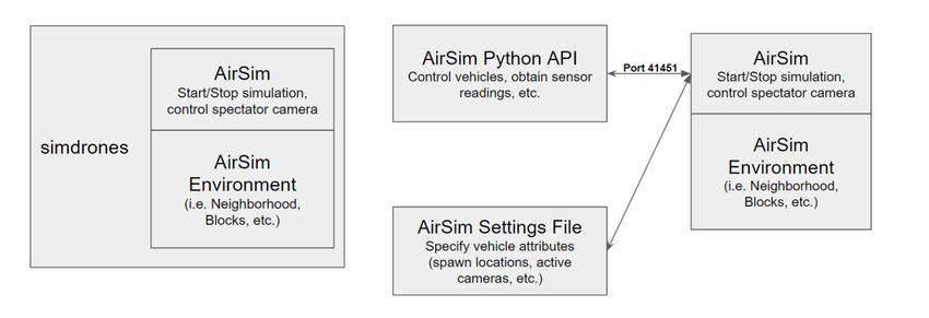
We benchmark the effects of communication modeling on this decentralized swarm task
through two metrics: convergence time and residual error (Figure 3.5) over 100 trials of each
configuration of communication model and agent count. Convergence time is defined as the
number of timesteps taken until all agents stop moving (i.e., until all agents individually
believe the line formation task has been achieved). Note that this captures only the local
belief state of the agents, and not the true global quality or convergence of the agent for-
mation into a line. Residual error, calculated directly from applying a standard line-fitting
least square procedure over the positions of all agents, shows the relative accuracy of a given
formation. Omitting details on the 6 different communication models employed, it becomes
clear from the benchmark results that communication has a large impact on the efficacy of
decentralized swarm systems (i.e. better communication results in less residual error and
faster convergence time), and thus the incorporation of communication into simulation and
swarm modeling is an essential consideration, especially in high-agent-count systems.CHAPTER 3. DEEP EMBEDDINGS FOR DECENTRALIZED SWARM SYSTEMS 23 Figure 3.4: Screen captures of swarm during line formation task under full communication at timesteps 0, 25, 50 respectively. Figure 3.5: Logarithmic least squares residual error (left) and timesteps to line formation convergence (right) of line formation task under varying number of agents and communica- tion models.
24

Chapter 4

Conclusions & Future Work

In this thesis, we have partitioned the problem of how best to counter pervasive intelli-
gent drone swarms using intelligent drone swarms into two areas: 1-vs-1 autonomous in-
terdiction, and N-vs-N decentralized swarm control; we also took a first step at examining
realistic communication models in this context. Through 1-vs-1 competitive self-play, we
observed emergent, complex maneuvering behaviours demonstrating reasoning about drone
capabilities, and continually improving drone dogfighting skills generation after generation.
In future work in this domain, it would be interesting to compare the performance of the
learned strategies against human drone pilots or manually designed, classical control meth-
ods (such as linear quadratic regulators); an additional venture would be to transfer the
learned policies to two physical drones (which AirSim is able to do directly), and demon-
strate the dogfighting drone trajectories with hardware. In N-vs-N perimeter defense, we
showed that homogeneous swarm reinforcement learning problems can benefit greatly from
carefully crafted state embeddings that leverage the advantageous properties of swarms by
respecting permutation and quantity invariances. In a problem setting where conventional
parameter-sharing proximal policy optimization fails to find an effective policy entirely, we
demonstrated that passing the state observations through adversarial mean embeddings or
adversarial attentional embeddings architecture allows the algorithm to produce effective,
decentralized swarm defense policies. An important next step in the future would be to
push the agent count up to perhaps thousands of agents, and then examine the relative
performance of various embedding techniques (and their performance in contrast to con-
catenation). Much like the case with 1-vs-1, demonstrating and evaluating these policies on
hardware would also prove to be a valuable future contribution by bridging the gap between
mere particle agents in simulation, and physical drones in reality.
You can also read