Mean circulation and EKE distribution in the Labrador Sea Water level of the subpolar North Atlantic
←
→
Page content transcription
If your browser does not render page correctly, please read the page content below
Ocean Sci., 14, 1167–1183, 2018
https://doi.org/10.5194/os-14-1167-2018
© Author(s) 2018. This work is distributed under
the Creative Commons Attribution 4.0 License.

Mean circulation and EKE distribution in the Labrador Sea Water
level of the subpolar North Atlantic
Jürgen Fischer, Johannes Karstensen, Marilena Oltmanns, and Sunke Schmidtko
GEOMAR Helmholtz Centre for Ocean Research Kiel, Düsternbrooker Weg 20, 24115 Kiel, Germany

Correspondence: Jürgen Fischer (jfischer@geomar.de) and Johannes Karstensen (jkarstensen@geomar.de)

Received: 26 April 2018 – Discussion started: 14 May 2018
Revised: 29 August 2018 – Accepted: 7 September 2018 – Published: 5 October 2018

Abstract. A long-term mean flow field for the subpolar           1   Introduction
North Atlantic region with a horizontal resolution of approx-
imately 25 km is created by gridding Argo-derived velocity       The subpolar North Atlantic (SPNA) has been in the focus
vectors using two different topography-following interpola-      of both observational and modeling efforts with regard to
tion schemes. The 10-day float displacements in the typi-        circulation- and water mass changes as part of the climate rel-
cal drift depths of 1000 to 1500 m represent the flow in the     evant Atlantic Meridional Overturning Circulation (AMOC;
Labrador Sea Water density range. Both mapping algorithms        e.g., reviewed by Daniault, et al., 2016). In this context the
separate the flow field into potential vorticity (PV) conserv-   intermediate depth circulation, which also determines the
ing, i.e., topography-following contribution and a deviating     spreading pathways of newly ventilated Labrador Sea Wa-
part, which we define as the eddy contribution. To verify the    ter (LSW) through the SPNA, is of specific importance and
significance of the separation, we compare the mean flow and     has been investigated from observations and models for sev-
the eddy kinetic energy (EKE), derived from both mapping         eral decades. A better understanding of the mechanisms that
algorithms, with those obtained from multiyear mooring ob-       control the transport properties at mid-ocean depth through
servations.                                                      the interplay of advection and diffusion is fundamental to our
   The PV-conserving mean flow is characterized by sta-          understanding of subpolar LSW circulation and export, and
ble boundary currents along all major topographic fea-           thus potentially subpolar AMOC contributions. Unlike the
tures including shelf breaks and basin-interior topographic      surface circulation, which can be analyzed for example from
ridges such as the Reykjanes Ridge or the Rockall Plateau.       satellite and drifter data, the intermediate depth circulation
Mid-basin northward advection pathways from the north-           and energetics is known to a much lesser extent. Studies that
eastern Labrador Sea into the Irminger Sea and from the          map energetics at the intermediate depth from observational
Mid-Atlantic Ridge region into the Iceland Basin are well-       data and at gyre scales are rare but identified, for example, as
resolved. An eastward flow is present across the southern        important evaluation metrics for basic verification of ocean
boundary of the subpolar gyre near 52◦ N, the latitude of the    model simulations, including the Coupled Model Intercom-
Charlie Gibbs Fracture Zone (CGFZ).                              parison Project (CMIP) models (Griffies et al., 2016).
   The mid-depth EKE field resembles most of the satellite-         In the late 1990s, the technology of profiling floats ad-
derived surface EKE field. However, noticeable differences       vanced such that investigations of the intermediate deep cir-
exist along the northward advection pathways in the Irminger     culation could be undertaken. Two experiments were car-
Sea and the Iceland Basin, where the deep EKE exceeds the        ried out in the western SPNA (mainly in the Labrador and
surface EKE field. Further, the ratio between mean flow and      Irminger seas) using Profiling ALACE (PALACE, where
the square root of the EKE, the Peclet number, reveals dis-      ALACE is the Autonomous Lagrangian Circulation Ex-
tinct advection-dominated regions as well as basin-interior      plorer) floats and are of special interest to the investigation
regimes in which mixing is prevailing.                           carried out herein. The first was by Lavender et al. (2000,
                                                                 2005) with a large fleet of floats drifting through the Labrador
                                                                 and Irminger seas at 700 m of depth (the approximate depth

Published by Copernicus Publications on behalf of the European Geosciences Union.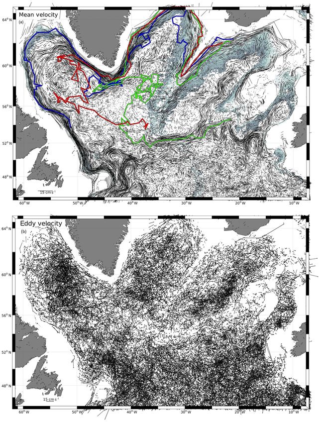
1168                            J. Fischer et al.: Mean circulation and EKE distribution in the Labrador Sea Water level

level of upper LSW in the SPNA). A major result of the study      vertical current shear is encountered. Thus, we will estimate
was that the intermediate depth circulation could well be de-     the advective part of the flow that is related to the concept of
scribed as a cyclonic boundary current system along the to-       potential vorticity (PV) conservation (LaCasce, 2000), and
pography and a series of anticyclonic recirculation cells ad-     the residual flow contribution that is attributed to the diffu-
jacent to the Deep Western Boundary Current (DWBC). The           sive part of the flow. Validation of this principle has been per-
second experiment was dedicated to the boundary current off       formed in the past (see Fischer and Schott, 2002; Fischer et
Labrador, and conducted in summers 1997 and 1999 with             al., 2004) through a comparison of deep displacements along
15 PALACE floats seeded into the DWBC off Labrador to             curved topography in relation to moored (Eulerian) records.
drift at 1500 m, the core depth of classical LSW (Fischer and         We focus here on the SPNA north of 45◦ N and make use
Schott, 2002). The main finding of this study, and contrary       of the extended set of Eulerian (current meter moorings) and
to the expectations, was that none of the floats were able to     Lagrangian (floats) observations available in the region. Over
exit the subpolar gyre via the boundary current route. Instead,   the previous two decades (regionally even longer) an impres-
some of the floats confirmed the existence of a recirculation     sive observing effort has been undertaken north of 45◦ N on
cell off Labrador and others indicated an eastward route fol-     the (intermediate) deep flow. Boundary currents are, thanks
lowing the North Atlantic Current (NAC) at its northeastern       to their strength, the prominent circulation features in the
pathway. This result stimulated a series of Lagrangian exper-     SPNA and found all along the shelf edges in particular on
iments (Bower et al., 2009) using RAFOS (where ROFAS              the western side of the gyre. However, there are also interior
is SOFAR spelled backwards with SOFAR meaning SOund               circulation features of both advective- and eddy-dominated
Fixing And Ranging) drifters but also model studies (e.g.,        patterns, and the primary research objective of this effort is to
Spall and Pickart, 2003).                                         discriminate the mean flow  from the turbulent (eddy)
   With the deployment of the global array of Argo profiling      component u0 of the flow field from which the deep EKE
floats at the end of the 1990s the number and spatial homo-       field could be determined.
geneity of displacement vectors at the floats parking depth           The paper is structured as follows. First, we briefly de-
of typically 1000 or 1500 m increased significantly. The data     scribe the methods to separate  and an accompanying
set is assembled in the YoMaHa’07 data base (Lebedev et al.,      u0 , obtained for each displacement vector from the differ-
2007). Based on this much larger database it is of interest to    ence between the observed displacement and the displace-
revisit the earlier results. One of the immediate questions is    ment projected to a PV contour. The fields obtained by two
how robust the earlier findings are; and moreover, whether        different gridding methods are verified for internal consis-
the present-day Argo data coverage would be sufficient to         tency, and in comparison to independent measurements from
prove and possibly refine the earlier results. There are two      mooring records. Next, a gridded velocity and an eddy ki-
approaches to these objectives: one is to investigate tempo-      netic energy (EKE) field of relatively high spatial resolution
ral changes in the deep circulation on interannual timescales     (on the order of 25 km grid size) for the SPNA is created by
but with a drawback on spatial resolution. Palter et al. (2016)   both gridding procedures. We discuss the fields for internal
followed that approach and found a slowdown in boundary           consistency based on major flow features. Furthermore, the
current flow in the Labrador Sea but no significant changes in    ratio of advective flow and diffusion (Peclet number) is es-
the large-scale subpolar gyre circulation. Another approach,      timated. The EKE field at depth is then compared with the
and this is taken here, is to neglect temporal variability and    EKE field at the surface, based on satellite data. The gridded
use all available displacement data for determining a mean        data sets are provided for download and further use, e.g., for
flow field on a finer spatial resolution that resembles narrow    model and data comparison; so far we are not aware of an
circulation elements in a higher resolution compared to what      intermediate depth EKE map.
has been discussed in the past.
   Several attempts have been undertaken to estimate advec-
tive (long-term mean) and diffusive contributions in the dis-     2   Material and methods
placement vectors on the basis of statistical and physical
constraints. While the displacements of the profiling floats      Two quality controlled Argo displacement (deep and surface)
may be well suited to determine the long-term mean of the         sets exist, but cover somewhat different time spans. Here, we
flow field, this is not straight forward for the eddy compo-      use the YoMaHa’07 Argo data set (Lebedev et al., 2007),
nent of the flow field (Davis, 2005; Davis et al., 2001). The     which contains estimates of velocities of deep and surface
author suggested calculating the diffusivity from displace-       currents using data of the trajectories from displacements be-
ment anomalies u0 calculated from the difference of the mean      tween consecutive dives of Argo floats. The YoMaHa’07 data
flow  and the measured displacement vector U m . Here,        set is frequently updated on a monthly basis.
we loosely follow the method proposed by Davis (1998),               This technical paper contains most of the necessary pro-
in which the mean flow is controlled by topography (f/H ,         cessing stages for both the deep and the surface velocity.
where H is the water depth), an assumption that should hold       There is also some discussion regarding the error sources
true in the SPNA regime where weak stratification and small       arising as a consequence of the 3-dimensional measure-

Ocean Sci., 14, 1167–1183, 2018                                                              www.ocean-sci.net/14/1167/2018/
J. Fischer et al.: Mean circulation and EKE distribution in the Labrador Sea Water level                                           1169

Figure 1. Data density in 1◦ × 1◦ fields; the number of 10-day displacement vectors per cell.

ments; in this report there is a discussion on the error as-            is discussed in Lebedev et al. (2007). The nominal position of
sessment of deep velocity due to vertical shear of horizontal           the velocity vector is the mean position between the descent
flow. While the floats are ascending from their drift, they will        and ascent position pair.
be subject to the flow field in the water column. In a weakly              The area under investigation ranges from 45◦ N, the lati-
sheared environment like the SPNA this effect is considered             tude just south of the Flemish Cap, to 65◦ N, which is just
to be small. However, there is a much larger error source               south of the Denmark Strait (Fig. 1). The westernmost longi-
that is due to calculating straight-line displacement vectors,          tude is 62◦ W, i.e., the Labrador shelf break, and to the east
which in the presence of curved bathymetry is large and has             the area is bounded at 7◦ W west of the British Isles. The evo-
a bias. This is illustrated by the following example of the             lution of the Argo data in this domain shows a rapid increase
DWBC surrounding Hamilton Bank near 55◦ N off Labrador.                 in data density in the first 5 years of the program (Fig. 2), and
A float that travels in this area at a mean speed of 15 cm s−1          from 2006 onwards the data density is adding around 2500 to
will pass around Hamilton Bank within one or two dive cy-               3000 displacement vectors per year; this is roughly equiva-
cles of the float. The difference between a straight-line dis-          lent to the number of temperature and salinity profiles gained
placement and the displacement estimated from the length                through Argo per year. Maximum annual data increase is
of, for example, the 1500 m isobath can be different by about           reached in 2011/2012 with 4000 additional current vectors
30 %; thus, the straight-line displacement is biased low espe-          each year. Thereafter, the yearly data gain stabilizes at 2500
cially in areas of high velocities and curved topography, e.g.,         to 3000 current vectors.
the DWBC.                                                                  The regional data density ranges from approximately 10 to
                                                                        more than 100 per bin (2◦ longitude × 1◦ latitude; Fig. 1); the
2.1   Temporal and spatial distribution of the Argo float               bin size corresponds with the typical area in which data will
      array                                                             be used for the interpolation to a certain grid point. Given the
                                                                        barotropic nature of the flow field in the SPNA, we merged
By March 2017 (this is the latest date considered for this              the displacement vectors from the two drift depths (1000
analysis) the displacement data set includes data from 4284             and 1500 m depths). Considering the temperature and salin-
floats stored in nine data assembly centers worldwide and               ity data recorded by the floats, the mean potential density
about 297 000 values of velocity. We define a velocity vector           field at 1500 m varies between σθ = 27.72 and 27.92 kg m−3
as the displacement between an Argo float descent (last sur-            with an average density of σθ = 27.77 kg m−3 . This density
face position) and the consecutive ascent (first surfacing po-          is slightly lower than the commonly used lower boundary of
sition) divided by the corresponding time difference. Some              classical LSW at σθ = 27.80 kg m−3 , and thus the resulting
inhomogeneity in position and time accuracy based on the                circulation pattern represents the core depth of the LSW.
communication and positioning technology (Argos, Iridium)

www.ocean-sci.net/14/1167/2018/                                                                     Ocean Sci., 14, 1167–1183, 2018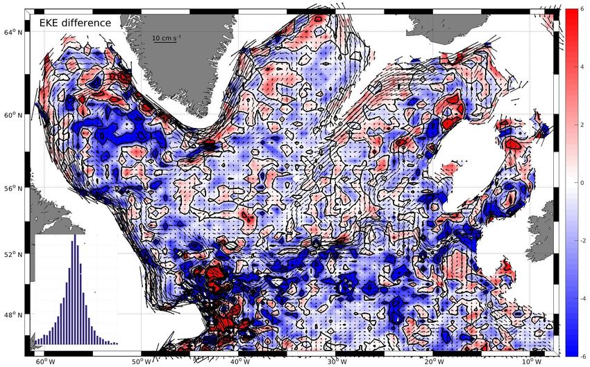
1170                              J. Fischer et al.: Mean circulation and EKE distribution in the Labrador Sea Water level

                                                                      procedure. Both methods use the same physical constraints,
                                                                      and both operate on an identical grid of 0.5◦ longitudinal
                                                                      range and 0.25◦ latitudinal range.

                                                                      2.3.1   Gaussian interpolation method

                                                                      The strategy of the GI method was to include two constraints
                                                                      in the interpolation procedure, namely a weighted distance
                                                                      between target (grid) point and data point, and the second
                                                                      is to reduce the influence of data points located in regions
                                                                      with very different water depths. The latter is a manifestation
                                                                      of our assumption that flow in the region follows PV con-
                                                                      tours. Thus, data points across the boundary current at steep
                                                                      topography would only weakly be influenced from nearby
                                                                      but much deeper or shallower locations outside the boundary
                                                                      current (a topography-following mapping).
                                                                         The weights used have a Gaussian shape described by
Figure 2. Temporal evolution of the Argo data density in the subpo-
lar domain independent of the parking depths (1000 and 1500 m),
                                                                      two parameters for each dimension: for the distance weight-
and from year 2000 to March 2017.                                     ing we chose 40 km for the half width of the Gaussian and
                                                                      80 km for the cut-off – such that points outside a radius of
                                                                      ∼ 80 km around a selected grid point will not be used. For
2.2    Auxiliary data                                                 the other dimension (water depth difference between data lo-
                                                                      cation and target location as a measure of PV difference), we
To estimate contours of constant PV defined as the Coriolis           chose 200 m half width and 600 m cut-off range. The choice
parameter divided by water depth (f/H ), we used the high-            of these values was guided by the dimensions of the bound-
resolution topographic data 2-minute Gridded Global Relief            ary current along steep topography (e.g., the Labrador shelf
Data (ETOPO2; National Geophysical Data Center, 2006).                break), with the width of the DWBC (Zantopp et al., 2017)
This topography is based on a combination of depth sound-             between 100 and 150 km, and a change of water depth across
ings and depth estimates from multiple sources and gridded            the DWBC from about 1000 to 3000 m. Through this proce-
to a 2 min special resolution. Only in one case we use the            dure, boundary currents would be conserved and not smeared
higher resolved ETOPO1 version, but this did not change the           out, while in the basin interior with a flat bottom the weight-
results.                                                              ing is more toward distance – with little influence of the un-
   Furthermore, we used altimetry-based absolute dynamic              derlying bathymetry.
topography from which the surface geostrophic flow and                   We analyzed the impact of different weights over a wide
EKE were derived (Le Traon et al., 1998). The altimeter               range of scales, but the selection applied here appears to gen-
products were produced by Ssalto/Duacs and distributed by             erate the most robust result with a clear definition of the
Aviso with support from CNES (http://www.aviso.altimetry.             circulation elements described hereafter. Using a higher re-
fr/duacs/). We used the gridded product with a 0.25◦ horizon-         solved grid (smaller scales) results in a noisier flow field with
tal resolution, similar to the resolution of the deep velocity        larger overall variance, while a coarser grid (together with
field. We note, however, that the surface EKE, derived from           larger interpolation scales) results in a smoother field and
this product, will be biased low as subgrid-scale variability is      certain details of the flow field are suppressed. The proce-
smoothed out.                                                         dure could be applied to both irregular target locations and
   Lastly, Eulerian time series data from moored instrumen-           regular grid locations.
tation that recorded in the depth interval considered in the             In a first processing step we separate the measurements
analysis here (1000–1500 m) were used to locally evaluate             into a mean flow contribution  and a fluctuating part u0
the results of the gridded data product (see Table 1 for an           that will be used later to determine the EKE field. Around
overview). Given the floats inherent sampling at 10 days, the         each measurement location we selected all data within the
moored records were smoothed accordingly.                             cut-off radius and by using the selected weights (see above)
                                                                      we estimate a mean flow vector at the measurement loca-
2.3    Separating mean flow and its fluctuation and                   tion by applying the above-described algorithm. Thus, we
       interpolation of the results                                   generate a velocity field that has the dimension of the orig-
                                                                      inal data set, and it contains only the weighted, PV-related
Two interpolation methods were used to map the displace-              ensemble-mean contribution (Fig. 3a). As an illustration, we
ment vector data: the first is a weighted Gaussian interpo-           show three floats that were deployed at roughly the same lo-
lation (GI) and the second is an optimum interpolation (OI)           cation in the northern Iceland Basin at water depths of around

Ocean Sci., 14, 1167–1183, 2018                                                                  www.ocean-sci.net/14/1167/2018/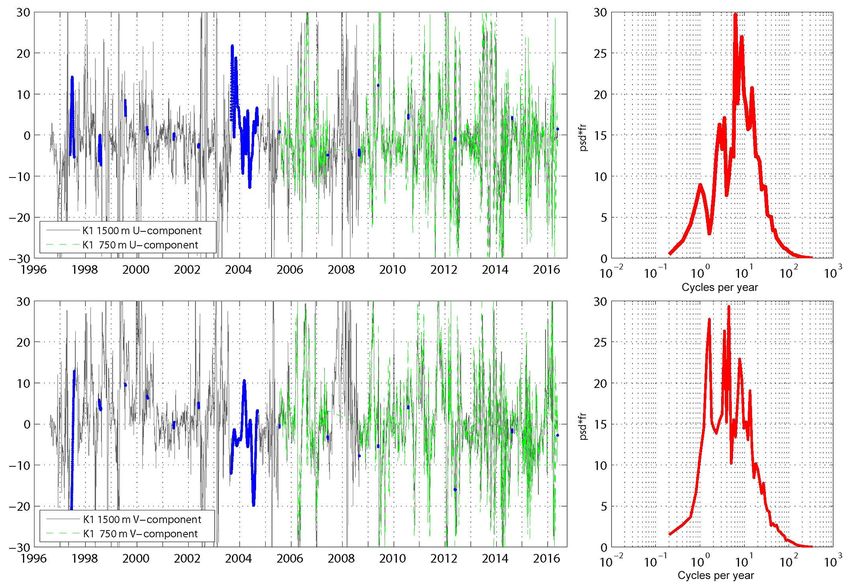
J. Fischer et al.: Mean circulation and EKE distribution in the Labrador Sea Water level 1171
Table 1. Eulerian EKE: statistics in the subpolar North Atlantic SPNA. BODC: British Oceanographic Data Centre (https://www.bodc.ac.uk/,
last access: March 2018).
Mooring nom- latitude longitude EKEFull EKE10dlp EKEGI Pe Comment
inal instrument cm s−1 cm2 s−2
depth cm2 s−2 2
cm s −2
Moorings in the northwest Atlantic
K421500 55◦ 27.50 N 53◦ 43.80 W 16.1 29 6 18 6.6 AR7W mooring
K491500 53◦ 08.50 N 50◦ 52.10 W 12.5 39 12 20 3.6 Records from the 53◦ N
K101500 53◦ 22.80 N 50◦ 15.60 W 0.2 13 7 13 0.1 observatory
K11500 56◦ 31.50 N 52◦ 39.00 W 1.6 165 72 34 0.2
Mid-basin moorings
CIS1000 59◦ 42.70 N 39◦ 36.20 W 1.6 37 21 20 0.3
OOI 59◦ 58.50 N 39◦ 28.90 W 1.9 63 25 20 0.4 OOI Irminger Sea (ac-
cess
K181500 46◦ 27.10 N 43◦ 25.10 W 4.3 78 50 52 0.6
Flemish Cap Moorings
B2271100 47◦ 06.20 N 43◦ 13.60 W 27.3 60 38 50 4.3
B11534 59◦ 48.50 N 32◦ 48.50 W 2.1 18 12 13 0.6 Reykjanes Ridge (ac-
cess via BODC)
KFA 59◦ 35.00 N 41◦ 33.00 W 18 9 12 Cape Farewell, NOCS
(access via BODC)
Moorings in the northeast Atlantic
I31135 62◦ 43.10 N 16◦ 49.20 W 6.1 110 26 16 1.2 Iceland array (access
I51403 62◦ 26.40 N 16◦ 28.30 W 3.1 90 54 21 0.4 via BODC)
S1245 61◦ 04.10 N 22◦ 11.50 W 4.5 47 17 16 1.1
O1480 60◦ 30.50 N 21◦ 36.10 W 4.0 68 39 24 0.6 ISOW transport array
W1520 59◦ 46.80 N 20◦ 56.60 W 1.0 133 90 48 0.1
J1 57◦ 12.90 N 10◦ 34.00 W 3.2 41 35 23 0.5 JASIN moorings (ac-
J2 57◦ 30.10 N 12◦ 16.00 W 3.3 44 37 22 0.5 cess via BODC)
C31290 54◦ 05.20 N 19◦ 55.00 W 5.6 15 8 17 2.0 Conslex moorings (ac-
C121260 53◦ 25.20 N 19◦ 18.00 W 2.8 35 27 23 0.5 cess via BODC)
E4 54◦ 24.80 N 25◦ 54.10 W 3.1 7 6 8 1.3 WOCE mooring
(access via BODC)
1800 to 2500 m. The length of the trajectories correspond separation of the measured displacement vectors into
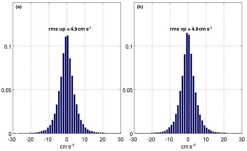
to more than 2 years elapsed since deployment. The floats (advective) and a fluctuating (eddy) component is success-
stayed within that depth range for a significant fraction of fully performed by the above methods, it allows one to calcu-
that time, and the close correspondence of the float trajecto- late u0 and v 0 , the fluctuating (eddy) velocity contribution of
ries and the shaded area is an indication of the PV-following each displacement vector (Fig. 3b). Both eddy components
nature of the deep flow field. show similar overall (basin wide) statistics of a Gaussian
Subsequently we applied the mapping procedure to the shape and equal rms values of 4.9 cm s−1 (Fig. 4). The sec-
measured velocity field (Um ) to obtain a field on a regular ond final data product is the gridded EKE produced from the
0.5◦ longitude × 0.25◦ latitudinal grid and the result is u0 and v 0 fields derived through the first interpolation step.
on a regular grid, which is considered as one of our final data
products. 2.3.2 Optimum interpolation method
After estimating the mean velocity from the displacement
vectors, we calculated the residual flow components (u0 and The second procedure uses the method of optimum interpo-
v 0 ) by subtracting the mean component from the original data lation (OI method), similar to the one described in detail in
(Fig. 3b). The EKE is estimated independently for each of the Schmidtko et al. (2013). Data were only mapped if the grid
two interpolation methods (GI and OI). Assuming that the points have a water depth deeper than 1200 m according to
www.ocean-sci.net/14/1167/2018/ Ocean Sci., 14, 1167–1183, 2018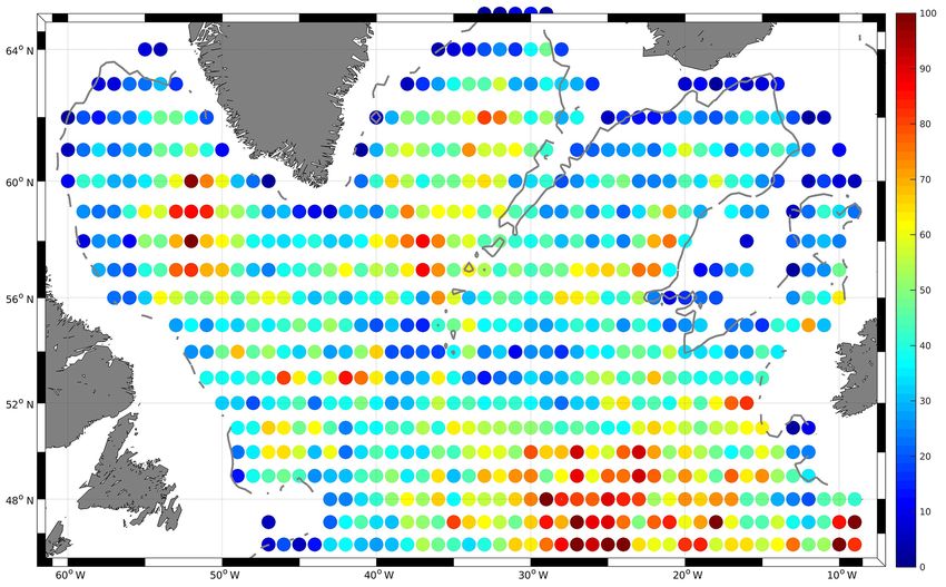
1172                               J. Fischer et al.: Mean circulation and EKE distribution in the Labrador Sea Water level

Figure 3. Mid-depth circulation (a) in the western SPNA from ∼ 38 500 Argo deep drifts (1000 or 1500 m parking depth) derived from
the YoMaHa’07 data. This is an attempt to present the advective contribution of the flow field at each measurement location; i.e., for each
measured 10-day drift vector (for details of the processing see text). Colored lines for selected float trajectories (deployed in the Iceland
Basin); blue shaded area is for the topographic depth range (1500 to 2500 m). The residual (b) is thought to be u0 , the eddy velocity
contribution to the flow field.

the topographic data set. All data within a radius of 110 km                The field, resulting from the OI was used as the mean
and at locations with similar water depths – less than 1000 m            flow field , which was then used to compute the resid-
difference – were used in the OI. Linear gradients in latitu-            ual flow (u0 ) from each displacement vector (Um ) by lin-
dinal direction, longitudinal direction, and water depth were            ear four-point interpolation. An individual EKE value was
fitted to the data. For the covariance matrix a diagonal value           computed for each displacement. To exclude extreme out-
of 1.5 was used as an estimate for the signal-to-noise ra-               liers, an interquartile range filter was applied, rejecting data
tio (see Schmidtko et al., 2013 for details). The background             points 2.2 times the interquartile range above the third quar-
field used in the OI was taken from a least squares linear and           tile or that range below the first quartile. This is similar to
quadratic fit of the data using depth, longitude, and latitude.          a 99.98 % standard deviation filter in the case of normal dis-

Ocean Sci., 14, 1167–1183, 2018                                                                       www.ocean-sci.net/14/1167/2018/
J. Fischer et al.: Mean circulation and EKE distribution in the Labrador Sea Water level                                          1173

Figure 4. Normalized distribution of the mid-depth eddy velocity components; (a) is u0 (east–west component) and (b) is v 0 (north–south
component) – Gaussian distribution with equal rms of 4.9 cm s−1 .

tributed data. The EKE data were then mapped in an identical          take a northward drift on the western side of RR in the
procedure as the mean field.                                          boundary current that surrounds the northern Irminger Sea
                                                                      and downstream merge into the deep East Greenland Current
                                                                      (dEGC). The selected floats stayed for almost 2 years in the
3     Results                                                         deep boundary current inshore of the 1800 m isobaths before
                                                                      they reached Cape Farewell, the southern tip of Greenland
3.1     The intermediate depth large-scale circulation                and which is about 2500 km downstream (comparable with a
        from a displacement vector point of view                      mean drift speed of about 4 cm s−1 ). At about the latitude of
                                                                      Cape Farewell, the northward flow along the western flank
First we inspected the GI-based interpolation of  on              of the RR is on the order of 5 cm s−1 , while the southward
the original displacement vector positions, which represents          flow along the east Greenland shelf break regionally exceeds
individual mean flow realizations and added a number of se-           10 cm s−1 . The trajectories clearly show that the PV (depth)
lected float trajectories (Fig. 3a). The flow realizations nicely     constraint on the flow is very strong and as such our gridding
sample the different flow regimes in the SPNA and cover               procedure appropriate.
the boundary currents; flow associated with topographic fea-
tures, such as the Mid-Atlantic Ridge; and prominent flow             3.1.2   Labrador Sea
features, such as the deep extension of the NAC in the NWC.
Selected areas are discussed in the following sections.               The intermediate circulation in the Labrador See shows nar-
                                                                      row cyclonic boundary circulation where the topography is
3.1.1    Boundary currents                                            steep, i.e., along the East Greenland and Labrador shelf
                                                                      breaks (Fig. 3a), while in regions with a gentler slope (e.g.,
Individual mean flow realizations sample the boundary cur-            northern part of the Labrador Sea) the boundary current
rents and indicate the coherence of the flow along the to-            widens considerably. From the boundary current to the in-
pography. This is also confirmed by individual float trajec-          terior Labrador Sea the flow reveals stable but weak re-
tories. Individual floats that were released in the northern          circulation cells with cyclonic rotation, and the interior of
Iceland Basin, near the northernmost part of the Reykjanes            these elongated cells is almost stagnant, as is also seen in
Ridge (RR), follow the deep boundary current along the to-            time series measurements (Fischer et al., 2010) of the 53◦
pographic slope of the RR southwestward. The displacement             moored array at location K10, where the mean 1500 m flow
vectors indicate swift speeds of approximately 6 to 7 cm s−1 .        is 0.8 cm s−1 northwestward, and at K9 where the mean flow
For the selected floats, it takes about 3 months to reach the         is 12.5 cm s−1 but southeastward (Fig. 5b; Table 1).
first gaps in the RR and thus to enter the Irminger Basin.               The nearly stagnant, weakly anticyclonic circulation is ob-
However, different gaps exist and influence the exchange              served for the area where deep convection takes place. Here
with the Irminger Basin. After crossing the RR, the floats            the water is trapped within the closed circulation in the re-

www.ocean-sci.net/14/1167/2018/                                                                    Ocean Sci., 14, 1167–1183, 2018
1174 J. Fischer et al.: Mean circulation and EKE distribution in the Labrador Sea Water level
gion of strong wintertime buoyancy loss. Both the cyclonic ing at the topography (still at the latitude of the CGFZ, i.e.,
recirculation cells along the Labrador shelf break and the 52◦ N). Thereafter, the flow follows the topography north-
anticyclonic interior are thus favorable for deep convection. ward into the Rockall Trough west of Ireland. On the western
At 1500 m depth, the lightest water is found in the central flank of the Rockall Plateau, a narrow eastern boundary cur-
Labrador Sea and is surrounded by extremely weak (on the rent forms and flows northward until it reaches the Iceland–
order of 1 cm s−1 ) anticyclonic flow. Eventually the water Scotland Ridge, where it feeds the southwestward boundary
in the central Labrador Sea feeds the advective path around current (discussed above) that eventually becomes a “west-
Cape Farewell thereby exporting light and weakly stratified ern” boundary current along the RR. However, the broadest
water into the Irminger Sea. Further south, at the exit of the inflow comes from the mid-basin flow regime that extends
Labrador Sea, the flow enters a very active eddy regime in from the NAC northward from about 27◦ W, and follows the
a region with very variable topography – the Orphan Knoll deep trench northward to 62◦ N. This mid-basin flow is char-
region near 47◦ W, 51◦ N. Here the northwest corner of the acterized by stable advection and several large wave number
NAC and the outflow of the Labrador Sea merge and inter- meanders.
act.
3.1.5 The North Atlantic Current regime
3.1.3 Irminger Sea
The southern exit of the Labrador Sea is the region where
The Irminger Sea has several characteristic flow patterns at the NAC meets the DWBC (Fig. 5a); and while the LSW
intermediate depth (Fig. 3a). The most pronounced feature is follows the topography inside a topographic feature called
the dEGC that exists over the whole western part of the basin. “Orphan Knoll” (50◦ N, 46◦ W), the NAC is located seaward
On the opposite side the Irminger Sea is bounded by the RR of the Orphan Knoll and is retroflected toward the east in a
that is a barrier for most of the flow beneath 1000 m depth. feature known as the NWC. The latitude of the NWC is also
Further south, several gaps in the ridge allow the water from at 52◦ N, and from there the NAC meanders eastward through
the eastern basin to spill over the ridge and a northward deep the CGFZ. The zonal flow field and the associated southern
boundary current forms along the western flank of the ridge. signature of the polar front can be interpreted as the southern
This is one source of the dEGC. A second source of the inter- limit of the SPNA and it forms the zonal component of the
mediate dEGC is the mid-basin current band that is fed from large-scale cyclonic circulation. In the LSW depth range the
the Labrador Sea and extends up to 64◦ N where it enters the Polar-Front separates the lighter water to the south from the
dEGC; the cyclonic circulation that this mid-basin vein forms denser subpolar gyre.
is sometimes called the Irminger Gyre. Within the Irminger
Gyre, a number of long-term moorings have been maintained 3.2 Gridded mean flow
for more than a decade to record the thermohaline evolution
of the gyre center and possibly deep convection underneath By application of the GI method, the velocity field was in-
the Greenland tip jet (e.g., Pickart et al., 2003); the moor- terpolated to a regular grid of 0.25◦ latitude and 0.5◦ longi-
ings are nowadays incorporated into the international OS- tude (Fig. 5a). As for the raw data maps (Fig. 3a) the gridded
NAP (Overturning in the Subpolar North Atlantic Program) data reflect all the major circulation elements. The interpo-
program (Lozier et al., 2016) and the OOI (Ocean Observa- lation method keeps the deep boundary currents as narrow
tories Initiative, http://ooinet.oceanobservatories.org, last ac- and stable jets that are resolved by five or more grid points.
cess: March 2018). The mid-basin current band appears to Mid-basin jets in the Irminger Sea and the Iceland Basin ap-
have a number of meanders that are also visible in the 1500 m pear as continuous but meandering pathways of the inter-
geopotential derived from the Argo profile data. mediate deep circulation. The correspondence of the current
field and the potential density at 1500 m depth is evident. The
3.1.4 Iceland Basin strongest density gradients are associated with the western
boundary current elements along the eastern RR, associated
The Iceland Basin, which is less well investigated, has two with the East Greenland Current (EGC), and to a lesser ex-
major topographic features that influence the circulation tent with the Deep Labrador Current. In combination with
strongly. The western limit of the Iceland Basin is the RR the deep density, the major export routes for newly venti-
that shows the already discussed boundary current. At the lo- lated LSW are also visible in the potential density pool of the
cation of the CGFZ, which is at about 52◦ N, dynamically central Labrador Sea draining into the Irminger Sea. There
forms the southern boundary of the basin and where the cir- is also a connection between the NWC and the convection
culation at the LSW depth is eastward in connection to the area by a low density anomaly that is not associated with the
NAC supplying water towards the eastern SPNA. DWBC, but with the reverse circulation into the Labrador
Two branches of the NAC are evident (Fig. 3a): the ma- Sea.
jority of the floats drift far eastward in a strongly mean- Although, we only show the mean gridded flow field from
dering current band (300–350 km wavelength) until arriv- the GI method we do obtain the same results from the OI
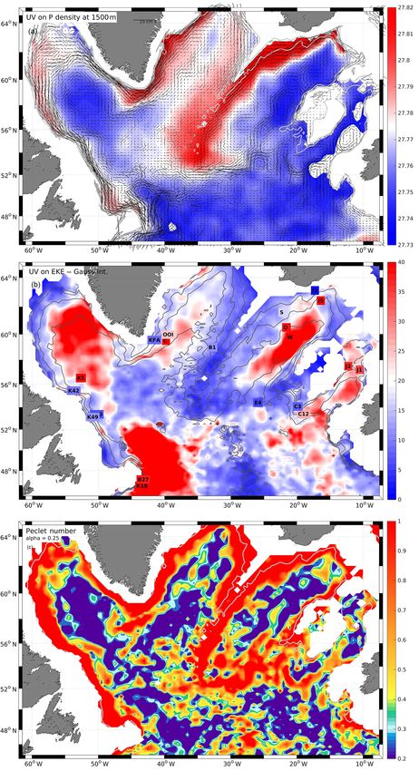
Ocean Sci., 14, 1167–1183, 2018 www.ocean-sci.net/14/1167/2018/J. Fischer et al.: Mean circulation and EKE distribution in the Labrador Sea Water level 1175 Figure 5. (a) Gridded velocity field from the GI method overlaid on potential density distribution from 1500 m depth. (b) Gridded EKE (in cm2 s−2 ) map from the GI method with selected EKE values from moored observations (numbers in boxes). Mooring fluctuations are low- pass filtered at 10 days cut-off for better comparability of mooring time series with 10-day displacement velocity from Argo data. Mooring location markers are colored with respect to the EKE from the moored record; color map is identical to that of the background field. (c) The ratio of mean speed to the square root of the EKE scaled by a factor alpha = 0.25, i.e., a measure of the Peclet number P e. www.ocean-sci.net/14/1167/2018/ Ocean Sci., 14, 1167–1183, 2018
1176                               J. Fischer et al.: Mean circulation and EKE distribution in the Labrador Sea Water level

method. The differences in the two estimations mainly con-         slope. This is further supported by the weak EKE in the
tain small-scale elements that reflect the scales of the influ-    southward flowing East Greenland Current.
encing radii by either method.
                                                                   3.4     Advection versus diffusion – Peclet number
3.3    Gridded eddy kinetic energy
                                                                   The western subpolar basin has very different regimes re-
From the individual u0   and v 0fields we generated a smoothed     garding mean flow and EKE pattern. Even at greater depths,
and gridded version of the EKE (Fig. 5b) using the same in-        there are narrow boundary currents along the topography, in-
terpolation parameters as for the mean field – i.e., both fields   terior persistent current bands, and regimes of almost stag-
have the same length scales in consideration, and the grid         nant mean flow with intense eddy motion, but it is a priori not
is identical. “Smoothed” also means that some de-spiking           clear which of the processes – advection or diffusion – dom-
and noise reduction during the gridding operation was ap-          inates in either of the circulation regimes. This objective is
plied, as there were a few individual spikes along the edges       investigated through the calculation of a local dimensionless
of the mapping environment, i.e., in regions where the map-        number, the Peclet Number (P e), which is the ratio of advec-
ping area intersects the 1500 m topography and where floats        tion to diffusion. Here, we calculate a simplistic P e version
might have become bottom-stuck. These spikes could be eas-         that allows one to regionally compare the relative importance
ily detected and accounted to less than 2 % of the data con-       of advection versus diffusion:
tributing to an individual grid point. As a result the cleaned                                  √
EKE distribution is smoother and more reliable.                    P e = Ld · /K, with K = α EKE · Ld ;                   (1)
   We note several intense EKE hot spots in the Labrador                 for EKE see Figs. 3b, 6a;
Sea, in the NWC of the NAC, and in the eastern SPNA lo-
cated east and west of the Rockall Plateau. While it is not        α is an empirical (non physical) scaling factor; here we chose
surprising that the retroflection of the NAC (i.e., the NWC)       α = 0.25, such that the resulting P e field varies between 0
shows large EKE values exceeding 250 cm2 s−2 , it is sur-          and 1; Ld is the Lagrangian length scale chosen to be related
prising that the zonal basin-crossing of the NAC has rela-         to the first baroclinic Rossby radius (on the order of 1 to 2 ×
tively weak EKE at LSW levels. The second strongest EKE            104 m) (see Chelton et al., 1998);  is the mean current
is located in the northeastern Labrador Sea and is generated       speed taken from the gridded velocity fields.
by instabilities and eddy shedding of the West Greenland              The resulting P e distribution (Fig. 5c) basically shows two
Current (WGC), known to occur from surface flow obser-             regimes; one with very small P e (i.e., P e
J. Fischer et al.: Mean circulation and EKE distribution in the Labrador Sea Water level 1177
Figure 6. EKE map difference between optimum interpolation (OI) and Gaussian interpolation methods. Inset at lower left: histogram of
difference reveals Gaussian shape and a weak bias of = −1 cm2 s−2 .
4 Verifications of the results note that each of the mapping procedures requires de-spiking
of the velocities (e.g., see spikes in the eddy field near the
We verified our results in three different ways. First the boundary, Fig. 3), which is treated differently in the two
results from GI and OI were compared in order to iden- methods. The strongest impact on the EKE field is due to the
tify a superior interpolation method. Then we compared the removal of individual large velocity spikes in the GI method,
mean flow and mean EKE fields with similar quantities de- which leads to a regional reduction of the corresponding
rived from Eulerian time series data from moored stations EKE field. In this procedure we sorted the selected eddy ve-
(EKEmoor ) in the region; and the third way of verification locity data (typically within the cut-off scales, on the order
was a comparison between the deep EKE and the EKEsurf of 100 km, about 100–200 data points) with respect to their
from satellite sea-level anomaly (SLA) data. magnitude, and removed the largest of the data. Removing
only the largest 1 % of eddy velocities results in a positive
4.1 Consistency of interpolation techniques bias of 4 cm2 s−2 . When using additional statistical criteria,
e.g., removal of data only if exceeding a threshold based on
The mean flow fields from the two gridding methods are
statistics (like 2 times the standard deviation), then the bias
surprisingly similar and there are no significant differences
would be in the range 1 to 2 cm2 s−2 . This might be taken as
between the velocity and speed fields. The overall speed-
a cautionary hint for interpreting the EKE map as a quantita-
difference is −0.16 cm s−1 , which illustrates that there are
tive measure for the small-scale details of the eddy field. No
no systematic differences (biases) between the two speed es-
explicit de-spiking has to be used in the OI method, as it is
timates as a result of the gridding technique. The difference
inherent in the method itself (see Schmidtko et al., 2013).
field is patchy in structure with patch scales on the order of
the interpolation radii. Thus, by choosing the GI method, the 4.2 Comparison with local Eulerian measurements
current map (Fig. 5a) is considered to be representative and
independent of the two mapping procedures applied. The second method for verification was a comparison be-
Likewise, the difference in GI and OI EKE fields (Fig. 6) tween the derived mean fields ( and EKE) and selected
agreed well. Most of the EKE differences occurred in the locations where time series data from moored instrumenta-
range ±5 cm2 s−2 with the strongest deviations around the tion was available (Fig. 5b; Table 1).
NAC path across the SPNA; here, the GI method produces
somewhat larger values. In contrast, the NWC reveals larger 4.2.1 Labrador and Irminger seas
EKE values for the OI method. A patchy structure is ob-
served with scales associated to the influencing radii of In the convection area of the Labrador Sea, a time series
the gridding methods (roughly 100 km). The difference has of currents is available at the K1 site since 1996 (the site
an overall Gaussian distribution but with a slight bias of is close to where the Ocean Weather Ship Bravo; 56◦ 300 N,
1 cm2 s−2 toward larger EKE in the OI method map. We 51◦ 000 W; was operated; Fig. 7). In general the mean flow at
www.ocean-sci.net/14/1167/2018/ Ocean Sci., 14, 1167–1183, 20181178 J. Fischer et al.: Mean circulation and EKE distribution in the Labrador Sea Water level Figure 7. Example of a current time series from the central Labrador Sea at mooring K1. Two depth levels were occupied regularly (750 m since 2006, green curve; 1500 m since 1996). Gaps (blue lines) are filled by interpolation based on empirical orthogonal functions (Zantopp et al., 2017). High-frequency spectra from 1500 m records (right column). the location of K1 is very weak (on the order of 1 cm s−1 ) In the boundary current system of the Labrador Sea a with a northwestward direction into the Labrador Sea and, number of records could be analyzed. In general, the flow given the mooring position, consistent with the anticyclonic is rather stable and strong (Lazier and Wright, 1993; Fis- circulation around the basin center (Fig. 5a). Short timescales cher et al., 2004; see also Table 1). Representative for the dominate the variability in the flow (Fig. 7), and the spec- DWBC at 53◦ N (K9, Zantopp et al., 2017), the long-term tra indicate that the bulk of the energy is on intra-seasonal mean flow along the topography is 12.5 cm s−1 and the EKE periods with strong decay toward longer timescales. The (again for periods less than 180 days) is 62 cm2 s−2 . Farther strongest variations occur in late spring and are associated toward the topography, the mean speed is even larger and the with eddies shed by the WGC near the location of Cape Des- EKE smaller, as the DWBC appears to be more focused by olation (Avsic et al., 2006; Funk et al., 2009). These eddies the steep topography at 53◦ N. In any of the boundary cur- are only weakly sheared in the LSW depth range which is an rent records a large energy contribution is on timescales less important aspect as it supports combining 1000 and 1500 m than 10 to 20 days (Fischer et al., 2015), which are not cap- parking depths for Argo float displacements. The EKE from tured by the Argo displacement vectors and different from 180-day high-pass filtered time series is around 170 cm2 s−2 the basin interior were the flow variability is on timescales in both levels (750 and 1500 m; Table 1). These values are longer than a month and thus better resolved by 10-day dis- larger than what is derived from the Argo data set and we in- placement vectors from Argo (Fig. 8). terpret this to be a result of the inherent low-pass filter in the In the records in the center of the DWBC at Hamilton float processing. With respect to the P e (Fig. 5c), the area is Bank, the total EKE of the moored record is larger than that characterized as an eddy-dominated regime. from the float displacement but similar to K9 (Table 1). For a In the CIS a current time series is available at about better comparison we calculated the EKE fraction that Argo 1000 m depth. As for K1, the site is characterized by a weak would represent in their 10-day displacement vectors by low- mean flow (around 1 cm s−1 ), while the EKE (based on intra- pass filtering the mooring data (10 days cut-off period of seasonal velocity fluctuations) is around 80 cm2 s−2 (Fan et the filter). Then, the EKE values coincide much better as is al., 2013). The location of CIS is at the edge of the mid-basin demonstrated by the colored mooring numbers in Fig. 5b. velocity band connecting the Labrador Sea around the tip of Near the offshore edge of the DWBC, at mooring K10 of Greenland, and into the Irminger Sea. the 53◦ N array, the flow speed is rather low, as the moor- Ocean Sci., 14, 1167–1183, 2018 www.ocean-sci.net/14/1167/2018/
J. Fischer et al.: Mean circulation and EKE distribution in the Labrador Sea Water level                                             1179

Figure 8. (a) Surface EKE derived from the AVISO geostrophic surface flow that is high-pass filtered at 180-day cut-off (in cm2 s−2 ) as an
estimate of the geostrophic turbulence. Overlaid is the Argo-derived mean (PV-related) flow at 1000–1500 m depth, with flow speeds below
1.5 cm s−1 omitted; this better reveals the major advective pathways. (b) The logarithmic ratio of surface EKE to deep EKE; green and blue
colors show areas in which the deep EKE dominates.

ing lies in the transition regime between the DWBC and the              from the mean current map and the density field it is tempt-
recirculation pathway in the upper 2000 m; while at deeper              ing to assume this route as one of the supply routes for the
depths it is still part of the DWBC (Zantopp et al., 2017). At          deep central Labrador Sea.
1500 m the flow is mainly the reverse of the DWBC direction
and the EKE is rather small, but in good agreement with the             4.2.2   Subpolar locations
EKE from Argo.
   Associated with weak mean speeds (only 10 % of the                   Moored observations in the Iceland Scotland Overflow Wa-
DWBC speed is found at locations offshore of K10) and                   ter were available at four positions (Named I, S, O, and W;
moderate EKEmoor , values coincide when the resulting Peclet            see Kanzow and Zenk, 2014). Only three (S, O, W) moorings
numbers (Fig. 5c; Table 1) are low and indicate sufficient dif-         delivered data in the appropriate depth range for this study.
fusion in the presence of weak advection. This structure is re-         While S was located in the area of low deep EKE, the fluc-
flected in the Argo flow pattern, which shows an increasing             tuations increase toward east with mooring W located in the
advective contribution further toward the basin interior, and           EKE max along the northward flow (Fig. 5a).

www.ocean-sci.net/14/1167/2018/                                                                      Ocean Sci., 14, 1167–1183, 2018
1180 J. Fischer et al.: Mean circulation and EKE distribution in the Labrador Sea Water level
North of the I S O W array the Iceland array is located at with less slope, i.e., the northern Labrador Sea we observe
the shelf break south of Iceland, and the northern mooring di- strong EKE at all levels (surface and LSW depth range). This
rect at the topography reflects the low EKEmoor typical for to- is the area where the deep WGC turns away from the steep
pographically guided currents, while the one further offshore Greenlandic shelf and intense eddies are formed and shed
is located in the northern extension of the EKE maximum of from the DWBC (Eden and Böning, 2002).
the Iceland Basin. Following Ollitraut and de Verdiere (2013) we calculated
During the JASIN program in the late 1970s a number the logarithmic ratio of surface EKE to the deep EKE; i.e.,
of moorings were deployed in the northern Rockall Trough ln(EKEsurf /EKE), such that the ratio becomes negative when
(Gould et al., 1982) and these moorings reflect the interme- the deep EKE is larger than that at the surface. Generally,
diate intensity of the deep EKEmoor that is also present in the in a baroclinic ocean one would expect positive ratios, with
Argo-derived values (Table 1). the EKEsurf sufficiently larger than the EKE at depth, as is
The EKE from the moorings represent mean regional vari- the case for the region south of the North Atlantic Drift, i.e.,
ations. In order to compare the high-resolution time series south of 52◦ N. A global much coarser map of such a ratio re-
with the Argo data, a 10-day low-pass filter is applied. There veals that this is the case for almost the whole Atlantic Ocean
is a remaining discrepancy between EKE from Argo and (Ollitraut and de Verdiere, 2013). In their paper, the SPNA
from moorings with a tendency that in regions with low EKE appears as broad negative area in which the deep EKE ex-
(taking now the Argo-derived map as a reference) the Argo ceeds the upper layer or is of similar magnitude. The much
estimates are larger than the 10-day low-pass filtered moor- higher resolution of the field generated herein (Fig. 8b) al-
ing estimates, while in regions of high EKE the situation is lows for a more detailed view, which reveals two centers of
reversed. We interpret this discrepancy by the inherent (non- deep EKE dominance. The first is associated with the DWBC
linear) temporal filtering in the EKE derived from Argo that all along the Labrador shelf break and the strongest signal
tend to low-pass filter the field with unpredictable filter char- around Hamilton Bank. The second center is associated with
acteristics (depending at which times the floats enter the cor- the deep action center south of Cape Farewell that shows both
responding interpolation radius). stable advection and EKE at depth, while at the surface these
components are rather weak. This zone extends far north
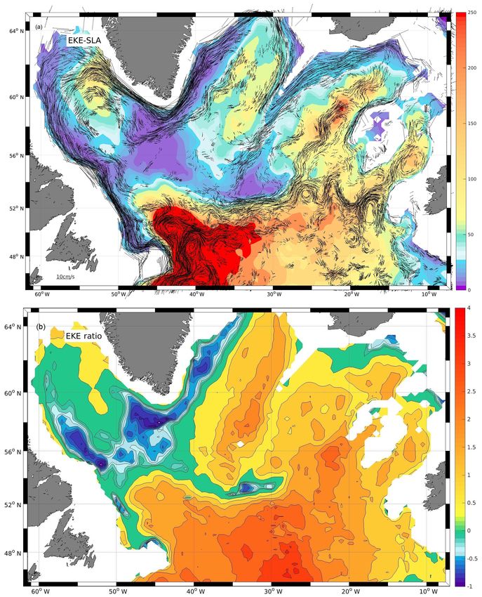
4.3 Surface EKE versus intermediate depth EKE into the Irminger Sea where it appears to be related to the
deep EGC and its variability. This behavior indicates that for
In addition to the deep EKE we estimated the surface EKE the inter-basin spreading and mixing of newly formed water
(EKEsurf ) field calculated from remote sensing-based abso- masses the deep EKE field contains important information ,
lute dynamic topography observations. The geostrophic sur- which is not easily available elsewhere; at least not from the
face flow from SLA contains variability over a wide range surface variability alone.
of frequencies, and some of the long-term components are Besides the boundary-current-related anomalies there is
not generally thought to be part of the turbulent eddy field. one additional zone in which the deep EKE is close to the
Thus, we extracted the intra-seasonal variability by apply- surface EKE, and that is along the CGFZ at the northern flank
ing a high-pass filter (Hanning window) with a cut-off period of the NAC. In this area the flow is guided by the deep topog-
at 180 days. The result is a field of geostrophic fluctuations raphy and advection appears to be dominating the zonal flow
from which we calculate EKEsurf (Fig. 8a). This field is inde- (relatively large P e).
pendently derived, and thus allows for an independent com-
parison of the Argo-derived fields (here, the deep circulation
and EKE). 5 Summary and conclusion
The EKEsurf also resembles major (deep) circulation ele-
The results of the investigation can be summarized as fol-
ments, such that the zonal flow in the CGFZ region located
lows:
underneath the zone of maximum EKEsurf gradient at the sur-
face. (Note in Fig. 8 only currents larger than 1.5 cm s−1 are 1. Based on nearly 17 years of quality controlled Argo
shown, and thus only vector magnitudes that would be suffi- displacement vectors, a high-resolution (∼ 25 km grid)
cient to travel one Rossby radius within the 10-day schedule map of mean flow in the depth layer of the LSW was
of the floats are included). A similar surface versus deep EKE constructed for the subpolar North Atlantic (SPNA).
and flow pattern is seen for the northeastern flow from the Robust circulation elements were identified consisting
Labrador Sea into the Irminger Sea. Within the Iceland Basin of boundary currents along topographic slopes, mid-
the deep flow is associated with the surface EKEsurf maxi- basin advective pathways, and stagnation regimes with
mum, suggesting the mid-basin path is present from surface very low mean speeds.
to LSW depth range. Interestingly, the surface EKE shows
a clear EKE minimum all along the DWBC in the western 2. The mapping procedures were twofold: Gaussian in-
SPNA, and this is due to the slanting shape of the boundary terpolation (GI) and optimum interpolation (OI), both
circulation and the slope of the western shelves. In a region methods were applied using potential vorticity (PV)
Ocean Sci., 14, 1167–1183, 2018 www.ocean-sci.net/14/1167/2018/J. Fischer et al.: Mean circulation and EKE distribution in the Labrador Sea Water level 1181
constraints, and the resulting mean flow fields were very (e.g., Straneo et al., 2003) in which the export of LSW into
similar – almost identical. the Irminger Sea, and the boundary current export around the
Flemish Cap were identified as major export routes. While
3. The second product was the fluctuating (eddy – u0 , v 0 ) the Irminger Sea route appears strong and robust, the flow
velocity component, which was determined as the resid- along the topography (Flemish Cap) is relatively narrow and
ual after subtracting the average and PV-conserving the EKE maximum in this region is due to the NAC interac-
contribution from the individual measurements (dis- tion with the upper part of the DWBC near the steep topo-
placement vectors). The u0 , v 0 fields were used to map graphic slope. Another major export route is into the eastern
the mean EKE distribution, to our knowledge for the SPNA via the NAC path along 52◦ N.
first time. Traditionally the upper ocean eddy variability represented
4. The ratio of mapped mean flow to the square root of by the EKE distribution has been investigated from SLA data
the EKE, the Peclet number (P e), was estimated and (Brandt et al., 2004; Funk et al., 2009). Just recently (Zhang
showed regions that are advection dominated (boundary and Yan, 2018), the Labrador Sea surface EKE based on al-
currents and internal LSW routes), and regions with low timeter data has been investigated with regard to interannual
PE, in which eddy diffusion prevails. to decadal variability in the time period 1993 to 2012. They
find strong interannual variability in the EKE field near the
5. The mapped fields were analyzed for consistency be- WGC, but no trend over the observational period.
tween the OI and GI methods. In addition velocity time Generally, mid-depth EKE maps based on observational
series from moored sensors were used to estimate mean data are rare but important for the deep ocean water mass and
flow and EKE in an attempt to verify the mapped fields tracer spreading. Thus, both the mean current field and the
locally with independent data. While the general pat- EKE at the transition between the deep water masses LSW
tern of high and low EKE regimes are consistent, the to LNADW should be useful metrics for ocean model evalu-
mooring EKE appears to be larger than EKE from Argo, ations.
but the differences become smaller when the Eulerian
measurements are low-pass filtered with a cut-off at the
Argo sampling timescale (10 days). Data availability. The raw open-access data are available from the
YoMaHa’07 (http://apdrc.soest.hawaii.edu/projects/yomaha/index.
6. Comparing the mid-depth EKE with the independently php, Lebedev et al., 2007), Aviso (http://marine.copernicus.eu/
derived surface EKE from Aviso SLA data, we found services-portfolio/access-to-products/, last access: March 2018),
qualitative agreement of the two fields in many regions, and the Coriolis Data center (http://www.coriolis.eu.org/, last ac-
with the surface EKE larger than the mid-depth EKE. cess: March 2018). The data products derived herein will be
However, other regions showed the local EKE maxima made freely available with the publication. The data set will con-
were horizontally displaced between surface and the tain gridded (latitude/longitude grid) versions of velocities and
deep EKE, thus there are areas with larger EKE at mid- EKEs alongside with water depth at grid location. The Argo
depth. This seems to be a special (robust) feature of the data were collected and made freely available by the interna-
SPNA. tional Argo project and the national programs that contribute to it
(https://doi.org/10.17882/42182, Argo, 2000). The data set contains
The gridded velocity field can be used for a variety of gridded (latitude/longitude grid) versions of velocities and EKEs
follow-up investigations, e.g., estimating water mass spread- at grid location and is found under https://doi.pangaea.de/10.1594/
ing via artificial tracer release experiments or using the grid- PANGAEA.894949 (Fischer et al., 2018).
ded flow field as a reference level velocity for geostrophic
calculations (e.g., based on Argo-derived geostrophic shear).
By focusing on the Labrador Sea, the “surprisingly rapid Author contributions. JF prepared the manuscript with contribu-
tions from all co-authors. All authors worked on the analysis of the
spreading” of LSW throughout the SPNA (Sy et al., 1997) is
data: JK, in general, and on moored records; MO on Argo profile
well supported by our gridded mean flow field: newly formed
data, and SS applied the OI method.
LSW is exported by the mid-basin advective pathway into
the Irminger Sea (Figs. 3a and 5a) and eastward through the
pathway that connects the western SPNA with the northern Competing interests. The authors declare that they have no conflict
Iceland Basin through the NAC and its northern pathway. In- of interest.
dividual floats released in the DWBC off Labrador used that
path to drift within a few (3–4) years far north into the Ice-
land Basin. Acknowledgements. This project has received funding from
More regional aspects were discussed in the float release the European Union’s Horizon 2020 research and innovation
experiments performed in the late 1990, i.e., before Argo program under grant agreement 63321 (AtlantOS) and grant
started officially. On the basis of these investigations, export agreement 727852 (Blue-Action). We further acknowledge the
pathways for LSW out of the Labrador Sea were discussed YoMaHa’07 group for generating the Argo displacement data set.
www.ocean-sci.net/14/1167/2018/ Ocean Sci., 14, 1167–1183, 2018You can also read