REFLECTIVE DECODING: UNSUPERVISED PARAPHRASING AND ABDUCTIVE REASONING - OpenReview
←
→
Page content transcription
If your browser does not render page correctly, please read the page content below
Under review as a conference paper at ICLR 2021

R EFLECTIVE D ECODING : U NSUPERVISED
PARAPHRASING AND A BDUCTIVE R EASONING
 Anonymous authors
 Paper under double-blind review

                                             A BSTRACT

         Pretrained Language Models (LMs) generate text with remarkable quality, novelty,
         and coherence. Yet applying LMs to the problems of paraphrasing and infilling
         currently requires direct supervision, since these tasks break the left-to-right gen-
         eration setup of pretrained LMs. We present R EFLECTIVE D ECODING, a novel
         unsupervised approach to apply the capabilities of pretrained LMs to non-sequential
         tasks. Our approach is general and applicable to two distant tasks – paraphrasing
         and abductive reasoning. It requires no supervision or parallel corpora, only two
         pretrained language models: forward and backward. R EFLECTIVE D ECODING op-
         erates in two intuitive steps. In the contextualization step, we use LMs to generate
         many left and right contexts which collectively capture the meaning of the input
         sentence. Then, in the reflection step we decode in the semantic neighborhood
         of the input, conditioning on an ensemble of generated contexts with the reverse
         direction LM. We reflect through the generated contexts, effectively using them as
         an intermediate meaning representation to generate conditional output. Empirical
         results demonstrate that R EFLECTIVE D ECODING outperforms strong unsupervised
         baselines on both paraphrasing and abductive text infilling, significantly narrowing
         the gap between unsupervised and supervised methods. R EFLECTIVE D ECODING
         introduces the concept of using generated contexts to represent meaning, opening
         up new possibilities for unsupervised conditional text generation.

1    I NTRODUCTION

Pretrained language models (LMs) have made remarkable progress in language generation. Trained
over large amounts of unstructured text, models like GPT2 (Radford et al., 2019) leverage enhanced
generation methods (Holtzman et al., 2020; Martins et al., 2020; Welleck et al., 2019) resulting in
fluent and coherent continuations to given input text – e.g. news articles or stories.
However, it’s unclear how to apply LMs to tasks that cannot be framed as left-to-right generation—e.g.
paraphrasing and text infilling—without supervision. LMs undeniably model notions of “semantic
neighborhood” and “contextual fit” inherent in these tasks: to predict the next sentence, a model must
implicitly capture a subspace of similar sentences related to the given context. Can we leverage this
implicit knowledge to apply pretrained LMs to non-sequential tasks without direct supervision?
We introduce R EFLECTIVE D ECODING—a novel decoding method that allows LMs to be applied to
naturally distributional tasks like paraphrasing and text-infilling, without direct supervision. R EFLEC -
                                                                                 −→
TIVE D ECODING requires only two complementary LMs – one forward (LM) and one backward
 ←− −→           ←−
(LM). LM and LM are trained to generate text left-to-right (forward) and right-to-left (backward).
Inspired by the distributional hypothesis for representing the meaning of a word using other words
it often co-occurs with (Firth, 1957), the two LMs generate contexts that collectively represent the
meaning of a given sentence (the contextualization step). In the reflection step we decode with this
meaning, by conditioning on an ensemble of these contexts with reverse-direction LMs.
Figure 1 (left) shows an example of R EFLECTIVE D ECODING applied to paraphrasing, with the
left-side contexts omitted for clarity. Given an input ssrc : How are circulatory system tissues formed?
                                                                −→
the contextualization step generates contexts ci for ssrc with LM, each capturing different aspects of
the input sentence – e.g. c1 : This is a medical question situates the input as a question, and c2 : As

                                                    1
Under review as a conference paper at ICLR 2021
Paraphrasing generated contexts -NLG generated contexts
1 Sample contexts #$ ~%& (#|)%&' ) c1: This is a medical 1 Sample contexts #$ ~%& (#|2* , 2* ) c1: The day after her
question best answered discharge she told
input by a doctor… me she was a lot
…
input
!!"# : How are circulatory c2: As with all tissue in 1) : By the time better …
1( : Amy had
system tissues formed? the body, this begins she arrived her
heart palpitations
with cell division … after a lot of heart felt much
+,()%&' ) caffiene maxbetter
+,()%&' )
c3: is one of many key
…
questions about the
+,(2* , 2* )
circulatory system …
paraphrase hypothesis
!" : How do circulatory /: I picked her up and took her to
systems form? San Francisco General hospital.
2 Sample !" from +, 2 Sample !" from +,
Figure 1: An illustration of how R EFLECTIVE D ECODING is applied to paraphrasing and αNLG.
Only the right-context is shown, although both are used in practice. First (1) the contextualization
step captures the meaning of an input by generating many contexts for it. Then, (2) the reflection step
←−
samples generations using this meaning with RD (the R EFLECTIVE D ECODING sampling function).
←− ←−
RD uses the reverse-direction language model LM to sample in the semantic neighborhood of the
input, with an ensemble of contexts that should also be likely to sample input (dashed arrow).
with all tissue in the body... presents an elaboration of the central concept in ssrc (tissue formation).
Collectively, many contexts capture the meaning of the input sentence. Next, we sample outputs in
the reflection step. By conditioning on the generated contexts with a backwards language model
←− ←−
(LM) in a weighted ensemble RD, we reflect back from the contexts to generate a sentence with the
same meaning as the input text.
R EFLECTIVE D ECODING shows strong unsupervised: On the Quora paraphrasing dataset, we test
with multiple levels of N ovelty (variation from the source sentence) finding one setting (RD30 )
outperforms unsupervised baselines on all but one metric, and supervised baselines on both the SARI
metric and human evaluation. Applying R EFLECTIVE D ECODING to αNLG (Bhagavatula et al.,
2020)—a text infilling task—we outperform the unsupervised baseline on overall quality by 30.7
points, significantly closing the gap with supervised methods. In both applications, R EFLECTIVE
D ECODING proceeds without domain finetuning, directly using pretrained models.
Empirical results suggest the possibility that completely unsupervised generation can solve a number
of tasks with thoughtful decoding choices, analogous to GPT-3 (Brown et al., 2020) showing the
same for thoughtfully designed contexts. We provide an intuitive interpretation of R EFLECTIVE
D ECODING in §2.7: sampling while prioritizing contextual (i.e. distributional) similarity with respect
to the source text. R EFLECTIVE D ECODING demonstrates how far unsupervised learning can take us,
when we design methods for eliciting specific kinds of information from pretrained LMs.
2 M ETHOD
2.1 N OTATION
We begin by defining notation used in explaining our method. Arrows are used to indicate the order
in which a sampling function conditions on and generates tokens: → − indicates generating from the
left-most token and proceeding to the right, while ← − indicates going from the rightmost token to
−→
the left. One example of this is applying these to Language Models: LM, commonly referred to as
−→
a “forward” LM processes and generates tokens from left to right. Any token generated by LM is
←−
always directly following, or to the right of context c. In contrast, LM is what is typically called a
“backwards” LM, and proceeds left from the right-most token. When a token is generated, it is to the
left of the input context c.
This holds true for other functions. When we refer to the sampling function of our method (RD),
its arrow indicates whether it begins by generating the left-most or right-most token of the output
−→ ←−
sentence (RD or RD, respectively). This also implicitly indicates which context it is conditioning on
−→
(see §2 for more details): RD conditions on left context, and extends it in the left-to-right direction to
2Under review as a conference paper at ICLR 2021
Algorithm 1: Learn R EFLECTIVE D ECODING sampling function (right-to-left)
−→ ←−
Input: Forward language model LM, backward language model LM, Source text: ssrc
−→
1: Sample contexts, c1 ...cnc ∼ LM(c|ssrc )P
2: Initialize parameters w = w1 ...wnc s.t. wi = 1, wi ≥ 0
←− Q ←−
3: RD(s) ∝ i LM(s|ci )wi normalized by token (equation ??)
←− P
4: learn w = arg maxw RD(ssrc ) s.t. wi = 1, wi ≥ 0
←−
Output: RD
←−
generate the output. RD conditions on the right context, and generates backwards (right-to-left) to
extend it into the desired output.
2.2 OVERVIEW
R EFLECTIVE D ECODING is an unsupervised generation method that conditions on the content of an
input text, while abstracting away its surface form. This is useful in paraphrasing where we want
to generate a new surface form with the same content, but also when the surface form is difficult
to decode from. In text infilling for instance, unidirectional LMs cannot condition on bidirectional
context, but R EFLECTIVE D ECODING avoids directly conditioning on surface form, generating
contexts that capture the desired meaning in aggregate.
To justify how generated contexts do this, consider the example from figure 1 with input ssrc : How
are circulatory system tissues formed? By generating contexts for ssrc , we capture different aspects:
c1 situates ssrc as a question (This is a medical question...), while c2 and c3 explore central concepts
(as with all tissue...; about the circulatory system). While each context could follow many sentences,
together they form a fingerprint for ssrc . A sentence that could be followed by all of c1 , c2 , c3 will
likely be a question (c1 ) about tissue formation (c2 ) and the circulatory system (c3 ), semantically
similar to ssrc or even a paraphrase (ŝ: How do circulatory systems form?).
R EFLECTIVE D ECODING works on this principle. For an input text ssrc , we use a language model to
generate contexts that serve as a fingerprint for meaning. This is the contextualization step. Then in
the reflection step, we sample generations that also match these contexts. We consider right contexts
−→
generated by LM here, but both directions are used. To effectively and efficiently sample with content
in ssrc , we learn the R EFLECTIVE D ECODING sampling function:
Q ←− wi
←− i LM(s|ci )
RD (s) = (1)
Z(s, c, w)
This can be understood as a Product of Experts model (Hinton, 2002) between language model
←−
distributions (LM) with different contexts, where the Z function just normalizes for token-by-token
generation (see equation 2 for its definition, with arguments source s, contexts c, weights w). This
←−
matches the intuition above, that a paraphrase should fit the same contexts as the source: LM
conditions on an ensemble of these contexts, further informed by weights wi that maximize the
←−
probability of ssrc under LM. In effect, we use weight contexts ci to best describe the source.
←−
RD samples generations that would also have generated these contexts, as in the example above.
This can be seen as sampling to minimize a notion of contextual difference or maximize similarity
between the sampled text s and ssrc (§2.7).
R EFLECTIVE D ECODING returns samples in the semantic neighborhood of ssrc , but the specific
application directs how these are ranked. In paraphrasing, we want the semantically closest sample,
using a contextual score (equation 3). In text infilling (αNLG) the goal is to fill-in the narrative “gap”
in the surrounding text rather than maximize similarity (equation 4).
3Under review as a conference paper at ICLR 2021
Task: Paraphrasing Task: !NLG
what is it like to have a midlife crisis? %! : Ray hung a tire on a rope to make his daughter a swing. __?__
RD30 what does it mean to have a midlife crisis? %" : Ray ran to his daughter to make sure she was okay.
RD He put her on the swing, and while she was on the swing, she fell off and was lying on
RD45 what do you do when you have a midlife crisis?
the ground.
is it possible to make money as a film critic?
%! : Tom and his family were camping in a yurt. __?__ %" : He chased it around until it left the yurt.
RD30 is there a way to make money as a film critic?
RD45 is it possible to make a living as a movie critic? RD He went to the yurt and found a bear that was in the yurt
Figure 2: Example generations of R EFLECTIVE D ECODING on paraphrasing and abductive text
infilling (αNLG). RD45 encourages more difference from the input than RD30 (§3.1).
2.3 R EFLECTIVE D ECODING
Here, we explicitly describe the steps required to generate with R EFLECTIVE D ECODING. Centrally,
←−
we construct a sampling function RD. We describe right-to-left RD in algorithm 1 but also use left-
−→
to-right RD in practice (symmetrically described in §B.1 by reversing LMs). Algorithm 1 proceeds
←− −→
using only the input ssrc , and two LMs (forward LM and backward LM). We explain algorithm 1
below:
contextualization step (line 1) We generate right contexts ci that follow the source text ssrc , using
−→
forward language model LM. Following §2.2 and figure 1 these represent in meaning in ssrc .
←−
reflection step (lines 2-4) Next, we define the sampling function RD we will use to generate outputs.
As discussed in §2.2, this takes the form of a Product of Experts model normalized by token (equation
1). More explicitly:
Q ←− wi
←− i LM(s|ci )
RD (s) = Q|s| P Q ←− (2)
wi
j=0 t∈V i LM(t|sj+1:|s| + ci )
Algorithmically, the main step is learning informative weights wi for the generated contexts. As
outlined in §2.7, we would like to sample sentences that fit the context of ssrc . Intuitively, ssrc best
fits its own context, and so we learn weights wi to maximize probability of sampling ssrc .
we initialize (line 2) and learn (line 4) weights that maximize the probability of generating ssrc under
←−
the sampling function RD (equation ??). From §2.7, §A.1 we are sampling text with low “contextual
distance” from ssrc ; this guides weight-learning and implies weights form a proper distribution (line
2,4).
←−
Finally, in the reflection step we use RD to sample text conditioned on the meaning of ssrc , captured
←−
by the generated, weighted contexts (applied in §2.5 and §2.6). RD samples right-to-left, and a similar
−→ −→ ←−
left-to-right sampling function RD is learned symmetrically by reversing the roles of LM and LM
(detailed in §B.1). We describe some practical aspects for this process in §2.4.
2.4 I MPLEMENTATION
Here, we cover implementation details for §2.3.
Weight Pruning In practice, we sample tens of contexts (line 1), many ending up with negligible
weight in the final sampling function. For efficiency in sampling from an ensemble of these contexts
(equation 2), we then drop all but the top kc contexts and renormalize weights. Thus, kc < nc is the
actual number of contexts used during the reflection step of §2.3.
Parameters In line 1, we sample nc contexts to describe the source ssrc . We use nucleus sampling
(Holtzman et al., 2020) (described in §5) with parameter pc , and a maximum length of lenc . As stated
in Weight Pruning, we drop all but the top kc contexts by weight. Once a R EFLECTIVE D ECODING
sampling function is learned, we sample nŝ generations, of length lenŝ . Again, we use nucleus
sampling with p picked by entropy calibration (§B.3). Values for all parameters are available in §B.4.
4Under review as a conference paper at ICLR 2021
−→ ←−
Language Models We train large forward (LM) and backward (LM) language models based on
GPT2 (Radford et al., 2019) using the OpenWebText training corpus (Gokaslan & Cohen, 2019). Our
implementation details follow those of past work retraining GPT21 (Zellers et al., 2019).
2.5 A PPLICATION : PARAPHRASING
−→
Following §2.3 the R EFLECTIVE D ECODING sampling function is learned in each direction (RD,
←− −→ ←−
RD) using the input sentence ssrc . Then, nŝ generations are sampled from both RD and RD:
−→ ←−
ŝ1 , ..., ŝnŝ ∼ RD, ŝnŝ +1 , ..., ŝ2∗nŝ ∼ RD
This gives a robust set of candidates using both sides of context. They are in the semantic
neighborhood of ssrc but must be ranked. R EFLECTIVE D ECODING is based on a notion of similarity
centered on contextual distance posed as cross-entropy (equation 6 and §2.7), so we use this as a final
−→ ←−
scoring function leveraging the generated contexts of RD and RD:
1 X −→ 1 X ←−
score(ŝ) = LM(crh |ŝ) + LM(clh |ŝ) (3)
nc c nc c
rh lh
←− −→
Where crh are the generated contexts used in RD, and clh for RD. Intuitively, we see this as how well
ŝ fits the contexts of ssrc , estimated with finite samples on each side.
2.6 A PPLICATION : A BDUCTIVE R EASONING
Abductive natural language generation (αNLG from Bhagavatula et al. (2020)) is the task of filling
in the blank between 2 observations o1 and o2, with a hypothesis h that abductively explains them.
Approaching this problem unsupervised is challenging, particularly with unidirectional language
models which cannot naturally condition on both sides when generating h.
R EFLECTIVE D ECODING simplifies this problem. Using concatenated o1 + o2 as ssrc in algorithm 1,
we learn a R EFLECTIVE D ECODING sampling function that captures the content of both observations.
←−
We are interested in sampling in between o1 and o2, so when sampling hypotheses h from RD we
−→
condition on the right-side observation o2 (and vice-versa for RD and o1 ):
←− −→
h1 , ..., hnŝ ∼ RD(h|o2 ), hnŝ +1 , ..., h2∗nŝ ∼ RD(h|o1 )
−→ ←−
Note that both RD and RD each contain information about both o1 and o2 . Here we have a different
goal than the paraphrasing application: we would like to explain the gap between o1 and o2 , rather
−→ ←−
than rephrase o1 + o2 into a new surface form. RD and RD sample semantically related sentences to
the input, and so we simply sample with higher diversity (higher p in Nucleus Sampling) than for
paraphrasing, to encourage novel content while still using the information from o1 + o2.
We also use a task-specific scoring function to rank sampled hypotheses. We would like a hypothesis
that best explains both observations, and so use language models to measure this:
←− −→
score(h) = LM(o1|h + o2) + LM(o2|o1 + h) (4)
Adding h should help explain each observation given the other, meaning o2 is follows from o1 + h
and o1 from h + o2. To filter hypotheses that only explain one of the two observations, we remove
any that make either observation less explained than no hypothesis, imposing:
←− ←− −→ −→
LM(o1 |h + o2 ) > LM(o1 |o2 ), LM(o2 |o1 + h) > LM(o2 |o1 )
1
https://github.com/yet-another-account/openwebtext
5Under review as a conference paper at ICLR 2021
2.7 I NTUITIONS AND T HEORY
Here, we motivate and derive R EFLECTIVE D ECODING as a way to sample generations under a
notion of contextual “fit” with a source text, deriving the sampling function of equation ??. We start
by considering how to compare a generation ŝ with input ssrc .
We follow a distributional intuition (Firth, 1957), that textual meaning can be understood by the
contexts in which text appears. Many distributional approaches learn contentful neural representations
by predicting context given input text (Mikolov et al., 2013; Kiros et al., 2015), then compare these
representations for meaning. Instead, we compare contexts directly. Specifically, judging the
difference in meaning between texts ssrc and ŝ by their divergence:
−→ −→
DKL (LM(c|ssrc ), LM(c|ŝ)) (5)
−→
For simplicity, we use LM to denote both the theoretical left-to-right distribution of text, and the
−→
model distribution estimating it. LM(c|s) is the distribution over right contexts c given sentence s, so
equation 5 can be understood as how different the right-contexts we expect ssrc and ŝ to appear in
are. Note, while we use right-hand context here, this explanation symmetrically applies to left-hand.
Measuring DKL exactly is infeasible, but for generation we are mainly interested in ranking or
optimizing for this score (e.g. picking the best paraphrase ŝ). We take inspiration from language
models, using a finite sample estimate of cross-entropy as an effective proxy for DKL :
−→ −→ 1 X −→
Ĥ(LM(c|ssrc ), LM(c|ŝ)) = −logLM(ci |ŝ) (6)
N −→
ci ∼LM(c|ssrc )
−→
Where ci ∼ LM(c|ssrc ) indicates contexts sampled from the LM conditioned on the input ssrc . This
objective makes intuitive sense: we want similar sentence ŝ to rank highly, so we “imagine” contexts
for ssrc and choose ŝ that most generates these contexts. Optimal ŝ fills approximately the same
contextual hole as ssrc , minimizing this “contextual distance”.
In this form, Ĥ requires a fully generated ŝ to compare, although we are trying to generate ŝ for
which this is low. We leverage the symmetric nature of the relationship between text and context to
“reflect” equation 6, into a function from which we can sample:
Q ←−
←− LM(ŝj |ŝj+1:n + ci )wi
RD(ŝj |, ŝj+1:n ) = P i Q ←− (7)
wi
t∈V i LM(t|ŝj+1:n + ci )
(equivalent to equation ??, derived in §A.1) ŝj is the j th token in ŝ (sampled right-to-left from n to
0), and V is vocabulary. Weights wi are learned, aligning probability with contextual similarity to
ssrc by maximizing probability of ssrc (best fits its own context). In effect, ŝ with low contextual
distance with source ssrc is likely. We can use left or right context by reversing the role of the LMs.
3 E XPERIMENTS
3.1 TASK : PARAPHRASE G ENERATION
Task: Following past work, we test our paraphrasing method (§2.5) on the Quora question pair
dataset. We hold out 1000 examples for testing, with the rest for training and validation (used by
supervised baselines), disallowing overlap with the test set.
Metrics: Following past work, we include automatic metrics BLEU (Papineni et al., 2002), ME-
TEOR (Denkowski & Lavie, 2014), and TERp (Snover et al., 2009). These measure agreement with
references, but high overlap between references and inputs means copying input as-is gives high
scores (Mao & Lee, 2019); copying source sentences as-is beats all models on these metrics (table 1).
Past work has emphasized the important challenge of offering a novel phrasing in this task (Liu et al.,
2010; Chen & Dolan, 2011) beyond simply agreeing in meaning. Reference-agreement metrics don’t
explicitly measure this novelty. We address this in 3 ways. First, we explicitly quantify a simple
notion of novelty:
N ovelty(ŝ) = 100 − BLEU (ŝ, ssrc ) (8)
6Under review as a conference paper at ICLR 2021
Method SARI↑ BLEU↑ METEOR↑ TERP ↓ Human↑ N ovelty ↑
Human Source 17.8 56.0 37.6 48.0 - 0.0
Reference 91.9 100.0 100.0 0.0 71.7 43.9
Supervised PG-IL 32.8 49.1 33.8 49.0* 29.4 24.4
DiPS 38.8 41.0 27.9 56.0 36.6 48.5*
BART 36.1 44.7 34.7* 66.0 46.1 35.2
Supervised (Bilingual) MT 35.6 48.1 33.5 52.0 59.3 26.8
Unsupervised R-VQVAE 27.2 43.6 32.3 60.0 33.5 26.2
CGMHT op 32.3 42.0 28.2 59.0 27.0 27.6
CGMH30 33.9 40.9 27.5 60.0 31.5 29.7
CGMH45 32.6 33.8 23.4 65.0 15.8 44.5
RDT op (Us) 29.0 49.9* 33.9 52.0 27.5 20.8
RD30 (Us) 40.0* 46.8 32.2 57.0 63.2 30.0
RD45 (Us) 38.6 39.9 28.9 65.0 61.1 63.1
Table 1: Model performance on the Quora test split. Bold indicates best for model-type, * indicates
best overall (excluding human). The first 5 columns are measures of quality, while the last measures
novelty (equation 8) or difference from input. We rerun evaluations from past work.
to measure how agreement with the reference trades off with repeating the input. Second, we include
the SARI metric (Xu et al., 2016) which explicitly balances novelty from input with reference overlap.
Third, we quantify an overall human quality metric: the rate at which annotators find paraphrases
fluent, consistent with input meaning, and novel in phrasing. This is the “Human” column in table 1.
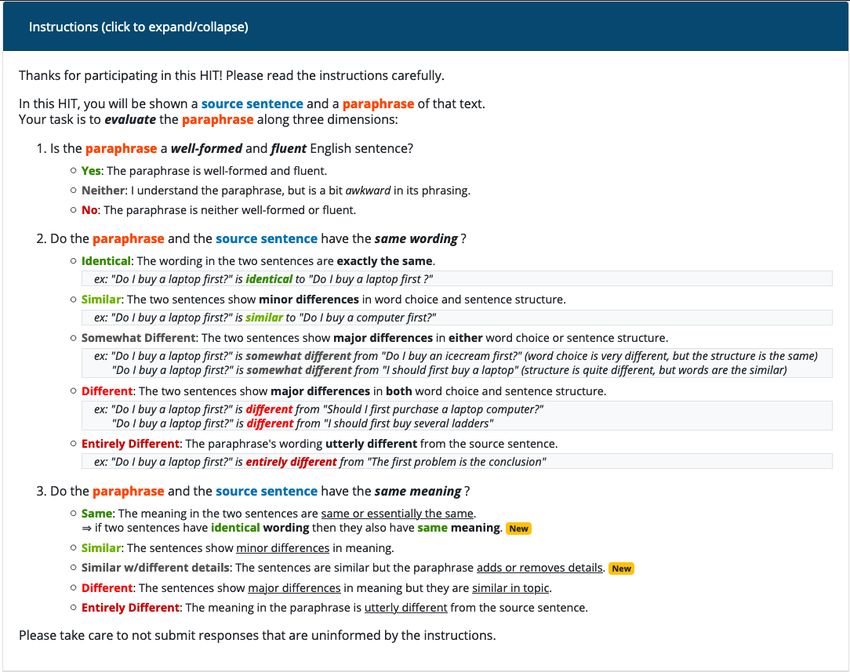
3 annotators evaluate models on 204 inputs for fluency, consistency, and novelty on Amazon Mechan-
ical Turk. The “Human” metric is the rate that examples meet the threshold for all 3: fluent enough to
understand, with at most minor differences in meaning and at least minor differences in wording. We
find rater agreement with Fleiss’ κ (Fleiss, 1971) to be 0.40 (fluency threshold), 0.54 (consistency
threshold), 0.77 (novelty threshold) and 0.48 (meets all thresholds) indicating moderate to substantial
agreement (Landis & Koch, 1977). Human evaluation is described more in §C.2.
Baselines: Parameters for R EFLECTIVE D ECODING are given in §B.4. We mainly compare against
2 unsupervised baselines: Controlled Sentence Generation by Metropolis Hastings (CGMH from
Miao et al. (2019)), and the residual VQ-VAE of Roy & Grangier (2019b) (R-VQVAE). This is a
cross-section of recent approaches (VAE, editing).
We also compare against a machine-translation approach (see Sec 5), by pivoting through German
using Transformer (Vaswani et al., 2017) models trained on WMT19 data (Barrault et al., 2019). MT
has access to bilingual data, and many past unsupervised paraphrasing works do not compare against
it. Thus, we include it in a separate section in our results, Table 1.
We include supervised baselines: the pointer generator trained by imitation learning (PG-IL) as in Du
& Ji (2019), the diversity-promoting DiPS model (Kumar et al., 2019), and a finetuned BART (Lewis
et al., 2019) model, which uses a more complex pretraining method than our LMs. Note that DiPS
generates multiple diverse paraphrases so we pick one at random.
CGMH and R EFLECTIVE D ECODING both return multiple ranked paraphrases. We can easily control
for N ovelty by taking the highest-ranked output that meets a N ovelty threshold. For each, we have
a version with no threshold (T op), and with thresholds such that average N ovelty is 30 and 45.
3.2 TASK : A BDUCTIVE NLG
Task: The Abductive natural language generation task (αNLG) presented in Bhagavatula et al.
(2020) requires generating a hypothesis that fits between observations o1 and o2 , and explains them.
We apply R EFLECTIVE D ECODING to this problem as outlined in §2.6, using available data splits.
Baselines: Parameters for R EFLECTIVE D ECODING are given in §B.4. We include baselines from
the original work: different supervised variants of GPT2 large with access to the observations, and
7Under review as a conference paper at ICLR 2021
optionally COMET (Bosselut et al., 2019) embeddings or generations. We include an unsupervised
baseline of GPT2 conditioned on o1 + o2 directly.
Metrics: For human evaluation, over 1000 examples we ask 3 raters on Amazon Mechanical Turk
about agreement between h and o1 , o2 , both, and overall quality on 4-value likert scales. We found
Fleiss’ kappa (Fleiss, 1971) of 0.31, 0.29, 0.28, and 0.30 respectively, indicating fair agreement
(Landis & Koch, 1977).
4 R ESULTS AND D ISCUSSION
Paraphrasing: On automatic metrics from past works (BLEU, METEOR, TERP ) our lowest-
N ovelty model setting (RDT op ) achieves the highest unsupervised scores, and highest overall on
BLEU. Other high scoring rows (Source, PG-IL) have similarly low-N ovelty outputs . The SARI
metric explicitly balances novelty (i.e. difference from the source) with correctness (i.e. similarity to
the reference). On SARI we see such low-N ovelty models perform worse. The best overall model
on SARI is our medium-N ovelty setting (RD30 ) which outperforms MT and supervised models.
Ultimately, human annotation is the only way to validate the results of other metrics. Our human
evaluation measures what fraction of outputs are found to be fluent, consistent, and novel. As with
SARI, both our mid and high-N ovelty models perform quite well. Our medium-N ovelty setting
RD30 achieves the highest score overall (63.1), slightly higher than RD45 (61.1) and MT (59.3).
Further, our human evaluation validates SARI as a reasonable proxy, as they share the same top-5
models.
R EFLECTIVE D ECODING is able to compete on previously used quality metrics that favor low-
N ovelty, but can easily produce more varied outputs preferred by humans. RD45 exceeds the novelty
of even the human reference, but is still among the highest ranked models by SARI and Human.
αNLG: Results on αNLG (table 2) present a strong case that R EFLECTIVE D ECODING can effec-
tively use bidirectional context. Strong hypotheses use information from both the initial observation
o1 and the future observation o2 . Humans ranked the ability of R EFLECTIVE D ECODING to cap-
ture this 0.44, about 25 points above the unsupervised baseline and only 10 points below the best
supervised method tested. We see similar results for overall evaluation.
We also include example generations in figure 2 to demonstrate the ability of R EFLECTIVE D ECODING
to combine o1 and o2 . For example, He put her on the swing, and while she was on the swing, she
fell off and was lying on the ground. incorporates information from both observations. Specifically, it
takes into account the swing that Ray is building for his daughter which is only mentioned in o1 , and
hypothesises about a potential injury due to Ray checking on his daughter in o2 .
Overall, the strong performance of R EFLECTIVE D ECODING on αNLG verifies applications beyond
paraphrasing. Indeed, all that was required to apply R EFLECTIVE D ECODING was a source text
whose content the generation should adhere to (o1 and o2 in this case), and two unidirectional LMs.
5 R ELATED W ORK
Decoding Techniques Holtzman et al. (2020) present nucleus sampling, a decoding technique to
improve generation quality. It utilized distribution truncation at the token level. When generating
a token at position i (given context x1:i−1 ), nucleus sampling operates by keeping the smallest
vocabulary Vp set that satisfies:
X
P (x|x1:i−1 ) ≥ p
x∈Vp
where p is the sampling parameter and P is the generating distribution, which is then renormalized
to the reduced vocabulary. Rather than methods like tok-k sampling which take a static number of
most-likely samples, nucleus sampling takes a static segment of the probability mass, p. Nucleus
sampling is orthogonal to R EFLECTIVE D ECODING, which instead extends LM decoding to a new set
of problems and in fact includes nucleus sampling as a subroutine. Kajiwara (2019) use a constrained
decoding scheme to improve paraphrasing, but require a supervised system.
8Under review as a conference paper at ICLR 2021
Distributional Intuitions A key aspect of R EFLECTIVE D ECODING is using a distributional
intuition to represent the meaning of a text through many contexts. Kiros et al. (2015); Miao et al.
(2019) quantify semantic and Lin & Pantel (2001) identify paraphrastic relationships under similar
intuitions. A major point of difference between past work and ours is that we generate explicit
contexts to represent meaning, allowing unsupervised generation back from representations, while
past work typically attempts to compress the full contextual distribution into a fixed-length vector.
Unsupervised Paraphrasing One ap-
proach trains neural variational auto-
o1 o2 o1 + o2 all
encoders unsupervised to represent source
sentences, then decodes from these repre- human 86.7 84.3 78.0 83.8
sentations to paraphrase (Roy & Grang-
Supervised
ier, 2019a; Bao et al., 2019). This
requires training specialized representa- COMeTEmb +GPT2 72.4 61.9 55.1 60.1
tions, whereas R EFLECTIVE D ECODING COMeTTxt +GPT2 72.1 60.3 54.6 59.4
applies general-purpose LMs. We com- O1 -O2 -Only 72.5 61.6 55.7 60.9
pare against Roy & Grangier (2019a). Unsupervised
Paraphrasing by editing the input (Miao GPT2-Fixed 24.2 21.0 18.5 19.3
et al., 2019; Liu et al., 2019) has shown Reflect Decoding 56.7 55.3 46.2 50.0
promise. Like R EFLECTIVE D ECODING,
these approaches can be applied without Table 2: Model performance on αNLG. The first 3 scores
training specialized models , but are neces- query agreement between hypothesis and given observa-
sarily limited by edit-paths and local min- tion(s), and “all” indicates overall judgement.
ima, as edits are often restricted to single-
word replacement, insertion, and deletion.
R EFLECTIVE D ECODING and MT-bases paraphrasing both pivot through an alternative textual form
to paraphrase (context and translation, resp.). But MT paraphrase systems cycle-translate through
a pivot language (Federmann et al., 2019; Wieting & Gimpel, 2018), which requires supervised
bilingual translation data, with an implicit notion of cross-lingual paraphrasing.
Novelty in Paraphrasing Mao & Lee (2019) observe that paraphrases close to the source often win
on automatic quality metrics. However, dissimilarity from the source seems to correlate with human
notions of paraphrasing (Liu et al., 2010), necessitating more nuanced metrics. Alternative metrics
that consider novelty alongside quality have previously been used (Sun & Zhou, 2012; Federmann
et al., 2019). The SARI metric (Xu et al., 2016), included here, combines these notions into a single
metric. Kumar et al. (2019) increase novelty through their diversity-promoting sampling method.
6 C ONCLUSIONS
We present R EFLECTIVE D ECODING, a novel unsupervised text generation method for tasks that do
not fit the left-to-right generation paradigm. R EFLECTIVE D ECODING uses two language models to
generate contexts that collectively represent the meaning of input text. It significantly outperforms
unsupervised baselines in quality and diversity for paraphrasing. Further, in abductive natural
language generation it outperforms the unsupervised baseline by a wide margin and closes the gap
with supervised models. R EFLECTIVE D ECODING introduces the concept of using generated contexts
to represent meaning, opening up new possibilities for unsupervised conditional text generation.
R EFERENCES
Yu Bao, Hao Zhou, Shujian Huang, Lei Li, Lili Mou, Olga Vechtomova, Xinyu Dai, and Jiajun Chen.
Generating sentences from disentangled syntactic and semantic spaces. In Proceedings of the 57th
Annual Meeting of the Association for Computational Linguistics, pp. 6008–6019, 2019.
Loı̈c Barrault, Ondřej Bojar, Marta R Costa-Jussà, Christian Federmann, Mark Fishel, Yvette
Graham, Barry Haddow, Matthias Huck, Philipp Koehn, Shervin Malmasi, et al. Findings of
the 2019 conference on machine translation (wmt19). In Proceedings of the Fourth Conference
9Under review as a conference paper at ICLR 2021
on Machine Translation (Volume 2: Shared Task Papers, Day 1), pp. 1–61, 2019. URL http:
//www.aclweb.org/anthology/W19-5301.
Chandra Bhagavatula, Ronan Le Bras, Chaitanya Malaviya, Keisuke Sakaguchi, Ari Holtzman,
Hannah Rashkin, Doug Downey, Scott Yih, and Yejin Choi. Abductive commonsense reasoning.
ICLR, 2020.
Antoine Bosselut, Hannah Rashkin, Maarten Sap, Chaitanya Malaviya, Asli Celikyilmaz, and Yejin
Choi. Comet: Commonsense transformers for automatic knowledge graph construction. In
Proceedings of the 57th Annual Meeting of the Association for Computational Linguistics, pp.
4762–4779, 2019.
Tom B Brown, Benjamin Mann, Nick Ryder, Melanie Subbiah, Jared Kaplan, Prafulla Dhariwal,
Arvind Neelakantan, Pranav Shyam, Girish Sastry, Amanda Askell, et al. Language models are
few-shot learners. arXiv preprint arXiv:2005.14165, 2020.
David Chen and William Dolan. Collecting highly parallel data for paraphrase evaluation. In
Proceedings of the 49th Annual Meeting of the Association for Computational Linguistics: Hu-
man Language Technologies, pp. 190–200, Portland, Oregon, USA, June 2011. Association for
Computational Linguistics. URL https://www.aclweb.org/anthology/P11-1020.
Michael Denkowski and Alon Lavie. Meteor universal: Language specific translation evaluation for
any target language. In Proceedings of the ninth workshop on statistical machine translation, pp.
376–380, 2014.
Wanyu Du and Yangfeng Ji. An empirical comparison on imitation learning and reinforcement
learning for paraphrase generation. In EMNLP/IJCNLP, 2019.
Christian Federmann, Oussama Elachqar, and Chris Quirk. Multilingual whispers: Generating
paraphrases with translation. In Proceedings of the 5th Workshop on Noisy User-generated Text
(W-NUT 2019), pp. 17–26, Hong Kong, China, November 2019. Association for Computational
Linguistics. doi: 10.18653/v1/D19-5503. URL https://www.aclweb.org/anthology/
D19-5503.
John R Firth. A synopsis of linguistic theory, 1930-1955. Studies in linguistic analysis, 1957.
Joseph L Fleiss. Measuring nominal scale agreement among many raters. Psychological bulletin, 76
(5):378, 1971.
Aaron Gokaslan and Vanya Cohen. Openwebtext corpus, 2019. URL http://Skylion007.
github.io/OpenWebTextCorpus.
Geoffrey E Hinton. Training products of experts by minimizing contrastive divergence. Neural
computation, 14(8):1771–1800, 2002.
Ari Holtzman, Jan Buys, Maxwell Forbes, and Yejin Choi. The curious case of neural text degenera-
tion. ICLR, 2020.
Tomoyuki Kajiwara. Negative lexically constrained decoding for paraphrase generation. In Proceed-
ings of the 57th Annual Meeting of the Association for Computational Linguistics, pp. 6047–6052,
2019.
Maurice G Kendall. A new measure of rank correlation. Biometrika, 30(1/2):81–93, 1938.
Ryan Kiros, Yukun Zhu, Russ R Salakhutdinov, Richard Zemel, Raquel Urtasun, Antonio Torralba,
and Sanja Fidler. Skip-thought vectors. In Advances in neural information processing systems, pp.
3294–3302, 2015.
Ashutosh Kumar, Satwik Bhattamishra, Manik Bhandari, and Partha Talukdar. Submodular
optimization-based diverse paraphrasing and its effectiveness in data augmentation. In NAACL-
HLT, 2019.
10Under review as a conference paper at ICLR 2021
Wuwei Lan, Siyu Qiu, Hua He, and Wei Xu. A continuously growing dataset of sentential paraphrases.
In Proceedings of The 2017 Conference on Empirical Methods on Natural Language Processing
(EMNLP), pp. 1235–1245. Association for Computational Linguistics, 2017. URL http://
aclweb.org/anthology/D17-1127.
J Richard Landis and Gary G Koch. The measurement of observer agreement for categorical data.
biometrics, pp. 159–174, 1977.
Mike Lewis, Yinhan Liu, Naman Goyal, Marjan Ghazvininejad, Abdelrahman Mohamed, Omer
Levy, Ves Stoyanov, and Luke Zettlemoyer. Bart: Denoising sequence-to-sequence pre-training for
natural language generation, translation, and comprehension. arXiv preprint arXiv:1910.13461,
2019.
Chin-Yew Lin. ROUGE: A package for automatic evaluation of summaries. In Text Summarization
Branches Out, pp. 74–81, Barcelona, Spain, July 2004. Association for Computational Linguistics.
URL https://www.aclweb.org/anthology/W04-1013.
Dekang Lin and Patrick Pantel. Dirt@ sbt@ discovery of inference rules from text. In Proceedings
of the seventh ACM SIGKDD international conference on Knowledge discovery and data mining,
pp. 323–328, 2001.
Chang Liu, Daniel Dahlmeier, and Hwee Tou Ng. Pem: A paraphrase evaluation metric exploiting
parallel texts. In Proceedings of the 2010 Conference on Empirical Methods in Natural Language
Processing, pp. 923–932, 2010.
Xianggen Liu, Lili Mou, Fandong Meng, Hao Zhou, Jie Zhou, and Sen Song. Unsupervised
paraphrasing by simulated annealing. arXiv preprint arXiv:1909.03588, 2019.
Qingsong Ma, Ondřej Bojar, and Yvette Graham. Results of the wmt18 metrics shared task: Both
characters and embeddings achieve good performance. In Proceedings of the third conference on
machine translation: shared task papers, pp. 671–688, 2018.
Hongren Mao and Hungyi Lee. Polly want a cracker: Analyzing performance of parroting on
paraphrase generation datasets. In EMNLP/IJCNLP, 2019.
Pedro Henrique Martins, Zita Marinho, and André F. T. Martins. Sparse text generation, 2020.
Ning Miao, Hao Zhou, Lili Mou, Rui Yan, and Lei Li. Cgmh: Constrained sentence generation by
metropolis-hastings sampling. In Proceedings of the AAAI Conference on Artificial Intelligence,
volume 33, pp. 6834–6842, 2019.
Tomas Mikolov, Kai Chen, Greg S. Corrado, and Jeffrey Dean. Efficient estimation of word
representations in vector space, 2013. URL http://arxiv.org/abs/1301.3781.
Kishore Papineni, Salim Roukos, Todd Ward, and Wei-Jing Zhu. Bleu: a method for automatic
evaluation of machine translation. In Proceedings of the 40th annual meeting on association for
computational linguistics, pp. 311–318. Association for Computational Linguistics, 2002.
Alec Radford, Jeffrey Wu, Rewon Child, David Luan, Dario Amodei, and Ilya
Sutskever. Language models are unsupervised multitask learners, 2019. URL
https://d4mucfpksywv.cloudfront.net/better-language-models/
language_models_are_unsupervised_multitask_learners.pdf. Unpub-
lished manuscript.
Aurko Roy and David Grangier. Unsupervised paraphrasing without translation. In ACL, 2019a.
Aurko Roy and David Grangier. Unsupervised paraphrasing without translation. In Proceedings of
the 57th Annual Meeting of the Association for Computational Linguistics, pp. 6033–6039, 2019b.
Hubert JA Schouten. Nominal scale agreement among observers. Psychometrika, 51(3):453–466,
1986.
Thibault Sellam, Dipanjan Das, and Ankur P. Parikh. Bleurt: Learning robust metrics for text
generation. In ACL, 2020.
11Under review as a conference paper at ICLR 2021
Matthew G Snover, Nitin Madnani, Bonnie Dorr, and Richard Schwartz. Ter-plus: paraphrase,
semantic, and alignment enhancements to translation edit rate. Machine Translation, 23(2-3):
117–127, 2009.
Hong Sun and Ming Zhou. Joint learning of a dual SMT system for paraphrase generation. In
Proceedings of the 50th Annual Meeting of the Association for Computational Linguistics (Volume
2: Short Papers), pp. 38–42, Jeju Island, Korea, July 2012. Association for Computational
Linguistics. URL https://www.aclweb.org/anthology/P12-2008.
Ashish Vaswani, Noam Shazeer, Niki Parmar, Jakob Uszkoreit, Llion Jones, Aidan N Gomez, Łukasz
Kaiser, and Illia Polosukhin. Attention is all you need. In Advances in neural information
processing systems, pp. 5998–6008, 2017.
Sean Welleck, Ilia Kulikov, Stephen Roller, Emily Dinan, Kyunghyun Cho, and Jason Weston. Neural
text generation with unlikelihood training. arXiv preprint arXiv:1908.04319, 2019.
John Wieting and Kevin Gimpel. Paranmt-50m: Pushing the limits of paraphrastic sentence embed-
dings with millions of machine translations. In Proceedings of the 56th Annual Meeting of the
Association for Computational Linguistics (Volume 1: Long Papers), pp. 451–462, 2018.
Wei Xu, Courtney Napoles, Ellie Pavlick, Quanze Chen, and Chris Callison-Burch. Optimiz-
ing statistical machine translation for text simplification. Transactions of the Association
for Computational Linguistics, 4:401–415, 2016. doi: 10.1162/tacl a 00107. URL https:
//www.aclweb.org/anthology/Q16-1029.
Rowan Zellers, Ari Holtzman, Hannah Rashkin, Yonatan Bisk, Ali Farhadi, Franziska Roesner, and
Yejin Choi. Defending against neural fake news. In Advances in Neural Information Processing
Systems, pp. 9051–9062, 2019.
Tianyi Zhang, V. Kishore, Felix Wu, Kilian Q. Weinberger, and Yoav Artzi. Bertscore: Evaluating
text generation with bert. ArXiv, abs/1904.09675, 2020.
A A PPENDIX
A.1 D ERIVATION OF S AMPLING F UNCTION
Here we derive the sampling function used for R EFLECTIVE D ECODING, working from a definition
of similarity based on context and deriving a function that allows generation. This section is meant to
supplement and expand upon §2.7.
To begin, for correctness we use the notation Pc|s to denote the distribution of contexts c for source
sentence s. In practice, this will be 1-sided context, for instance right-hand context crh . In this case,
−→
Pc|s would be estimated by the left-to-right language model conditioned on s: LM(c|s). A clarifying
example is included in figure 1 where contexts are sampled from this distribution.
The reverse distribution Ps|c is the opposite: going back from context towards text. With right-hand
←−
context, this is estimated by the the reverse language model LM(s|c). We will begin by using the
more general notation (Pc|s , Ps|c ) while considering theoretical quantities, then transition to using
−→ ←−
the language model distributions (LM,LM) when we are estimating these quantities in practice.
In §2.7, we consider the task of comparing a source sentence ssrc with another sentence ŝ. For
instance, we may want to know if ŝ is a paraphrase of ssrc . Following a distributional intuition
(Firth, 1957) that text with similar meaning will appear in similar contexts, we define a simple way to
compare meaning
DKL (Pc|ssrc , Pc|ŝ ) (9)
Where DKL is the Kullback–Leibler measuring the difference between the distributions Pc|ssrc and
Pc|ŝ . This is a simple way to capture a notion above: we take the amount the contexts of ssrc and ŝ
differ as a proxy for their difference in meaning and connotation.
12Under review as a conference paper at ICLR 2021
While this equation (9) plays the same role as equation 5 in §2.7, we use the LM notation in that case,
for simplicity and because we are only considering single-sided context there. Equation 9 is more
general.
In a generation setting, we are most interested in selecting for contextual closeness, and therefore
only need to rank between options. Therefore we will instead be working with the cross-entropy:
−→ −→ X −→
H(LM(c|ssrc ), LM(c|ŝ)) = −LM(c|ssrc )log(Pc|ŝ (c)) (10)
c
which is equivalent to DKL up to a constant offset, and will be easier to estimate in practice. Here,
the sum over c indicates a sum over every possible context c. In practice we will use a finite sample
estimate, but will use the theoretical formulation for now.
As stated in Sec 2.7, we are using this as a measure of contextual difference in meaning. For the
purposes of paraphrasing, we are trying to find a sentence ŝ that minimizes this, which is equivalent
to maximizing the exponent of its negation:
P
Score(ŝ) = e c −Pc|s log(Pc|ŝ (c))
Y
= Pc|ŝ (c)Pc|s (c)
c
Y Pŝ|c (ŝ)P (c) Pc|s (c)
=
c
P (ŝ) (11)
Y Pc|s (c)
Pŝ|c (ŝ)
= a0
c
P (ŝ)
a0 Y
= Pŝ|c (ŝ)Pc|s (c)
P (ŝ) c
Note, a0 is a constant factor resulting from factors of P (c). We drop this for optimization. Also, Pŝ|c
simply gives the distribution of text given context c e.g. if c is right context, this is the distribution
estimated by a R2L LM conditioned on c.
The result of derivation 11 fits the Product of Experts model of Hinton (2002). In theory, the factor of
P (ŝ)−1 will prioritize more context-specific paraphrases as a low probability sentence that’s likely
in contexts for s is more related than a sentence that’s generally likely (i.e. generic), but this has a
few issues. For one, our estimators (language models) are not well equipped to handle very unlikely
text, as they’re trained on the real distribution and so spend relatively little capacity on very unlikely
sequences. Second, while a less likely sentence can have higher similarity for the reasons stated
above, this may not be the goal of our system.
In a real setting, we are interested in related sentences that are also fluent and reasonable. For
this reason, we drop the P (ŝ)−1 term when calculating our approximate score, the equivalent of
multiplying in P (ŝ) which is simply biasing the model towards likely sequences.
This gives an augmented score:
Y
Score(ŝ) = c0 Pŝ|c (ŝ)Pc|s (c) (12)
c
Optimizing this is equivalent to taking a product of experts of the following form:
Y
Score(ŝ) = Pŝ|c (ŝ)wc|s (13)
c
There is then the question of how we should set the weights wc|s in the limited sample setting. In
the full setting, these weights are a set of probabilities Pc|ssrc (c) summing to 1 over all contexts c.
13Under review as a conference paper at ICLR 2021
This indicates the logarithm of the score corresponds to a convex combination of the logits of the
distributions Pŝ|c (ŝ). To keep in line with this notion, we will also enforce that weights constitute a
proper distribution.
In the limiting case with unlimited samples, these weights should be set to the probability of context
given s, Pc|s (c). A simple method to take this to the finite-sample case would be simply renormalizing
these probabilities given over the sampled contexts. However, it is not clear that these are the most
efficient weights for a good estimate of the scoring function. Further, while pretrained LMs are strong
estimators, exponentiating by their estimates will magnify any errors they make. Instead, we learn
these weights using a heuristic, discussed later.
As we transition to the finite-sample-setting and consider estimating this in practice, we replace
the theoretical distributions with estimates using language models. In doing so, we go from a
more general notion of context to 1-sided. Here we will consider right-context (meaning Pŝ|c is
←−
estimated by LM) but the left-context case proceeds symmetrically. Substituting in the language
model distribution:
Y ←−
Score(ŝ) = LM(ŝ|c)wc|s (14)
c
Where now the product over c indicates product over the finite sampled contexts. We will discuss
how the weights are learned, but first we convert this to a sampling function. We can now decompose
the scoring function into tokens of generation ŝ = ŝ0 ...ŝn :
Y Y ←−
Score(ŝ0:n ) = LM(ŝj |ŝj+1:n )wc|ŝ (15)
j c
This is simply restating equation 13 but factorizing LM probability by tokens.
Renormalizing and decomposing by token position, this gives a natural distribution to sample from:
Q ←−
LM(ŝj |hatsj+1:n )wc|s
Psample (ŝj |ŝj+1:n ) = P c Q ←− (16)
wc|s
t∈V c LM(t|hatsj+1:n )
Simply, we are normalizing at each point over tokens in the vocabulary V , making this a proper
token-wise distribution to sample from. Note that we are sampling right-to-left, so from index n
←−
down, to match convention. This is the sampling function referred to as RD in the body of the paper,
and state in equation 7. We use this to sample candidate generations that encourage adherence to the
semantic scoring function. Note, in practice we refer to contexts by index i (ci ) and the associated
weight as wi .
Finally, we learn the weights, following the convex combination constraint (weights are nonnegative,
summing to 1), to match one fundamental aspect of the scoring function. That is, ssrc should
receive the highest score (or similarly, should have the lowest contextual difference with itself). So
essentially, we learn weights that maximize the score/probability of ssrc , using a gradient-based
learning algorithm to achieve this. This assures that the entire algorithm can proceed using only the
two language models and input, as the signal for learning comes only from the self-generated context
and input.
B I MPLEMENTATION D ETAILS
B.1 L EFT- TO -R IGHT R EFLECTIVE D ECODING SAMPLING FUNCTION
−→
As mentioned in §2.3, a left-to-right R EFLECTIVE D ECODING sampling function RD is learned in a
←− −→ ←−
similar manner to RD, simply by switching the roles of LM and LM in algorithm 1. For completeness
we elaborate on this here.
First, the roles of the language models are flipped in the sampling function:
14Under review as a conference paper at ICLR 2021
Algorithm 2: Learn R EFLECTIVE D ECODING sampling function (left-to-right)
−→
Input: Left to right language model LM
←−
Right to left language model LM
Source text: ssrc
←−
1: Sample contexts, c1 ...cnc ∼ LM(c|ssrc )
P
2: Initialize parameters w = w1 ...wnc s.t. wi = 1, wi ≥ 0
−→ Q −→
3: RD(s) ∝ i LM(s|ci )wi normalized by token (equation 17)
−→
4: learn w = arg
P maxw RD(ssrc )
under wi = 1, wi ≥ 0
−→
Output: RD
Q −→ wi
−→ i LM(s|ci )
RD (s) = Q|s| P Q −→ (17)
wi
j=0 t∈V i LM(t|s0:j−1 + ci )
←−
where contexts ci are now generated by the backwards language model LM (i.e. left-contexts). We
−→
then present algorithm 2, which defines how to learn RD.
B.2 P OST- PROCESSING G ENERATIONS
Without learning stop-tokens, R EFLECTIVE D ECODING samples fixed number (lenŝ ) of tokens.
Candidates are extracted from raw generations using a combination of sentence tokenization to trim
extra text to the sentence boundaries.
B.3 E NTROPY C ALIBRATION
Entropy calibration is used when sampling candidate generations (§2.4). We expand on the earlier
definition here.
When sampling output generations, generation parameters (nucleus sampling pŝ in paraphrasing)
control how “greedy” or stochastic the sampling process is. However, the exact effect of a specific
value of pŝ depends on target length, number of generated contexts, complexity of meaning, desired
level of agreement with source etc. Setting pŝ too low may sample only the most likely option, but too
high can result in off-topic candidates. Simply, the “correct” value of pŝ is highly sample-dependent.
Instead, we define a technique, entropy calibration, designed to control how much “randomness” is
used in sampling in a more robust way. Rather than directly setting a pŝ for all examples, entropy
calibration allows the user to specify the amount of randomness or approximate entropy ĥ they would
like to sample with over each example. In the greedy case for instance, the desired entropy ĥ is set to
0, or equivalently we are picking from a set of 1 possible option. Likewise, the user might set ĥ to 4,
which would result in a higher pŝ (how much higher will be example-dependant).
In practical terms, we search for pŝ in each case that is expected to give the correct level of “random-
ness” over the entire generation, although pŝ is a token-level parameter. To estimate how random
a given value of pŝ will make a generated sentence, we take the sampling entropy over the source
string s0 ...sn under the nucleus-sampling truncated distribution Pp :
X X
ĥ = −Pp (w|s0 ...si−1 )logPp (w|s0 ...si−1 )
i w∈Vp
Where Vp is the truncated vocabulary with parameter p. Roughly, this captures a branching-factor
over the sequence. We select pŝ that gives a desired entropy. We set this to values of 4 or 6 which we
found effective. Parameters are available in App. B.4.
15Under review as a conference paper at ICLR 2021
Param Paraphrasing αNLG
model size Mega Mega
lenŝ or lenh len(s) + 5 20
lenc 50 50
nŝ 30 20
nc 80 50
hsample 4. 6.
pc 0.7 0.9
kc 6 6
Table 3: Most parameters are explained in §2.4. hsample is entropy for sampling calibration in §B.3
B.4 PARAMETERS
In this section, we outline model settings for our 2 experimental settings, paraphrasing and αNLG.
See Table 3.
Broadly, αNLG achieves higher variety in output with a higher sampling entropy (hsample ), more
diverse generated contexts (higher pc ), and fewer generated contexts (nc ).
To find these parameters, we experimented with different reasonable values on the dev set of each
model, and evaluated manually whether generated text appeared reasonable, specifically reading
examples and picking model settings that produced good paraphrases as judged by the authors. For
lenŝ and lenh we simply set this high enough to ensure desirable outputs would be a subsequence.
We trained our transformer language models on TPU pods (using code in TensorFlow) of size 512
until convergence. During our generation experiments, we transferred the model to Pytorch, and ran
locally on a machine with 2 NVIDIA Titan Xp GPUs.
C E VALUATION
C.1 AUTOMATIC M ETRICS
Links to the code we used for automatic evaluation is given here:
• ROUGE
• BLEU
• METEOR
• TERP
• SARI
• BERTScore
• BLEURT
We include a limited number of metrics in the main paper for space and clarity, but include fur-
ther metrics tested in table 4: ROUGE-1, ROUGE-2 (Lin, 2004), BLEURT Sellam et al. (2020),
BERTScore (Zhang et al., 2020). For BLEURT, we used the ”BASE” pretrained model suggested by
the authors. For BERTScore, we use the default settings of the official codebase.
C.2 H UMAN E VALUATION
For human evaluation in paraphrasing, we evaluate on 204 input sentences, having 3 raters evaluate
each model’s output. We ask about fluency, consistency with the source, and difference in wording
from the source (template in figure 4). In each case, we use a multi-point likert scale, but are mainly
interested in whether generations meet a threshold for each criterion: fluent enough to understand,
with at most minor differences in meaning and at least minor differences in wording. In table 5 we
give the rate for each model that humans found the generation meets these thresholds. The “Overall”
column is the rate that humans find generations meet all 3 measured criteria. We take Fleiss’ κ on
16You can also read