Dynamic in Species Estimates of Carnivores (Leopard Cat, Red Fox, and North Chinese Leopard): A Multi-Year Assessment of Occupancy and Coexistence ...

Page created by Janet Mcguire
 
CONTINUE READING
Dynamic in Species Estimates of Carnivores (Leopard Cat, Red Fox, and North Chinese Leopard): A Multi-Year Assessment of Occupancy and Coexistence ...
animals
Article
Dynamic in Species Estimates of Carnivores (Leopard
Cat, Red Fox, and North Chinese Leopard):
A Multi-Year Assessment of Occupancy and
Coexistence in the Tieqiaoshan Nature Reserve,
Shanxi Province, China
Kasereka Vitekere 1,2 , Jiao Wang 1 , Henry Karanja 1,3 , Kahindo Tulizo Consolée 1 ,
Guangshun Jiang 1, * and Yan Hua 4, *
 1   Feline Research Center of National Forestry and Grassland Administration, College of Wildlife and Natural
     Protected Area, Northeast Forestry University, Harbin 150040, China; vitekere@nefu.edu.cn (K.V.);
     wj15765526221@163.com (J.W.); hkaranja@egerton.ac.ke (H.K.); tulizok@yahoo.com (K.T.C.)
 2   Department of Natural Resources, Egerton University, P.O. Box 536-20115 Egerton, Kenya
 3   Tayna Center for Conservation Biology, University of Nature Conservation and Development at Kasugho,
     Goma 167, North-Kivu, Democratic Republic of Congo
 4   Guangdong Provincial Key Laboratory of Silviculture, Protection and Utilization, Guangdong Academy of
     Forestry, Guangzhou 510520, China
 *   Correspondence: jgshun@126.com (G.J.); wildlife530@hotmail.com (Y.H.)
                                                                                                      
 Received: 7 July 2020; Accepted: 28 July 2020; Published: 1 August 2020                              

 Simple Summary: Carnivores are among the threatened mammal species due to interactions with
 humans and environmental effects. We collected data using camera traps across three sampling
 periods over three years, aiming to study the coexistence mechanisms of three carnivores: the North
 Chinese leopard, the leopard cat, and the red fox to depict effects from an environmental factor and
 anthropogenic disturbances on these carnivores within a landscape. The occupancy modeling showed
 that all species’ occupancy did not greatly change across years and they rather depicted occupancy
 stability. The elevation impacted more on species’ occupancy estimates than distances to villages and
 roads. We performed a multi-year assessment of species’ estimates and the results of this study reveal
 the impact of habitat features and anthropogenic disturbances on the occupancy dynamics of the
 North Chinese leopard, the red fox and the leopard cat in the Tieqiaoshan nature reserve landscape.

 Abstract: Wildlife populations are spatially controlled and undergo frequent fluctuations in abundance
 and site occupation. A comprehensive understanding of dynamic species processes is essential for
 making appropriate wildlife management plans. Here, we used a multi-season model to describe the
 dynamics of occupancy estimates of the carnivores: North Chinese leopard (Panthera pardus japonensis,
 Gray, 1862), leopard cat (Prionailurus bengalensis, Kerr, 1792), and red fox (Vulpes vulpes, Linnaeus,
 1758) in the Tieqiaoshan Nature Reserve, Shanxi Province, China, over a three-year study period
 using camera traps data. The occupancy probability of the North Chinese leopard did not markedly
 change with time as the occupancy equilibrium was constant or slightly enhanced. The occupancy of
 the leopard cat decreased with time. The occupancy equilibrium of the red fox alternately increased
 and decreased. However, all species presented a slight level of occupancy stability due to their small
 values of the rate of change in occupancy. Environmental factor and anthropogenic disturbances
 slightly influenced the occupancy of all species and the colonization and extirpation probability of
 the red fox. The colonization and extirpation for all species were relatively more strongly affected by
 the distances to villages and roads. Moreover, elevation increased the colonization and decreased
 the extirpation for the leopard cat. Species interaction factors increased with time for all species.
 The North Chinese leopard and the leopard cat avoided each other. The leopard cat and the red fox

Animals 2020, 10, 1333; doi:10.3390/ani10081333                                  www.mdpi.com/journal/animals
Dynamic in Species Estimates of Carnivores (Leopard Cat, Red Fox, and North Chinese Leopard): A Multi-Year Assessment of Occupancy and Coexistence ...
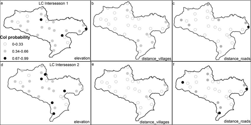
Animals 2020, 10, 1333                                                                              2 of 20

 independently co-occurred. There was true coexistence between the North Chinese leopard and the
 red fox. This research confirmed that environmental factors and human perturbations are vital factors
 to consider in wild carnivores’ conservation and management.

 Keywords: anthropogenic disturbances; colonization; environmental factor; extirpation; occupancy;
 species dynamics

1. Introduction
      In natural habitats, the abundance of a population within a habitat may fluctuate [1].
Spatiotemporal patterns are characteristic of species dynamics. Demographic parameters such
as birth and death rates and migrations modulate population distributions by alternately increasing
and decreasing the number of individuals [2,3]. Therefore, the use of the site by the population varies
with time. Indeed, spatial patterns are also crucial as habitat loss by modification and fragmentation
disrupts local cohesion and alters individual occupancy [4,5].
      Within landscapes, species may be relatively numerous at some sites and in certain habitats (forest
groves or close to the salt marshes). At other locations, however, they may be scarce (disturbed habitats
in vicinity with human activities) compared to their core distribution [1]. Wildlife managers must
prioritize habitat integrity in order to maintain the species in protected areas [6–8] and ensure longtime
wildlife presence in protected areas [9]. Effective wildlife conservation requires understanding the
mechanisms that cause population fluctuations. Site occupation is measured to determine how species
react to habitat changes caused by environmental or anthropogenic perturbations [10]. Therefore,
in wildlife management, it is essential to assess the impacts of environmental factors and anthropogenic
disturbance variations in a landscape on the viability of species.
      Most large mammals are particularly vulnerable to habitat change as they have naturally low
birth rate, are more hunted than other species, and perform large-range movements for resources [11].
Landscape changes threaten mammal occupancy and big predators such as Pathera spp. require wide
living spaces for their daily activity. In the attempt to meet their resource requirements, carnivores may
extend their activity beyond protected areas [3,12] where they might encounter human land use [13].
In China, anthropogenic threats have degraded 63–75% of leopard (Panthera pardus) habitat [14,15].
      The ecology of carnivore species has been extensively researched. These studies showed that
carnivores have a substantial impact on animal population structure in a habitat [3,16], trophic level
function [17], ecosystem resilience [18], and prey population stability [19]. Thus, ecologic studies of
carnivores are vital within an ecosystem, and carnivores site occupation is an important factor in these
studies, particularly for species distribution. The correlation between changes in local population and
the species distribution narrows the description of spatiotemporal population dynamics. Nevertheless,
elucidation of these processes is important for effective species management [20,21]. Changes in habitat
occupancy over time reliably indicate extirpation or colonization. These changes can be evaluated by
statistical models [22].
      In most habitats, sites where natural vegetation predominates are the most preferred by carnivore
populations [3]. At such locations, most native species still occur and ecological processes (predation,
niche partitioning, etc.) operate essentially unchanged [3]. Our study area, the Tieqiaoshan Natural
Reserve (TNR), is a habitat for sympatric carnivores such as the endangered North Chinese leopard
(NCL), which is endemic to China [5,23,24], a large carnivore with approximatively 32–80 kg. The NCL
should occupy specific ranges with high vegetation cover rate [25]. The areas surrounding the TNR are
adversely affected by human disturbances (land transformation, fragmentation of natural ecosystems,
implanting built up areas, infrastructure, husbandry, etc.). Consequently, carnivore population sources
in the reserve’s favorable habitat may be transformed into population sinks and destabilize carnivore
distributions within the reserve. The NCL regularly interacts with the red fox (RF) (Vulpes vulpes,
Dynamic in Species Estimates of Carnivores (Leopard Cat, Red Fox, and North Chinese Leopard): A Multi-Year Assessment of Occupancy and Coexistence ...
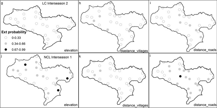
Animals 2020, 10, 1333                                                                               3 of 20

Linnaeus, 1758) and the leopard cat (LC) (Prionailurus bengalensis, Kerr, 1792), but their ecological
coexistence in this landscape remains unknown. The RF is the largest of the true foxes (2.2–14 kg),
a Least Concern species, and one of the most broadly distributed carnivorous species. RF is distributed
over the entire northern hemisphere [26], occupies various habitats, and is well adapted to human
environments. The LC is a small wild cat (2–4 kg) native to East and Southeast Asia [27]. It is also a Least
Concern species [28]. LC dwells in a wide range of natural habitats and modified areas [29]. There is a
lack of information about population numbers of all three species in this area. We assumed that as
NCL is a large carnivore, it should dominate smaller carnivores such as LC and RF. The information
derived therefrom could help develop conservation measures for these three species in the study area.
These three species were chosen in the TNR because they are the biggest carnivore species caught
in our cameras within the TNR landscape, thus they would have an essential role in the ecological
processes in the landscape, and have always been encountered in vicinity of human settlements and
roads, according to our observations. We assumed that RF would dominate the LC. Environmental
(elevation, habitat type, etc.) [12] and anthropogenic (human settlements and roads) [30,31] factors
influence the spatiotemporal dynamics of a species. Dynamic estimates for these carnivores would
be strongly correlated to environmental factors and anthropogenic disturbances. The influence of
the co-occurrence of NCL, RF, and LC may be apparent in the estimates for all three species over
time. Overlapping activity may enable a subordinate species to decrease the fitness of a dominant
species [32,33] and increase the extirpation probability [34,35].
     Several earlier multi-year assessments of species dynamics have focused mainly on occupancy,
detection, colonization, and extirpation [16,36,37]. However, they did not attempt to clarify the
mechanisms driving the rate of changes in site occupation of a species [2,38]. Some studies have used
camera trap data to estimate species dynamics by occupancy over time [39]. Here, we tested the a
priori hypothesis that both variable categories affect species estimates at different intensities over
time. To this end, we applied multi-season occupancy models with covariates to disclose how an
anthropogenic or environmental factor influences NCL, RF, and LC in their habitats.
     We examined whether the recent conservation approaches applied to protect the TNR effectively
mitigated changes in NCL, RF, and LC occupancy by reducing pressures across three years.
We hypothesized that the rate of change in occupancy fluctuate and occupancy equilibrium will
not be established for all three species. We also predicted that NCL, RF, and LC would be more
profoundly influenced by anthropogenic disturbances than environmental factor during the same
data collection period. Finally, we hypothesized that NCL, RF, and LC truly co-occurred and
spatially overlapped.

2. Materials and Methods

2.1. Study Area
     The present study was conducted at the Tieqiaoshan Nature Reserve (TNR), Shanxi Province, China
(Figure 1). The TNR is a federally protected area created in 2002 by the federal people’s administration,
allowing local population settlement in the TNR with strict measures of wildlife protection. The TNR
has more than 40 villages, with nearly 30,022 inhabitants; the density is 85 inhabitants/km2 . The total
area is 353.52 km2 ; the elevation is mainly in the range of 1300–1700 m.a.s.l., with the highest point of
1827 m.a.s.l. The area hosts a high wildlife diversity including 24 species of mammals, 6 species of
reptiles, 3 species of amphibians, and 116 species of birds. Sixteen wild animal species are protected
there [23]. The region has a typical temperate continental monsoon climate with long winters and hot
summers. The annual average temperature is almost 6 ◦ C and the daily average is 10 ◦ C [40]. The mean
annual precipitation is 560 mm. Rainfall is intense from July to September. The soil is constituted by a
mixture of sandy and stony parts. The vegetation is dominated by deciduous broadleaf, coniferous,
and mixed deciduous forests. The dominant tree species are Chinese red pine (Pinus tabuliformis),
Liaotung oak (Quercus liaotungensis), white birch (Betula platyphylla), and sparse North China larch
Dynamic in Species Estimates of Carnivores (Leopard Cat, Red Fox, and North Chinese Leopard): A Multi-Year Assessment of Occupancy and Coexistence ...
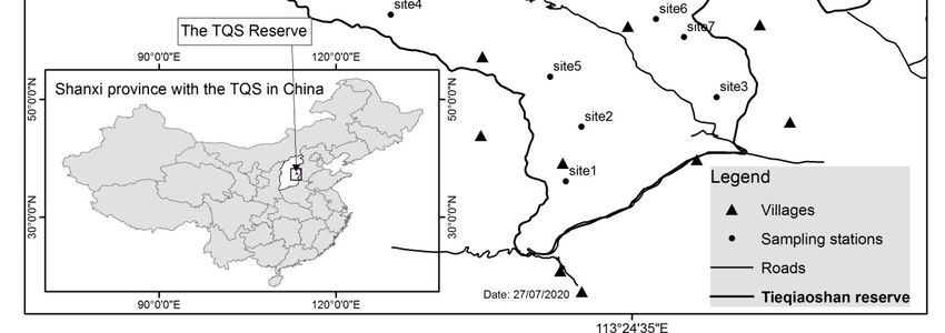
Animals 2020, 10, 1333                                                                                     4 of 20

Animals 2020, 10, x FOR PEER REVIEW                                                                        4 of 20
(Larix principis). The TNR landscape has 78 genera of wild seed plants [40] and some grassland [25].
and  some
Within  the grassland  [25]. Within
            TNR landscape,    the wildthe   TNR
                                         boar     landscape,
                                               (Sus            the wild
                                                    scrofa), Eastern      boar (Capreolus
                                                                      roe deer  (Sus scrofa), Easternand
                                                                                           pygargus), roe Cape
                                                                                                          deer
(Capreolus
hare (Lepuspygargus),  and Cape
              sp) are potential    hareof
                                 preys   (Lepus  sp) are potential
                                            the studied   carnivores,preys  of the
                                                                        mostly   thestudied carnivores,
                                                                                      NCL [23],         mostly
                                                                                                as the RF  and
the NCL [23],
LC always       as on
             prey  thesmall
                       RF and   LC always
                             mammals          prey on
                                          (Reserve     small mammals
                                                    Manager,    Unpubl. (Reserve
                                                                           data). OnlyManager,  Unpubl.
                                                                                         an overall      data).
                                                                                                    number   of
Only  an overall
mammals    is citednumber   of mammals
                    but specific             is NCL’s
                                 statistics on  cited but
                                                       main specific statistics
                                                              prey remain       on NCL’s main prey remain
                                                                             unknown.
unknown.

                  Overview of
        Figure 1. Overview of the
                              the study
                                  study area.
                                        area. Black
                                              Black dots
                                                    dots represent
                                                         represent sites
                                                                   sites where
                                                                         where camera
                                                                               camera traps were placed.

2.2. Study Design
2.2. Study Design
2.2.1. Presence/Absence Data
      This investigation was a trap-based camera study. Presence and absence data were collected along
     This investigation was a trap-based camera study. Presence and absence data were collected
with a variety of ancillary information (e.g., behavior, age, and physical characteristics). Cameras were
along with a variety of ancillary information (e.g., behavior, age, and physical characteristics).
deployed to take species’ photographs in a manner that is consistent with the sampling framework
Cameras were deployed to take species’ photographs in a manner that is consistent with the sampling
to yield data that are well suited for occupancy models [39]. Two brands of cameras were used,
framework to yield data that are well suited for occupancy models [39]. Two brands of cameras were
namely Eastern Red Hawk E1B 6210M and LTL6210MM, with only the first brand in the first
used, namely Eastern Red Hawk E1B 6210M and LTL6210MM, with only the first brand in the first
sampling period and both brands in two other sampling periods. Data were gathered for three years
(2017–2019) and corresponded to three sampling periods (seasons) with 130 (March–July 2017), 119
(September–December 2018), and 134 (March–June 2019) consecutive days, respectively. Recall that
in the occupancy model the word “season” does not necessarily mean geographic season (winter,
summer, autumn, or spring). It just means the period in which data were collected [34]. Eighty-one
cameras were used in the first sampling period and 62 were used in the second and third sampling
periods. Cameras were installed in an approximately 4 km × 4 km grid and attached to trees with
average height = 0.50 m. Two or three cameras were deployed at each sampling site and faced each
other on the animal trails [41]. The analyses were at the scale of camera trap stations rather than
other on the animal trails [41]. The analyses were at the scale of camera trap stations rather than home
home ranges, as carnivore species were likely to range between different stations during the survey
ranges, as carnivore species were likely to range between different stations during the survey period.
period. Cameras were set to capture date and time automatically; they were operated 24 h/day and the
Cameras were set to capture date and time automatically; they were operated 24 h/day and the
batteries were checked monthly. To ensure balanced sample representation at every site, each camera
operated for ≥100 consecutive days per sampling period. A species was considered to be present on a
operated for ≥100 consecutive days per sampling period. A species was considered to be present on
a sampling day if it appeared at least once in a single camera at a sampling site. To maintain temporal
independence of the captured pictures, a threshold of 30 min was used as the interval to separate two
Dynamic in Species Estimates of Carnivores (Leopard Cat, Red Fox, and North Chinese Leopard): A Multi-Year Assessment of Occupancy and Coexistence ...
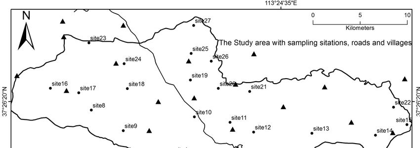
Animals 2020, 10, 1333                                                                               5 of 20

sampling day if it appeared at least once in a single camera at a sampling site. To maintain temporal
independence of the captured pictures, a threshold of 30 min was used as the interval to separate
two different observations [42]. The data processing was done within the Feline Research Center of
National Forestry and Grassland Administration of the Northeast Forestry University by experts in
Chinese carnivores who made visualization to identify species. All animal presence was recorded,
and we only used specific photographs (for three carnivore species) in this study.

2.2.2. Predictor Variables
     To formulate a fit candidate model set, predictor variables were selected according to the
observed landscape features. Three variables in two categories were collected. Elevation (el) was an
environmental variable. Distance from villages (dv) and distance from roads (dr) were spatial measures
of anthropogenic disturbances. The distance measurements were made by the proximity-near tool from
the geoprocessing analysis menu in ArcMap (ArcGIS version. 10.2.0.3348, copyright© 1999–2013 Esri
Inc. Redlands, USA, all rights reserved) after the projection of all villages and digitized roads inside
and outside the research area. Software performance was improved by standardizing the continuous
values of the variables with a z-transformation [38] as follows:
                                                      x1 − a
                                               xi =                                                     (1)
                                                        b
where xi is the new covariate value, x1 is the original observed covariate value, a is the average of all
the covariate values, and b is the standard deviation.
      To test for multicollinearity among predictor variables, Pearson’s correlation coefficient (r) was
calculated in R v. 3.5.0 [43,44]. Covariates were strongly linked when r > 0.6. The total numbers of
survey days were not equal for all seasons. Hence, data for three seasons were aggregated in the
same length periods in order to standardize the number of surveys and improve software model
computation performance [16,45]. For Seasons 1 and 3, two weeks were considered as one survey,
and for Season 2, ten days were aggregated. A species was considered to be detected if it was present
at a site in an interval of aggregated days. Otherwise, it was not detected [16,45].

2.3. Data Analysis

2.3.1. Occupancy Models
     Occupancy models were run in PRESENCE v. 5.8 (; James E. Hines, Dunedin,
New Zealand), to investigate multi-year species dynamics. Occupancy model construction varies
with the type of research hypothesis [10]. However, all models use presence/absence data as the input
and obtain specified estimates as the output. Occurrence data for targeted species were collected at
different sites within an area. As species detection was imperfect, data were collected within N sites for
T sampling occasion and species presence/absence data were recorded while checking cameras [22,38].
Occupancy models can make strong inferences about the effects of landscape fluctuations on species
site occupation [10]. These models are likelihood-based, and their estimates may be modeled as
covariate functions [46]. Thus, each sampling site was associated with the averages of various predictor
variables and their influences were modeled on the estimated species parameters.

2.3.2. Dynamic Multi-Season, Single-Species Model
     In the present study, season refers to the year wherein consecutive surveys were conducted.
A logistic model was computed according to the method of MacKenzie et al. [22]. Four parameters
that may change between years were used: (1) occupancy (psi) (probability of a site being occupied
by a species); (2) detection (p) (probability of a species being detected at a site; (3) colonization (gam)
(probability of a site being unoccupied during time t and becoming occupied at time t+1 ); and (4)
extirpation (eps) (probability of a site previously occupied during time t becoming unoccupied at time
Dynamic in Species Estimates of Carnivores (Leopard Cat, Red Fox, and North Chinese Leopard): A Multi-Year Assessment of Occupancy and Coexistence ...
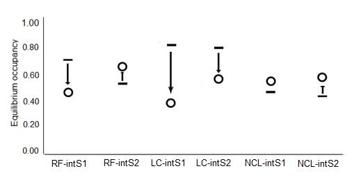
Animals 2020, 10, 1333                                                                                                   6 of 20

t+1 ) [22,46]. These parameters encompass all dynamic patterns within a habitat over the predetermined
time t+n (Figure 2), where n = different seasons.
Animals 2020, 10, x FOR PEER REVIEW                                                                                      6 of 20

      Figure
      Figure 2.
              2. Scheme
                  Schemeofofmulti-season
                              multi-seasonprocess
                                            processmodels,
                                                    models,Col, colonization;
                                                             Col,             Ext,Ext,
                                                                   colonization;   extirpation;  No No
                                                                                       extirpation; col, col,
                                                                                                          no
      colonization; No ext, no extirpation.
      no colonization; No ext, no extirpation.

    A derived parameter, the rate of change in occupancy, was performed to interpret the species
dynamics. This
          This estimate
               estimate was
                        was computed
                            computed according to MacKenzie et al. [34]:
                                                               /
                                                   ′ = ψt+1 /(1 − ψt+1 )                                                    (2)
                                                λ0t =          /                                                              (2)
                                                            ψt /(1 − ψt )
     These dynamic multi-seasons, single-species models use a strong design. Estimates (psi, p, gam,
     Theseare
and eps)     dynamic
                assumed multi-seasons,    single-species
                             to be “closed”       to changes   models     use a strong
                                                                   or movement            design.
                                                                                      during    theEstimates
                                                                                                       surveys. (psi,   p, gam,
                                                                                                                  In practice,
and eps) are
however,      assumed
            they  may be to be  “closed”
                             “open”        to changes
                                       between             or movement
                                                     seasons     [34]. Thisduring      the surveys.
                                                                               assumption               In practice,
                                                                                               introduces             however,
                                                                                                               heterogeneity,
they  may  be  “open”   between     seasons    [34].  This   assumption      introduces    heterogeneity,
which, in turn, causes estimate bias. Nevertheless, predictor variables can overcome this bias                 which,   in turn,
                                                                                                                           [22].
causes  estimate  bias.  Nevertheless,    predictor      variables    can  overcome     this
Therefore, models were constructed using different predictor variables to determine whether  bias   [22]. Therefore,    models
were constructed
estimates          using different
           across seasons             predictor variables
                              were influenced                   to determine
                                                    by year, elevation,          whether
                                                                              distance      estimates
                                                                                         from   villages,across seasons from
                                                                                                            or distance    were
influenced   by year, elevation,   distance   from    villages,   or distance   from   roads.  An
roads. An information-theoretical approach was developed to model estimates over three years. The   information-theoretical
approach
set        was developed
    of potential  models was  to model
                                 reduced estimates     over three
                                            with Akaike’s             years. TheCriterion
                                                                 Information        set of potential    models
                                                                                              (AIC) [47].        was reduced
                                                                                                             Parameters     that
withdescribed
best  Akaike’s Information       Criterion
                 the detectability    of each (AIC)    [47].per
                                                 species      Parameters
                                                                  year were that     best described
                                                                                selected.  The parametersthe detectability
                                                                                                                “specific site of
each  species  per year  were   selected.   The    parameters      “specific   site effects” and
effects” and “seasonal effects” were represented in the models by “sse” and “se”, respectively; they“seasonal   effects”   were
represented
were   used toinperform
                 the models     by “sse” and
                           detectability.   Thus,  “se”,   respectively;
                                                      predictor     variablesthey   were
                                                                                 were      used
                                                                                        used   to to  performpsi,
                                                                                                   compute       detectability.
                                                                                                                    gam, and
Thus,  predictor  variables    were  used  to   compute      psi,  gam,   and  eps,  and  the
eps, and the considered estimates were from model averages made from all the models computed.  considered     estimates    were
from  model   averages    made    from  all  the  models     computed.       This   multi-stage
This multi-stage procedure was realistic because the primary objective was not to estimate         procedure     was   realistic
because the primary
detectability.  However, objective   was was
                              detection   not to     estimate detectability.
                                                  important                         However,of
                                                                  for the determination          detection
                                                                                                     occupancywas estimation
                                                                                                                   important
for the determination     of  occupancy    estimation       values    [10,48].  Models    with  ∆AIC
values [10,48]. Models with ∆AIC ≤ 6.0 were suitable for the prediction of relevant estimate inferences. ≤  6.0 were   suitable
for the
The  2.0prediction   of relevant
         threshold was              estimate
                           too stringent        inferences.
                                            [49],   and a 6.0The cutoff2.0was
                                                                           threshold    was too
                                                                                considered     aptstringent    [49],inand
                                                                                                     [50]. Trends          a 6.0
                                                                                                                        species
cutoff was considered
occupancy     progression aptwere
                               [50]. predicted
                                      Trends in species
                                                     accordingoccupancy      progression
                                                                    to various      seasonal were    predicted
                                                                                                values.    The according
                                                                                                                 “occupancy    to
various  seasonal  values.    The  “occupancy      equilibrium”       trend  for  each
equilibrium” trend for each species was calculated following MacKenzie et al. [34]:     species  was    calculated   following
MacKenzie et al. [34]:
                                                                         γ
                                                 ψequilibrium ==                                                            (3)
                                                                                                                              (3)
                                                                     (γ + ε)
    To illustrate the influences of predictor variables on vital species estimates such as colonization
and extirpation, maps of the strong variable effects
                                              effects were
                                                      were plotted
                                                           plotted in
                                                                    in ArcGIS
                                                                       ArcGIS v.
                                                                              v. 10.2.
                                                                                 10.2.

2.3.3. Dynamic Multi-Season Co-Occurrence Model
     The co-occurrence of three carnivores was investigated over three years and multi-season, two-
species occupancy models were run. NCL was designated Species A (dominant) and LC and RF were
designated Species B (subordinate). For the second combination, RF was Species A and LC was
Species B. We computed seven co-occurrence estimates (Table 1). The φ output illustrated species
interactions within a habitat: φ < 1 indicated species avoidance, φ > 1 indicated species overlap, and
φ = 1 indicated independent species co-occurrence. The occupancy probability and vital probabilities
Animals 2020, 10, 1333                                                                                                    7 of 20

2.3.3. Dynamic Multi-Season Co-Occurrence Model
     The co-occurrence of three carnivores was investigated over three years and multi-season,
two-species occupancy models were run. NCL was designated Species A (dominant) and LC and
RF were designated Species B (subordinate). For the second combination, RF was Species A and
LC was Species B. We computed seven co-occurrence estimates (Table 1). The ϕ output illustrated
species interactions within a habitat: ϕ < 1 indicated species avoidance, ϕ > 1 indicated species
overlap, and ϕ = 1 indicated independent species co-occurrence. The occupancy probability and vital
probabilities (colonization and extirpation) in the co-occurrence model across years were selected [31,41].
Values were estimated to determine how the three aforementioned species shared this habitat. We made
a co-occurrence model with species two-by-two instead of three species together because there are still
issues to perform a multi-season–multispecies model (MacKenzie, pers. comm.)

      Table 1. Parameters interpreted from dynamic multi-season models illustrating dynamic and
      co-occurrence estimates for RF, LC, and NCL in the TNR.

         Parameters                                                    Definitions
           psiBA            The probability that Species B initially occupies the area, given that Species A is also present
           psiBa            The probability that Species B initially occupies the area, given that Species A is not present
                              The probability that Species A colonizes the area in the interseason t-(t+1 ) given that
           gamAB
                                                         Species B is present in season t
                              The probability that Species A colonizes the area in the interseason t-(t+1 ) given that
           gamAb
                                                       Species B is not present in season t
                            The probability that the area goes extinct by Species A in the interseason t-(t+1 ) given that
           epsAB
                                                          Species B is present in season t
                            The probability that the area goes extinct by Species A in the interseason t-(t+1 ) given that
           epsAb
                                                        Species B is not present in season t
           ϕ (phi)                                        Species Interactions Factor (SIF)

3. Results

3.1. Naïve Occupancy, Trap Success, and Seasonal Capture
     Surveys in the TNR generated 589, 496, and 472 independent photographs for targeted species
in Seasons 1–3, respectively. There were 10,530, 7378, and 8308 night-traps for the three respective
sampling periods. Species photographs were apportioned according to the number of cameras and
the duration of data collection per season (Table 2). However, Sampling Period 1 used more cameras
than those for Sampling Periods 2 and 3 but there were fewer photographs of LC than in the last two
sampling periods.

      Table 2. Independently captured photographs of RF, LC, and NCL in the TNR during three sampling
      seasons, including sampling period (SP); number of cameras used (nCAM); total independent
      photographs captured (TIP); number of independent photographs (nIP); survey duration representing
      total number of camera traps on field (SD); global trap success (GTS), for three species = total
      number of photographs/total number of night traps, and the total number of night traps = number of
      cameras × days of data collection; specific trap success (STS); and naïve occupancy (NO) performed by
      number of sites in which species occurred/total number of sites wherein the survey was conducted.
      Values in bold font are highest in category.

                                                                Fox                  Leopard Cat              Leopard
    SP      nCAM TIP          SD (days)    GTS (%)
                                                        nIP    STS       NO     nIP     STS     NO      nIP     STS      NO
   One       81       589        130         5.60       410     3.90     0.74   108     1.02    0.77     71     0.67     0.44
   Two       62       496        119         6.72       308     4.17     0.60   135     1.82    0.55     53     0.71     0.37
   Three     62       472        134         5.68       259     3.11     0.66   148     1.78    0.70     65     0.78     0.40
Animals 2020, 10, 1333                                                                                  8 of 20

3.2. Multi-Year Estimates and Variable Effects
      We fitted eight models for RF and nine models each for LC and NCL. All models strongly
upheld our inferences. Specific site effects and seasonal effects explained variations in detection
probability because models with p(sse) [38] and p(se) in detection computation had lower ∆AIC
than those with both variables. All models had ∆AIC that were inferior to the cutoff we selected
(Table 3). For RF, the model with the lowest ∆AIC was psi(.)gam(year),eps(year),p(sse). For LC, it was
psi(.),gam(.),eps(year+dr),p(se). For NCL, it was psi(year+dr),gam(year+dr),p(se).

      Table 3. Top-ranking candidate models for multi-season occupancy analysis for RF, LC, and NCL
      including AIC values (AICs), delta AIC (∆AIC), AIC weight (W), model likelihood (ML), number of
      parameters (K), and −2LogLike (−2L).

                     Models                     AICs     ∆AIC    W         ML         K         −2L
                    A. red fox
          psi(.)gam(year),eps(year),p(sse)      743.69   0.00   0.3350    1.0000      32       769.69
          psi(.),gam(.),eps(year+dr),p(sse)     744.73   1.04   0.1991    0.5945      32       680.73
            psi(year),eps(year+dv),p(sse)       745.67   1.98   0.1245    0.3716      33       679.67
         psi(year+el),gam(year+el),p(sse)       746.21   2.52   0.0950    0.2837      34       678.21
      psi(.),gam(year+el),eps(year+el),p(sse)   746.28   2.59   0.0917    0.2739      34       678.28
        psi(year+dr),gam(year+dr),p(sse)        747.18   3.49   0.0585    0.1746      34       679.18
        psi(year+dv),gam(year+dv),p(sse)        747.48   3.79   0.0503    0.1503      34       679.67
     psi(.),gam(year+dv),eps(year+dv),p(sse)    747.67   3.98   0.0458    0.1367      34       679.67
                  B. leopard cat
          psi(.),gam(.),eps(year+dr),p(se)      640.97   0.00   0.4943    1.0000       8       624.96
              psi(year),gam(year),p(se)         642.72   1.75   0.3280    0.5945       8       628.72
         psi(.),gam(.),eps(year+dv),p(se)       643.76   1.98   0.1950    0.4169       8       627.76
     psi(.),gam(year+dv),eps(year+dv),p(se)     645.19   2.47   0.0954    0.2908      10       625.19
              psi(year),eps(year),p(se)         645.20   2.48   0.0949    0.2894       8       629.20
         psi(year+el),gam(year+el),p(se)        645.81   3.09   0.0700    0.2133      10       625.81
      psi(.),gam(year+el),eps(year+el),p(se)    646.73   4.01   0.0442    0.1347      10       626.73
        psi(year+dv),gam(year+dv),p(se)         647.28   4.56   0.0336    0.1023      10       627.28
         psi(year+dr),gam(year+dr),p(se)        648.69   5.97   0.0166    0.0505      10       628.69
            C. North Chinese leopard
        psi(year+dr),gam(year+dr),p(se)         450.35   0.00   0.2726    1.0000      10       430.35
     psi(.),gam(year+el),eps(year+el),p(se)     450.32   0.17   0.2504    0.9185      10       430.52
         psi(.),gam(year),eps(year),p(se)       452.21   1.86   0.1076    0.3946       8       436.21
               psi(year),gam(.),p(se)           452.37   2.02   0.0993    0.3642       7       438.37
        psi(year+dv),gam(year+dv),p(se)         452.62   2.27   0.0876    0.3214      10       434.62
         psi(year+el),gam(year+el),p(se)        453.28   2.93   0.0630    0.2311      10       433.28
         psi(.),gam(.),eps(year+dr),p(se)       453.51   3.16   0.0561    0.2060       8       437.51
           psi(year),eps(year+dv),p(se)         454.98   4.63   0.0269    0.0988       9       436.98
     psi(.)gam(year+dv),eps(year+dv),p(se)      455.31   4.96   0.0228    0.0837      10       435.31

     For models with annual variations and across all seasons, LC had the highest general probability
of occupancy (especially in Sampling Period 3 (0.82 ± 0.11)) followed by RF and NCL (Figure 3A)
with an average occupancy for NCL of 0.44 ± 0.10 in Season 2. RF was most frequently detected
throughout all sampling periods (Figure 3B). Its peak was 0.64 ± 0.03 in 2017. The detection of NCL
had an acceptable value in all sampling periods. Its maximum detectability was 0.36 ± 0.03 in 2017.
LC was the least often detected and its lowest detection (0.24 ± 0.03) occurred in Season 2. RF had
the highest local colonization (Figure 3C) during Interseason 2 (0.54 ± 0.15) followed by LC in the
same interseason (0.28 ± 0.17). NCL had the second highest colonization probability for Interseason 1
(0.26 ± 0.12). The extirpation (Figure 3D) were nearly constant for all species. RF and LC presented
with relatively less variation in population decline between the interseasons (0.29 ± 0.10 to 0.24 ± 0.10
and 0.26 ± 0.17 to 0.22 ± 0.14, respectively). For NCL, there was a small increase in extirpation from
0.21 ± 0.15 to 0.25 ± 0.14.
0.21

                                                                                                                            extirpatio
   colonisati
                0.3                                                                                                                      0.2
                                                                    0.15
                0.2
                                                                                                                                         0.1

                0.1

                                                                                                                                         0.0
                0.0
                 Animals 2020, 10,
                 Animals 2020,     xx FOR
                               10, 1333
                                      FOR PEER REVIEW                                                                                                                          Interseason 1                   Interseason 2                     99 of
                                                                                                                                                                                                                                                    of 20
                         Interseason    1 PEER REVIEW
                                                 Interseason 2                                                                                                                                                                                         20

                      A                                      1.0
                      A                                      1.0
                                                                                                  0.78 0.82            2017
                                                                                                                                                 B
                                                                                                                                                 B                            0.7   0.64
                                                                                                                                                                                                                                            2017
                                                                                                                                                                                                                                            2017
                                                                                          0.8     0.78 0.82            2017                                                   0.7   0.64                                                    2018
                                                                                          0.8                          2018                                                                                                                 2018
                                                                   0.74                                                2018                                                                                                                 2019
                                                                   0.74                                                2019                                                   0.6                                                           2019
                                                                                 0.67                                  2019                                                   0.6
                                 probability

                                                                                 0.67                                                                                                      0.5

                                                                                                                                                               probability
                        ccupancyprobability

                                                                                                                                                                                           0.5

                                                                                                                                                     detectionprobability
                                                                          0.59
                                                                          0.59                                                                                                0.5
                                                                                                                                                                              0.5
                                                                                                                         0.46                                                                    0.39
                                                                                                               0.45 0.44 0.46                                                                    0.39                              0.36
                                                                                                               0.45 0.44                                                      0.4                                        0.34      0.36
                                                             0.5                                                                                                              0.4                          0.31          0.34                    0.31
                                                             0.5                                                                                                                                           0.31                                  0.31
                       ccupancy

                                                                                                                                                                                                                                          0.27

                                                                                                                                                    detection
                                                                                                                                                                              0.3                                                         0.27
                                                                                                                                                                              0.3                                 0.24
                                                                                                                                                                                                                  0.24

                                                                                                                                                                              0.2
                      OO

                                                                                                                                                                              0.2

                                                                                                                                                                              0.1
                                                                                                                                                                              0.1

                                                             0.0                                                                                                              0.0
                                                             0.0                                                                                                              0.0
                                                                          fox             leopard cat            leopard                                                                   fox             leopard
                                                                          fox             leopard cat            leopard                                                                   fox             leopard cat
                                                                                                                                                                                                                   cat                  leopard
                                                                                                                                                                                                                                        leopard
                                                                                                                                                D                            0.5
                                     C
                                     C                       0.7                                       0.54                                     D                            0.5                                   fox
                                                             0.7                    fox                0.54                                                                                                        fox
                                                                                                                                                                                                                   leopard cat
                                                                                    fox                                                                                                      0.26                  leopard cat
                                                                                    leopard cat                                                                                              0.26                  leopard
                                                                                    leopard cat                                                                                                                    leopard
                                                             0.6                    leopard                                                                                  0.4    0.29                                                  0.25
                                                             0.6                    leopard                                                                                         0.29                                                  0.25
                                               probability

                                                                                                                                                                             0.4

                                                                                                                                                            probability
                                                                                                                                                                                                        0.21                     0.22
                                  colonisationprobability

                                                                                                                                                extirpationprobability
                                                                                                                                                                                                        0.21          0.24       0.22
                                                             0.5                                                                                                                                                      0.24
                                                             0.5     0.28                                     0.28
                                                                     0.28                                     0.28                                                           0.3
                                                                                                                                                                             0.3
                                                             0.4                        0.26
                                                             0.4                        0.26
                                                                                                                     0.21
                                 colonisation

                                                                                                                                               extirpation
                                                                                                                     0.21
                                                             0.3                                                                                                             0.2
                                                             0.3                                                                                                             0.2
                                                                                 0.15
                                                                                 0.15
                                                             0.2
                                                             0.2
                                                                                                                                                                             0.1
                                                                                                                                                                             0.1
                                                             0.1
                                                             0.1
                                                                                                                                                                             0.0
                                                             0.0                                                                                                             0.0
                                                             0.0
                                                                      Interseason                                                                                                    Interseason 1                       Interseason 2
                                                                      Interseason 1
                                                                                  1                      Interseason
                                                                                                         Interseason 2
                                                                                                                     2                                                               Interseason 1                       Interseason 2

                               3. General independent
                       Figure 3.
                       Figure              independent estimated trendstrends of simpler
                                                                                 simpler models (with
                                                                                                  (with only year
                                                                                                               year variations) for
                                                                                                                                 for RF,
                       Figure 3. General
                                  General independent estimated
                                                           estimated trends ofof simpler models
                                                                                         models (with only
                                                                                                        only year variations)
                                                                                                                    variations) for RF,
                                                                                                                                    RF,
                       LC,
                FigureLC,   and  NCL
                        3. General     across the
                                    independent    TNR   from
                                                   estimated    2017
                                                               trendsto 2019:
                                                                       of     (A)
                                                                          simpler  occupancy
                                                                                   models     probability;
                                                                                           (with only  year (B) detection
                                                                                                             variations)   probability;
                                                                                                                         for RF,
                       LC, and
                            and NCL
                                 NCL across
                                       across the
                                              the TNR
                                                   TNR from
                                                         from 2017
                                                                2017 to
                                                                     to 2019:
                                                                        2019: (A)
                                                                              (A) occupancy
                                                                                   occupancy probability;
                                                                                              probability; (B)
                                                                                                            (B) detection
                                                                                                                detection probability;
                                                                                                                           probability;
                LC, and(C)
                       (C) localacross
                          NCL    colonization
                                       the TNRinfrom
                                                   two 2017
                                                        interseasons;   andoccupancy
                                                              to 2019: (A)   (D) extirpation in two
                                                                                       probability;  interseasons
                                                                                                    (B)             within study
                                                                                                                            study area
                                                                                                        detection probability;
                       (C) local
                           local colonization
                                  colonization in
                                                in two
                                                   two interseasons;
                                                        interseasons; and
                                                                        and (D)
                                                                             (D) extirpation
                                                                                 extirpation in
                                                                                             in two
                                                                                                two interseasons
                                                                                                     interseasons within
                                                                                                                    within study area
                                                                                                                                   area
                       (numbers
                (C) local          above  bars
                          colonization inbars
                       (numbers                are  estimate’s
                                           two interseasons;    values).
                                                                 and (D) extirpation in two interseasons within study area
                       (numbers above
                                   above bars are
                                               are estimate’s
                                                    estimate’s values).
                                                                 values).
                (numbers above bars are estimate’s values).
           All three species displayed average rates of change in occupancy (0.50, 0.88, and 0.96 for RF, LC,
           All
           All three
               three species
                     species displayed
                              displayed  average
                                          average     rates
                                                      rates of change
                                                            of for
                                                                change   in
                                                                         in occupancy
                                                                            occupancy      (0.50,
                                                                                           (0.50,  0.88,
                                                                                                   0.88, and
                                                                                                          and  0.96
                                                                                                                0.96 for
                                                                                                                     for RF, LC,
                                                                                                                         RF,good
                                                                                                                             LC,
     and
    All   NCL
        three   in Interseason
               species displayed1 and 1.41,
                                   average   1.28,
                                             rates  and
                                                     of  1.08
                                                        change    inRF, LC,  and NCL
                                                                     occupancy     (0.50,in0.88,
                                                                                            Interseason
                                                                                                  and   0.962).
                                                                                                             for NCL
                                                                                                                  RF,  had
                                                                                                                       LC,
     and  NCL    in Interseason
     and NCL inequilibrium       1
                    Interseasonand and
                                 1 and  1.41,  1.28,
                                        1.41, 1.28,    and  1.08
                                                       and during  for  RF, LC,
                                                            1.08 forInterseason   and  NCL
                                                                        RF, LC, and2.NCL       in  Interseason
                                                                                               in Interseason      2).
                                                                                                                   2). NCL   had
                                                                                                                       NCL had
     occupancy
and NCL   in occupancy
             Interseasonequilibrium  a slight
                           1 and 1.41, 1.28,     increase
                                               and    1.08 for  RF, LC,during
                                                                          and NCL      inRF   had   an average
                                                                                           Interseason     2).had
                                                                                                                NCLequilibrium
                                                                                                                       had
     good
     good    occupancy    equilibrium    and
                                         and    aa slight
                                                    slight  increase
                                                            increase     during    Interseason
                                                                                   Interseason      2.
                                                                                                    2.  RF
                                                                                                        RF   had    an
                                                                                                                    an   average
                                                                                                                         average
good which   consecutively
      occupancy
     equilibrium    which
                            decrease
                    equilibrium   andand
                           consecutively
                                            increase
                                        a slight
                                           decrease
                                                        in interseasons.
                                                     increase
                                                        and
                                                                             LC demonstrated
                                                                 duringin Interseason
                                                             increase       interseasons.
                                                                                                    a had
                                                                                                       decrease
                                                                                            2.LCRFdemonstrated    in occupancy
                                                                                                            an averagea decrease
     equilibrium    which  consecutively   decrease
     equilibrium over all two interseasons (Figure 4).  and  increase    in interseasons.     LC   demonstrated       a decrease
     in
     in occupancy
        occupancy equilibrium
                     equilibrium over
                                   over all
                                        all two
                                             two interseasons
                                                   interseasons (Figure
                                                                    (Figure 4).
                                                                              4).

                                                             Figure  4.
                                                                     4. Occupancy
                                                             Figure 4.   Occupancy equilibrium
                                                                         Occupancy     equilibrium (O)
                                                                                      equilibrium    (O) in
                                                                                                         in relation  to occupancy
                                                                                                             relation to  occupancy ((▬)
                                                                                                                                      (▬)) of
                                                                                                                                           of year
                                                                                                                                               year before  interseason over
                                                                                                                                                     before interseason  over
                                                             three years  within  the  TNR.   Arrows   indicate  degree  and  trend  of change
                                                             three years within the TNR. Arrows indicate degree and trend of change in occupancy.in occupancy.
                                                                                                                                                    occupancy. RF-intS1, red
                                                                                                                                                                RF-intS1, red
                                                             fox Interseason
                                                             fox Interseason  1;
                                                                 Interseason 1;  LC-intS1,
                                                                              1; LC-intS1,   leopard
                                                                                 LC-intS1,leopard     cat
                                                                                             leopardcat   Interseason
                                                                                                          Interseason1;1;
                                                                                                      catInterseason       NCL-intS1,
                                                                                                                        1;NCL-intS1,    North
                                                                                                                           NCL-intS1,North     Chinese
                                                                                                                                        NorthChinese     leopard
                                                                                                                                                Chineseleopard
                                                                                                                                                         leopard  Interseason
                                                                                                                                                                Interseason 1;
                                                                                                                                                                  Interseason
                                                             1; RF-intS2,
                                                             RF-intS2,  redred
                                                                            fox fox Interseason
                                                                                Interseason   2;   2; LC-intS2,
                                                                                                 LC-intS2,        leopard
                                                                                                            leopard  cat    cat Interseason
                                                                                                                         Interseason  2;      2; NCL-intS2,
                                                                                                                                         NCL-intS2,   North   North
                                                                                                                                                             Chinese
                                                             1; RF-intS2, red fox Interseason 2; LC-intS2, leopard cat Interseason 2; NCL-intS2, North Chinese        Chinese
                                                                                                                                                                      leopard
                                                             leopard
                                                             leopard Interseason
                                                             Interseason  2.
                                                                      Interseason   2.
                                                                                    2.

                      All
                      All other
                          other predictor
                                predictor variables
                                           variables (elevation
                                                     (elevation and
                                                                and distance
                                                                     distance from
                                                                                from villages
                                                                                      villages and
                                                                                               and roads)
                                                                                                    roads) inserted
                                                                                                           inserted into
                                                                                                                      into the
                                                                                                                           the
                 models  influenced  the estimates. Detectability was  computed    from   seasonal and seasonal   site
                 models influenced the estimates. Detectability was computed from seasonal and seasonal site effects.  effects.
                 The
                 The influences
                     influences of
                                 of the
                                    the variables
                                        variables were
                                                  were identical
                                                        identical across
                                                                  across all
                                                                         all three
                                                                             three sampling
                                                                                   sampling periods
                                                                                              periods (Table
                                                                                                      (Table 4).
                                                                                                              4).
Animals 2020, 10, 1333                                                                                    10 of 20

     All other predictor variables (elevation and distance from villages and roads) inserted into the
models influenced the estimates. Detectability was computed from seasonal and seasonal site effects.
The influences of the variables were identical across all three sampling periods (Table 4).

      Table 4. Effects of predictor variables on estimates (occupancy, colonization, and extirpation) of RF,
      LC, and NCL in the TNR used in candidate set models; ++ represents a positive correlation and + − a
      negative correlation. Influence of variable was identical across all three sampling periods.

              Season: All Years            Occupancy           Colonization             Extirpation
                   Variables          RF      LC    NCL     RF      LC     NCL     RF       LC    NCL
                  Elevation          ++       ++       +−   ++      ++     +−      +−      +−     ++
            Distance from village    ++       +−       ++   ++      +−     +−      +−      ++     ++
             Distance from road      ++       ++       ++   ++      ++     ++      +−      +−     +−

      For all three years, all species presented with diverse estimate values per sampling period and
site (Table 5; maxima and minima). Elevation was positively correlated with RF and LC occupancy but
negatively correlated with NCL occupancy during all three sampling periods. Distance from villages
positively influenced occupancy except for LC. Distance from roads was positively correlated with
the occupancy of all three species. Except for NCL colonization, the extirpation and colonization
probabilities were positively influenced by distances from villages and roads.
Animals 2020, 10, 1333                                                                                                                                                                        11 of 20

      Table 5. Estimates of occupancy (psi), local colonization (gam), and extirpation (eps) for RF, LC, and NCL in the TNR derived from multi-season, single-species
      models with predictor variable effects. Only maxima and minima are presented (el, elevation; dr, distance from roads; dv, distance from villages).

                                                             Occupancy (psi)                                Colonization (gam)                                  Extirpation (eps)
                                                    el              dv               dr              el               dv              dr               el              dv               dr
                                  max          0.84 ± 0.09     0.78 ± 0.15      0.85 ± 0.12     0.53 ± 0.21      0.30 ± 0.20      0.57 ± 0.23     0.42 ± 0.12      0.31 ± 0.17      0.33 ± 0.15
                    2017
                                  min          0.58 ± 0.18     0.71 ± 0.08      0.64 ± 0.07     0.12 ± 0.14      0.20 ± 0.13      0.21 ± 0.14     0.20 ± 0.23      0.26 ± 0.10      0.22 ± 0.13
                                  max          0.74 ± 0.08     0.61 ± 0.10      0.75 ± 0.09     0.77 ± 0.10      0.58 ± 0.10      0.72 ± 0.10     0.35 ± 0.16      0.25 ± 0.26      0.29 ± 0.10
         RF        2018
                                  min          0.42 ± 0.08     0.55 ± 0.09      0.47 ± 0.09     0.32 ± 0.09      0.50 ± 0.21      0.39 ± 0.31     0.16 ± 0.09      0.23 ± 0.12      0.17 ± 0.21
                                  max          0.80 ± 0.10     0.71 ± 0.13      0.77 ± 0.08         NA               NA               NA              NA               NA               NA
                   2019
                                  min          0.50 ± 0.09     0.63 ± 0.14      0.57 ± 0.14         NA               NA               NA              NA               NA               NA
                                  max          0.80 ± 0.03     0. 85 ± 0.07     0.82 ± 0.05     0.60 ± 0.23      0.44 ± 0.12      0.58 ± 0.13     0.27 ± 0.08      0.54 ± 0.12      0.65 ± 0.15
                    2017
                                  min          0.49 ±0.05      0.67 ± 0.03      0.70 ± 0.02     0.32 ± 0.31      0.31 ± 0.23      0.29 ± 0.11     0.25 ± 0.05      0.16 ± 0.06      0.10 ± 0.21
                                  max          0.85 ± 0.11     0.84 ± 0.15      0.82 ± 0.10     0.69 ± 0.19      0.62 ± 0.10      0.68 ± 0.21     0.22 ± 0.12      0.45 ± 0.10      0.59 ± 0.19
         LC        2018
                                  min          0.54 ± 0.07     0.67 ± 0.18      0.77 ± 0.23     0.41 ± 0.24      0.38 ± 0.13      0.26 ± 0.24     0.21 ± 0.16      0.14 ± 0.08      0.08 ± 0.12
                                  max          0.85 ± 0.06     0.86 ± 0.1 4     0.83 ± 0.11         NA               NA               NA              NA               NA               NA
                   2019
                                  min          0.57 ± 0.11     0.65 ± 0.09      0.70 ± 0.09         NA               NA               NA              NA               NA               NA
                                  max          0.66 ± 0.01     0.75 ± 0.10      0.75 ± 0.06     0.28 ± 0.21      0.59 ± 0.20      0.34 ± 0.08     0.56 ± 0.04      0.21 ± 0.13      0.48 ± 0.21
                    2017
                                  min          0.21 ± 0.10     0.32 ± 0.0 7     0.19 ± 0.09     0.26 ± 0.16      0.13 ± 0.09      0.21 ± 0.08     0.19 ± 0.05      0.10 ± 0.18      0.09 ± 0.16
                                  max          0.69 ± 0.08     0.78 ± 0.13      0.77 ± 0.05     0.21 ± 0.14      0.73 ± 0.08      0.25 ± 0.09     0.32 ± 0.09      0.35 ± 0.14      0.38 ± 0.20
        NCL        2018
                                  min          0.28 ± 0.08     0.30 ± 0.18      0.26 ± 0.08     0.19 ± 0.09      0.12 ± 0.03      0.17 ± 0.12     0.10 ± 0.05      0.12 ± 0.11      0.06 ± 0.26
                                  max          0.68 ± 0.14     0.79 ± 0.06      0.74 ± 0.18         NA               NA               NA              NA               NA               NA
                   2019
                                  min          0.27 ± 0.12     0.30 ± 0.06      0.18 ± 0.12         NA               NA               NA              NA               NA               NA
                         NA, not applicable (there were two interseasons presented respectively in the table as 2017 and 2018 for colonization and extirpation probabilities).
Animals 2020, 10, 1333                                                                                                   12 of 20

       The environmental factor and anthropogenic disturbances slightly influenced all estimates for RF
(occupancy      and colonization
         The environmental             positively
                                  factor            while the extirpation
                                          and anthropogenic       disturbances  was   negatively
                                                                                   slightly         impacted).
                                                                                             influenced              For LC,for
                                                                                                            all estimates     only
occupancy      was weakly
   RF (occupancy               impacted. positively
                        and colonization     The effect while
                                                          of elevation   was stronger
                                                                 the extirpation          than those impacted).
                                                                                    was negatively       of the anthropogenic
                                                                                                                       For LC,
disturbances
   only occupancy  (villages
                          was and    roads)
                                weakly         on LC The
                                          impacted.     colonization
                                                              effect of in   both interseasons
                                                                          elevation   was stronger   (Figure     5a–f). ofFor
                                                                                                         than those         thethe
extirpation
   anthropogenic disturbances (villages and roads) on LC colonization in both interseasons (Figure 5a–the
                of   LC   during   the   Interseason     2,  there  was    no  distinct   difference    of  the   impact    of
   f). For thebetween
interaction      extirpation   of LC duringand
                            environmental       the anthropogenic
                                                     Interseason 2, there     was no distinct
                                                                        disturbances             difference
                                                                                         effect, but   with aof    the impact
                                                                                                                slight  evidence
forofanthropogenic
       the interaction disturbances
                           between environmental         and anthropogenic
                                            (Figure 5g–i).     For the NCL, disturbances
                                                                                  occupancy was   effect,  but with
                                                                                                       slightly        a slight by
                                                                                                                    impacted
   evidenceused.
variables       for anthropogenic
                      The extirpationdisturbances
                                          was affected(Figure
                                                            by both5g–i).    For and
                                                                      elevation    the distance
                                                                                         NCL, occupancy
                                                                                                    from roads  was    slightly
                                                                                                                     more  than it
   impacted    by   variables   used.  The   extirpation   was  affected   by both   elevation   and
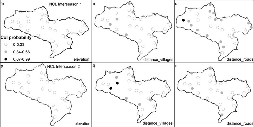
was by distance from villages during the Interseason 1 (Figure 5j–l). Distances from roads markedly    distance    from  roads
   more than
affected          it was by distance
           its colonization     compared  fromto villages
                                                 the effect during   the Interseason
                                                              of elevation               1 (Figure 15j–l).
                                                                             in the Interseason              Distances
                                                                                                       (Figure     5m–o).from
                                                                                                                            In the
   roads   markedly      affected  its  colonization    compared      to the  effect  of elevation
Interseason 2, distance from villages had a greater influence than elevation and distance from roads  in  the  Interseason     1
   (Figure   5m–o).
(Figure 5p–r).         In the Interseason    2, distance   from  villages   had a greater   influence   than   elevation   and
   distance from roads (Figure 5p–r).

                                                        Figure 5. Cont.

  Animals 2020, 10, x; doi: FOR PEER REVIEW                                                  www.mdpi.com/journal/animals
Animals 2020, 10, 1333                                                                                                         13 of 20
  Animals 2020, 10, x FOR PEER REVIEW                                                                                       2 of 20

         Figure
      Figure    5. 5.Differences
                      Differences between
                                   between effects
                                              effects of
                                                      of elevation
                                                         elevation and
                                                                     anddistance
                                                                          distancefromfromvillages
                                                                                              villagesandand roads
                                                                                                               roads onon
                                                                                                                        local
                                                                                                                           local
         colonization    and  extirpation of LC   and  NCL  in the TNR,   (a)–(i) are maps    of the
      colonization and extirpation of LC and NCL in the TNR, (a–i) are maps of the leopard cat and    leopard    cat and (j)–
                                                                                                                            (j–r)
      are(r)maps
             are maps   for North
                   for the  the North  Chinese
                                   Chinese       leopard.
                                             leopard.     Proportionsin
                                                        Proportions    inlegend
                                                                          legend are
                                                                                   are applicable
                                                                                       applicabletotoall allmaps.
                                                                                                             maps. The same
                                                                                                                      The  same
         line
      line     representsvariables
            represents      variables in
                                      in the
                                         the same
                                              sameinterseason
                                                     interseasonforfor
                                                                     species on on
                                                                       species    thethe
                                                                                      left left
                                                                                            mapmapin the
                                                                                                       inline.
                                                                                                          the Col
                                                                                                                line.and
                                                                                                                       ColExt
                                                                                                                            and
         probability    mean,   respectively,  colonization  and  extirpation   probability    (each   dot
      Ext probability mean, respectively, colonization and extirpation probability (each dot on these maps  on  these  maps
         represents one sample site and only significant differences were mapped).
      represents     one sample site and only significant differences were mapped).

  3.3.
3.3.   Multi-YearAssessment
     Multi-Year   AssessmentofofSpecies
                                 SpeciesCo-Occurrence
                                        Co-Occurrence

      LCLC    showedpositive
          showed       positiveco-occurrence
                                 co-occurrence with
                                                  with RF
                                                       RF and
                                                            and independent
                                                                 independentcohabitation
                                                                                  cohabitation (φ(ϕ
                                                                                                  ~ 1~ everywhere;
                                                                                                        1 everywhere;
   Table
Table  6).6).
           It It hadcomparatively
               had    comparativelyhigher
                                       higher occupancy
                                               occupancy atat sites
                                                              siteswhere
                                                                     whereRF RFwas
                                                                                 wasdetected
                                                                                       detectedduring
                                                                                                 duringthethe
                                                                                                           first two
                                                                                                              first two
   sampling    periods.  RF colonization   and  extirpation probabilities   were  relatively higher in
sampling periods. RF colonization and extirpation probabilities were relatively higher in the presence the presence
of of
    LCLCduring
          duringboth
                   both interseasons
                         interseasons (gamAB
                                         (gamABand andgamAb;
                                                        gamAb;  Table  6). RF
                                                                   Table   6). had
                                                                                RF true
                                                                                    had co-occurrence   (φ > 1) (ϕ
                                                                                         true co-occurrence     with> 1)
   NCL in all seasons and comparatively higher occupancy at sites where NCL occurred only in season
with NCL in all seasons and comparatively higher occupancy at sites where NCL occurred only in
   one. NCL colonization was relatively higher in the absence of RF (gamAb; Table 6). LC tended to
season one. NCL colonization was relatively higher in the absence of RF (gamAb; Table 6). LC tended
   avoid NCL (φ < 1) during sampling period one and occurred independently of the other two
to avoid NCL (ϕ < 1) during sampling period one and occurred independently of the other two
   interseason (φ ~ 1). The LC occupancy was high in the absence of NCL in season one (psiBA; Table
interseason (ϕ ~ 1). The LC occupancy was high in the absence of NCL in season one (psiBA; Table 6).
   6). NCL colonization and extirpation were comparatively higher during Interseason 1 in the absence
NCL    colonization
   of LC  and duringand     extirpation
                        Interseason   2 in were  comparatively
                                           the presence  of LC. Allhigher   duringmodel
                                                                     coexistence     Interseason  1 in thedescribed
                                                                                           combinations     absence of
LCa and
     crescent-shaped φ over 3 years. The lowest φ was 0.93 ± 0.10 and the highest φ was 1.67 ± 0.18 for a
          during    Interseason   2 in the  presence  of  LC.  All  coexistence   model   combinations     described
crescent-shaped
   NCL-LC and NCL-RF,         3 years. The lowest ϕ was 0.93 ± 0.10 and the highest ϕ was 1.67 ± 0.18 for
                     ϕ over respectively.
NCL-LC and NCL-RF, respectively.

      Table 6. Dynamic co-occurrence results for NCL (Species A) and RF and LC (Species B), the probability
      of occupancy of RF and LC when leopard is present (psiBA) or absent (psiBa), including the leopard
      colonization and extirpation probabilities when RF and LC are present (gamAB/epsAB) or absent
      (gamAb/epsAb) during the interseason. The table contains also the species interaction factor (SIF)
      of species’ pair co-occurrence. Estimates are accompanied by standard errors and NA indicates not
      applicable because colonization and extirpation probability are present only in interseasons.

   Season         psiBA            psiBa           gamAB            gamAb             epsAB            epsAb               ϕ
                                                                RF-LC
     one        0.78 (0.08)      0.66(0.27)       0.22 (0.20)      0.20 (0.18)      0.29(0.10)       0.15(0.13)       1.01(0.05)
     two        0.81 (0.09)      0.69(0.16)       0.36 (0.12)      0.31 (0.28)      0.22(0.11)       0.19(0.22)       1.11(0.15)
    three       0.56 (0.11)      0.63(0.10)          NA               NA               NA               NA            1.20(0.10)
Animals 2020, 10, 1333                                                                                   14 of 20

                                                   Table 6. Cont.

   Season         psiBA         psiBa        gamAB         gamAb         epsAB        epsAb          ϕ
                                                      NCL-RF
      one       0.55 (0.11)   0.26 (0.15)   0.38 (0.24)   0.39 (0.24)   0.28(0.11)   0.17(0.18)   1.23(0.12)
      two       0.35 (0.12)   0.51(0.11)    0.45 (0.24)   0.47 (0.19)   0.19(0.12)   0.24(0.20)   1.65(0.19)
     three      0.62 (0.24)   0.68(0.12)       NA            NA            NA           NA        1.67(0.18)
                                                      NCL-LC
      one       0.77 (0.12)   0.82(0.10)    0.42 (0.21)   0.44 (0.47)   0.10(0.20)   0.13(0.20)   0.93(0.10)
      two       0.77 (0.15)   0.60(0.20)    0.45 (0.15)   0.39 (0.23)   0.29(0.18)   0.22(0.17)   1.06(0.16)
     three      0.63 (0.15)   0.46(0.17)       NA            NA            NA           NA        1.14(0.10)

4. Discussion

4.1. Species Estimates across Years
      We built generic models wherein variations were computed according to year and seasonal RF
and site-specific LC and NCL effects (Table 3). The model outputs indicated that species occupancy
did not markedly fluctuate over time. Species occupancy is useful for predicting species distribution,
providing relevant inferences [10,39,51]. The constancy of occupancy of NCL, RF, and LC in the
TNR demonstrated the stability of the factors that govern the dynamic process by which species
adjust to various landscape perturbations due to human activities. Sustainable management practices
(afforestation, compensation for livestock depredation, regular wildlife monitoring, etc.) form the basis
for this stability. The protected area of this study has benefited from recent Chinese government policies
under the Natural Forests Protection Program for landscape restoration and the improvement of
management strategies. These measures have increased the size and enhanced the value of the forests
and protected areas [52,53]. In the TNR landscape, the NCL is an umbrella species [3]. Its protection
will augment the survival of other carnivores such as RF and LC [5,23].
      MacKenzie [38] analyzed occupancy models with 40 sampling stations and proposed that site
occupancy estimates are usually unbiased at detectability >0.3. They recommended ≥5 sampling
occasions. We disclosed detection probabilities >0.3 during all sampling periods for RF and within
Sampling Periods 1 and 3 for LC and NCL. During Sampling Period 2, however, the detection
probabilities were 0.28 ± 0.03 and 0.24 ± 0.04 for LC and NCL, respectively. According to the number of
sampling sites, the dataset was adequate. Based on the conclusions of Nicholson and Van Manen [10]
(one season depicts a detectability
Animals 2020, 10, 1333                                                                              15 of 20

be 0.42 ± 0.10. Because the NCL occupancy was  1800 m.a.s.l. for a study in South
America [54] which contradict our findings about the NCL. Habitat structure and vegetation type
strongly determine occupancy of carnivore species [12,55].
      NCL preferred sites remote from human settlements (villages and roads). Carnivores, especially
large ones prefer high densities of vegetation cover [54], prey availability [14,23], and quiet, hidden
places [55]. Here, NCL colonization slightly increased at sites near villages. These areas are always in
contact with carnivores. Nevertheless, low human tolerance for the presence of felids might alter the
occupancy of these species in areas surrounding human settlements and threaten carnivore population
dynamics [31]. Colonization is a conditional occupancy [38]. Therefore, species adjust their behavior in
order to gain access to these sites instead of occupying the vicinity of villages [56,57]. Entry into these
areas might enable the animals to prey upon livestock herds. Seasonal livestock proliferation within a
part of the landscape during a sampling period might account for the renewed presence of a large
carnivore and could be perceived as colonization. These patterns are common to numerous protected
areas hosting both carnivores and livestock herders [16,55]. The villages seem to become a sink for the
NCL population, and carnivores are alternately attracted in their vicinity. The attraction is based on
the proliferation of easy catching prey which enhances human–carnivore interactions. Across years
such situation would have serious consequences on species population of NCL in this region since the
transformation of a proportion of leopard to sink population status will be permanent if nothing is
undertaken by reserve’s managers. However, RF reacted identically as NCL to human settlements.
This behavior may result in spatial overlap with NCL in sites remote from villages. The LC is closer
to villages in the TNR, and its occupancy increased as distance from villages increased. Therefore,
the LC interacts with villagers’ activities and can prey on poultry or small domestic mammals as
the species selects areas with prey that are easy to catch rather than those with high population
density [27]. An investigation carried out on LC–human interactions could validate this assumption
for TNR. This type of contact influences even small- or medium-size species distributions within a
landscape [16,58]. There are few published studies of anthropogenic pressure on small carnivores and
the effects and mechanisms involved are poorly understood [31,59–61].
      In contrast, variable effects on the local species extirpation probabilities were lower than those
for colonization. Hence, the variables had different effects. Human presence remains a potential
You can also read