Agriculture, Ecosystems and Environment - Thünen-Institut: Literaturrecherche
←
→
Page content transcription
If your browser does not render page correctly, please read the page content below
Agriculture, Ecosystems and Environment 322 (2021) 107640
Contents lists available at ScienceDirect
Agriculture, Ecosystems and Environment
journal homepage: www.elsevier.com/locate/agee
New N2O emission factors for crop residues and fertiliser inputs to
agricultural soils in Germany
Gokul Prasad Mathivanan a, Max Eysholdt b, Maximilian Zinnbauer b, Claus Rösemann a,
Roland Fuß a, *
a
Thünen Institute of Climate-Smart Agriculture, Braunschweig, Germany
b
Thünen Institute of Rural Studies, Braunschweig, Germany
A R T I C L E I N F O A B S T R A C T
Keywords: Direct agricultural N2O emissions in Germany have so far been estimated using the default Tier 1 emission factor
N2O emissions of 1% (0.3–3%) in accordance with the IPCC’s default methodology. Since direct N2O emissions is a “key
Greenhouse gas inventory category” in the German National Greenhouse Gas Inventory, the IPCC recommends the use of country-specific
Emission factors
emission factors or models. With the aim of deriving country-specific and stratified N2O emission factors, a meta-
Fertilisation
analysis was conducted using data collected from 71 individual studies comprising 676 separate emission
measurements taken at 43 locations across Germany. A Bayesian generalised linear mixed-effects modelling
approach was used to model N2O fluxes and derive emission factors. In contrast to what is suggested by the 2019
Refinement to the 2006 IPCC Guidelines, the model results did not support a distinction being made between
emission factors for synthetic and organic fertilisers. Instead, a model based on four environmental zones roughly
representing the north-west, north-east, south-east and south-west parts of the country was developed. It was
used to derive district-wise emission factors for direct N2O emissions and revealed that northern districts had
relatively lower emission factors than southern districts. The district-wise emission factors ranged from 0.38% to
0.92%. The national implied emission factor for direct N2O emissions from managed agricultural soils was 0.62%
(0.43–0.85%). Accordingly, the estimate of German national GHG emissions from agriculture in 2015 is 8.59%
(calculated with global warming potentials from IPCC’s fifth assessment report) lower than the estimate reported
in the 2021 inventory submission to UNFCCC.
1. Introduction secretariat. Germany is one such country.
The Intergovernmental Panel on Climate Change (IPCC) provides
Nitrous oxide (N2O) is a strong greenhouse gas and catalyses the guidelines for countries to estimate N2O emissions along with other
depletion of ozone in the stratosphere (IPCC, 2014a; Ravishankara et al., GHGs for reporting in their national inventories. The guidelines provide
2009). It is the third strongest contributor to global warming after car three “Tiers” based on the depth of data and scientific knowledge
bon dioxide (CO2) and methane (CH4) (WMO, 2021). With an atmo available to estimate emissions. Tier 1 uses global default emission
spheric lifetime of 131 years, it has a global warming potential (GWP) factors (EFs), Tier 2 uses stratified or country-specific EFs, and Tier 3
265 times that of CO2 over a 100-year time horizon (IPCC, 2014a). uses measurements or complex modelling approaches requiring process-
Approximately 40% of global N2O emissions have anthropogenic sour specific data at high resolutions (IPCC, 2006). An EF expresses the
ces with more than half of these being direct emissions from fertiliser emission released by a specific and standard quantity of activity or
nitrogen (N) inputs in agriculture (Tian et al., 2020; WMO, 2021). input. In the case of direct N2O emissions from N inputs to agricultural
As the basis of efforts to limit global warming (COP, 2015), accurate soils, the emission factor is the proportion of N input emitted as N2O.
inventories of anthropogenic GHG emissions are essential. Signatories to Tier 1 (the lowest tier) uses a default emission factor (1% of N input)
the United Nations Framework Convention on Climate Change (United derived from global N2O measurements (IPCC, 2019, 2006). The pro
Nations, 1992) and in particular countries listed as Annex I parties gression from lower to higher tiers increases the accuracy and also often
therefore submit national emission inventories annually to the UNFCCC reduces the uncertainty in estimating N2O emissions and is therefore
* Corresponding author.
E-mail address: roland.fuss@thuenen.de (R. Fuß).
https://doi.org/10.1016/j.agee.2021.107640
Received 29 July 2021; Received in revised form 24 August 2021; Accepted 24 August 2021
0167-8809/© 2021 The Author(s). Published by Elsevier B.V. This is an open access article under the CC BY license (http://creativecommons.org/licenses/by/4.0/).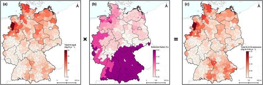
G.P. Mathivanan et al. Agriculture, Ecosystems and Environment 322 (2021) 107640
recommended by the IPCC guidelines. (Butterbach-Bahl et al., 2013). Due to the complex interaction of mi
The default Tier 1 EF for direct N2O emissions from N inputs to soils crobial processes, many factors are known to have an impact on N2O
(EF1) has evolved over the years. The IPCC’s revised 1996 guidelines emissions. These include substrate nitrogen species, soil pH, soil organic
(IPCC, 1997) had estimated an emission factor of 1.25% (0.25–2.25%) carbon (SOC), soil texture, soil moisture and temperature, and
but related this value to the N input remaining in soil after ammonia freeze-thawing events (Liu et al., 2010; Risk et al., 2013). Various
volatilisation and nitric oxide emissions. With new N2O measurement drivers of N2O emissions have been identified in different countries. The
studies and data becoming available, the 2006 IPCC guidelines (IPCC, United Kingdom, for example, has identified fertiliser type (urea-based
2006) modified EF1 to 1% (0.3–3%) of N input without deducting and other fertilisers) and annual rainfall to be primary drivers of N2O
ammonia and nitric oxide losses. In 2019, the IPCC reduced the uncer emission whereas moisture regimes and topographic conditions are
tainty range of EF1 to 0.1–1.8% and published a disaggregated Tier 1 among the influential factors in Canada (Brown et al., 2021; Environ
approach that stratifies by climate (“wet” and “dry”) and within wet ment and Climate Change Canada, 2021). Previous meta-analyses of
climates between synthetic fertilisers and other, i.e. organic or mixed N N2O emissions in Germany have given preliminary knowledge about the
inputs (IPCC, 2019). This disaggregated Tier 1 approach increases EF1 magnitude and variability of N2O emissions and about the main factors
for synthetic fertilisers to 1.6% (1.3–1.9%) and decreases it for other N influencing them. Dechow and Freibauer (2011) identified climate and
inputs to 0.6% (0.1–1.1%). soil properties to be key influencers of N2O emissions and found the
Germany is the second largest contributor of direct N2O emissions average emission factor for N2O emissions from mineral soils to be about
from managed agricultural soils in Europe. For 2019, Germany reported 0.9%. Jungkunst et al. (2006) estimated a mean emission factor of
direct N2O emissions of 67.29 kt N2O, which is 14.8% of Europe’s N2O 1.56% (median 0.63%), with the emission factor significantly varying
emissions and is only surpassed by France’s contribution of 19.1% according to the country’s climatic zones.
(European Environment Agency, 2021). The direct N2O emissions from The objective of this study was to develop a new Tier 2 methodology
agricultural soils in 2019 are 71.21% of the total N2O emissions from to estimate German N2O emissions associated with N input based on a
German agriculture, which include N2O emissions from livestock meta-analysis of scientific results on N2O emissions from agricultural
farming and manure management as well as indirect N2O emissions soils. The meta-analysis was designed to identify the major factors
from nitrate leaching and N volatilisation. N2O emissions from agri influencing N2O emissions in Germany and thereby provide a robust
cultural soils are classified as a “key category” in the German national basis for determining country-specific Tier 2 emission factors. Particular
greenhouse gas inventory due to their significant contribution to overall attention was given to ensuring the methodology was in line with IPCC
emissions and the emission trend over time (Federal Environment guidelines and tailoring the approach so that it could be part of the
Agency, 2021). Despite being part of a key category and the IPCC preparation of Germany’s national greenhouse gas inventory.
guidelines recommending the use of a higher tier approach for key
categories, direct N2O emissions in Germany are still being estimated 2. Materials & methods
using the default Tier 1 EF. While it may be suitable for estimating
emissions at a global level, the Tier 1 approach does not accurately 2.1. Data collection and organisation
represent the actual direct N2O emissions for many countries. Top-down
estimates of N2O emissions derived from inverse modelling based on Data collection started with the N2O measurement data used in the
atmospheric gas concentrations are not in good agreement with 2019 Refinement to the 2006 IPCC Guidelines for National Greenhouse
bottom-up estimates derived from inventory approaches at regional and Gas Inventories consisting of 332 studies, of which 23 were from Ger
sub-regional levels (Shcherbak et al., 2014; Tian et al., 2020). While many. A literature review of N2O measurement studies conducted in
there is good agreement at the global level and some regions such as Germany was undertaken to increase the number of studies and expand
South and South-East Asia, the top-down estimates are substantially the total number of measurements. A “measurement” hereinafter refers
lower than the bottom-up estimates for Europe (Tian et al., 2020), which to the mean of all replicate N2O measurements belonging to a treatment
could indicate an overestimation due to the Tier 1 EF1 being too high for in a study. The scientific literature databases Web of Science and Google
Europe. This disagreement therefore emphasises the need to derive Scholar were searched for peer-reviewed literature using keywords ‘N2O′
country-specific Tier 2 EFs and investigate the appropriateness of the and ‘Germany’. Apart from the exclusion criteria adopted in the IPCC’s
default Tier 1 EF for estimating country level N2O emissions of European original database, such as the exclusion of studies conducted in the
countries such as Germany. laboratory, organic soils, grazing studies, modelling studies and studies
Country-specific emission factors can only be derived when there is involving slow-release or inhibitor-stabilised fertilisers, three further
adequate availability of N2O measurement data and sufficient stratified exclusion criteria were included: studies pertaining to natural N2O
activity data, and are therefore difficult for many countries to achieve. sources, studies whose measurement period was less than 150 days, and
As of 2021, only nine of the 43 UNFCCC Annex I countries have adopted measurements that were taken from fallow land and legumes. Mea
Tier 2 or Tier 3 approaches to estimate N2O emissions (UNFCCC, 2021). surements with legumes were excluded because the additional N input
However, numerous N2O measurement studies have been conducted from N fixation could generally not be quantified with the available
over the past three decades throughout Germany, making it feasible to data. Unlike the IPCC database, studies conducted on organic soils were
derive a national emission factor for the country. included in the data collection.
The Tier 2 method requires stratified emission factors corresponding In order to have a sufficient number of measurements in each loca
to variables influencing N2O emissions. N2O emissions from agricultural tion and make the modelling process more robust, measurement loca
soils result primarily from microbial processes in the nitrogen cycle. tions close to each other were grouped together to form location clusters.
Under aerobic conditions, ammonia is oxidised to nitrate via the in In view of the different emission dynamics between mineral and organic
termediates hydroxylamine and nitrite, with N2O produced as a by- soils, the database was split into two different data sets for mineral and
product during hydroxylamine oxidation (Wrage et al., 2001). Even organic soils. Following the German national greenhouse gas inventory
more important for N2O emissions is the anaerobic process of denitri definition (Federal Environment Agency, 2021), locations with SOC
fication, which is the reduction of nitrate to N2. Since N2O is an inter content greater than 9% were classified as organic soils and the rest
mediate of this process and many microorganisms, in particular fungi, categorised as mineral soils. This national threshold is slightly lower
do not produce N2O reductase, large quantities of N2O can be emitted as than the IPCC default threshold of 12% (IPCC, 2014b).
a result of incomplete denitrification (Wrage et al., 2001). While nitri Because cumulated emissions can be expected to correlate with
fication and denitrification are the dominant N2O forming processes, measurement period, the measurement period was included in the
other microbial and chemical processes can be of relevance locally database as a separate ‘short-by’ variable. By including this variable in
2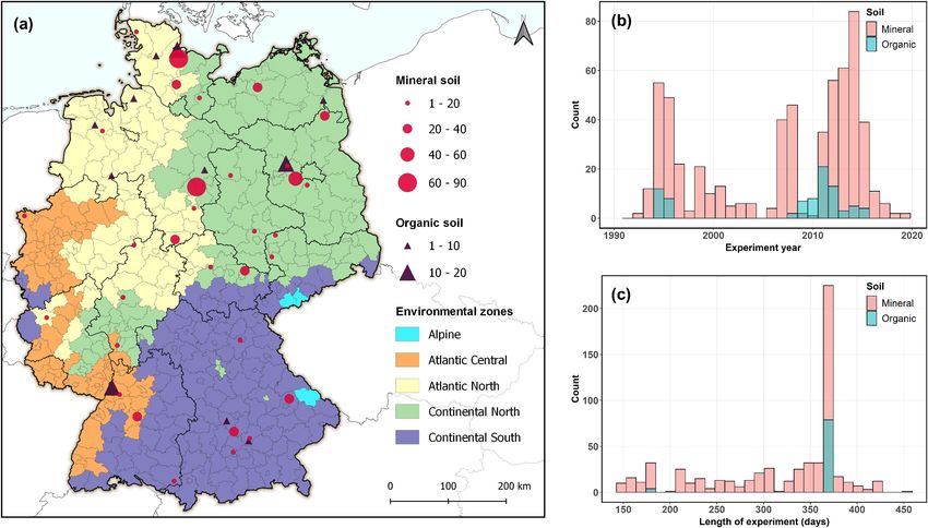
G.P. Mathivanan et al. Agriculture, Ecosystems and Environment 322 (2021) 107640
the models, it is possible to account for the confounding effect of mea For each model, the root mean squared error of the model fit
surement period and the transformation (short-by = 365 d – measure (RMSEfit) showing goodness of fit was calculated. In addition, the pre
ment period) allows extracting annual emission factors directly from the dictive performances of the models were evaluated using a k-fold cross-
model fit. validation approach (with folds corresponding to location clusters)
Weather data from Germany’s national meteorological service which resulted in the root mean squared error of cross-validation
(DWD) were used to calculate long-term annual average precipitation (RMSEcv). Besides the root mean squared error of the model fit and
and temperature (1990–2019) for studies lacking this information. Data cross-validation, a PSIS-LOO (Pareto smoothed importance sampling
from the German agricultural soil inventory (BZE-LW) were used to fill leave-one-out; Vehtari et al., 2017) cross-validation was also performed
in missing SOC and pH values. Soil parameters for the depth 0–30 cm on the models to give a LOO information criterion (LOOIC) estimate.
were included in the database and calculated from more detailed data While the LOOIC values do not have any intrinsic meaning for individual
where necessary. Locations were categorised according to their envi models, they allow the models’ performance to be compared.
ronmental conditions, using the environmental stratification zones from
Metzger et al. (2005). A few of these zones were merged to ensure each
of them contained a sufficient number of data points for modelling 2.3. Derivation and application of emission factors
(Fig. 1a). There is no agricultural land use in the Alpine zone.
The N2O EFs for mineral and organic soils were averaged for each
2.2. Modelling methods district (NUTS level 3 region; European Community, 2003), based on
their respective agricultural area, to derive a unified N2O EF for each
Modelling was performed separately for mineral and organic soils. district. The agricultural area (which includes cropland and grassland)
The modelling approach followed that of Bouwman (1996) who of organic and mineral soils was taken from the database of the German
modelled N2O emissions as a linear function of N application rates, LULUCF inventory (Federal Environment Agency, 2021).
making EF the slope of this model. The advantage of such a linear model The regional (district-wise) distribution of organic fertilisers and N
is that it ensures that using the sum of N inputs to soil as the model input inputs, i.e. biogas digestates, sewage sludge, manure and crop residues,
results in the sum of emissions, i.e. Σf(x) = f(Σx), which is not the case was taken from the database of the German agricultural GHG inventory
for non-linear models. N2O emissions generally exhibit a positively (Rösemann et al., 2021). Regional data on synthetic fertiliser applica
skewed pattern, with extreme values towards the higher tail. Previous tions are not available in Germany. There are statistics on synthetic
studies, such as Stehfest and Bouwman (2006) and Walter et al. (2015), fertiliser sales for NUTS level 2 regions, but due to interregional fertiliser
have handled this by log-transforming N2O emissions, which, after trading these do not represent actual synthetic fertiliser use. Therefore,
back-transformation results in an exponential model. However, in the data on the regional distribution of synthetic fertiliser input for the
present study, N2O emissions were not transformed, in order to preserve period 2014–2016 were derived from regional agricultural nitrogen
linearity. Instead, a generalised linear mixed model (GLMM) with the balances, which were modelled at municipality level. The Regional
gamma distribution family and an identity link function was used to Agricultural and Environmental Information System (RAUMIS) was
account for the skewness. A gamma distribution can approach varying used as the model framework. RAUMIS is a regional agricultural supply
levels of skewness (from symmetric to heavily skewed) depending on its model that depicts agricultural production and income at district level
shape parameter, which is estimated during model fitting. The (NUTS level 3), ensuring consistency with regional and sectoral statis
mixed-effects model approach was used to account for correlation tical information (Gömann et al., 2002; Henrichsmeyer et al., 1996). The
within location clusters and within the measurement years by including model encompasses a series of environmental indicators such as spatial
these as random effects. nutrient balances, that have been previously applied in nitrogen-related
The model fitting process was undertaken using the Bayesian policy analyses in several studies (Ackermann et al., 2016; Henseler and
approach. This allows prior knowledge about model parameters to be Dechow, 2014; Kreins et al., 2007).
fed into the model as a prior probability distribution (‘prior’) which is Municipality-level agricultural nitrogen flows were modelled using
then updated using the available data and results in a posterior proba municipality-level statistical land use and livestock data from the Thü
bility distribution (‘posterior’). Another advantage of this modelling nen Agraratlas,1 regional yields, spatially explicit data on biogas plants,
method is that convergence can be difficult to achieve with complex and data on inter-regional manure transportation as the core database.
generalised linear mixed-effects models and the underlying Markov Nitrogen uptake from grazing and grassland management was modelled
chain Monte Carlo (MCMC) sampling algorithm of the Bayesian model by a simplified balance of demand and supply of roughage as a feedstock
helps avoid such difficulties by sampling over many chains, thereby to livestock and biogas plants.
increasing the likelihood of a successful fit. The Bayesian models were Regional synthetic fertilisation was derived using linear, yield-
run in the R statistical computing platform (version 4.0.5, R Core Team, depending nutrient requirement functions (Kreins et al., 2010).
2021) using the ‘rstanarm’ package (version 2.21.1 (Goodrich et al., Site-specific characteristics affecting synthetic fertiliser requirements
2020; Stan Development Team, 2020)). were included by deriving a local site factor (Henrichsmeyer et al., 1996;
Several models were constituted with a combination of potential Krüll, 1988). RAUMIS calculates synthetic fertiliser inputs (S) as
predictors based on similar N2O emission factor studies in Germany and
Sm = β * Rm – α * Om,
other countries. ‘Location’ and ‘measurement year’ remained as random
effects in all the models. The priors assigned to the fixed effects were where m indicates the municipality, β is a global adjustment factor, R is
primarily based on the 2019 refinement to the IPCC guidelines, where the aggregated crop-specific and site-specific nitrogen requirement
available, or otherwise on our own expert judgement. derived from harvest data taking the preceding crop and nitrogen fixa
Based on the availability of sufficient and necessary activity data, tion into consideration, and O is the total amount of organic nitrogen
two types of models were formulated for the mineral soil subset: applied (Henrichsmeyer et al., 1996). Only a part of this organic nitro
inventory-specific models that are in line with IPCC guidelines and are gen is available for the crop. This available proportion α and the factor β
suitable for available national data, and a field-level model where the were calibrated in such a way that aggregated regional fertiliser inputs
availability of activity data is not a constraint. A further separate model
was formulated for the organic soil data subset to derive a separate N2O
EF for organic soils. An overview of the various generalised linear 1
Processed data. Original data from Statistische Ämter des Bundes und der
mixed-effects models derived for mineral and organic soils is given in Länder (2018) derived with the method from Gocht and Röder (2014). Version
Table 1. 2020.
3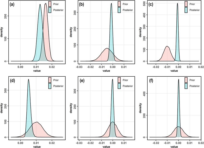
G.P. Mathivanan et al. Agriculture, Ecosystems and Environment 322 (2021) 107640
Fig. 1. (a) Map of Germany showing the five environmental zones and the location clusters of measurements. Symbol size indicates the number of measurements.
Borders of federal states and districts are indicated. (b) Number of data points per year. (c) Histogram showing the measurement period.
equalled the averaged national statistics on synthetic nitrogen fertiliser 3. Results
sales (Statistisches Bundesamt, 2016) for the observed time period. The
model ensures that the amount of mineral fertiliser applied is at least 3.1. N2O data
10% of the nitrogen amount required, in every region. This model
parameter, determined by experts from agricultural authorities based on Of the 71 studies (676 measurements) in the database, most of the
documentation of previously mandatory farm-level “nutrient compari N2O measurements had been performed on mineral soils (59 studies;
sons” (Gömann et al., 2020), reflects the minimum amount of mineral 593 measurements). Although N2O measurements on mineral soils had
fertiliser assumed to be necessary for an effective crop management. been taken throughout the country in 32 location clusters, about 75% of
Other model parameters (e.g. nitrogen contents of crops, nitrogen these measurements were from northern Germany in the Atlantic North
excretion per animal, share of crop residuals) were taken from (KTBL, and Continental North environmental zones (Fig. 1a). The measure
2018) and the German Fertilizer Ordinance (Düngeverordnung, 2021). ments were taken over a wide temporal range between 1992 and 2019
The model does not allow for a distinction between different types of (Fig. 1b), with most of the studies having measurement periods of more
synthetic nitrogen fertiliser. than 300 days (Fig. 1c). 22% of the measurements were from unfertilised
District-wise N inputs that were consistent with the emission in control treatments and 63% of studies included such a control treat
ventory were derived by dividing the modelled synthetic fertiliser use in ment. The pH of mineral soils ranged from 4.7 to 7.7 with a mean of 6.3
each district for the years 2014–16 by the modelled national total, and and the soil organic carbon (SOC) content was in the range of 0.5–4.7%
multiplying the resulting values by the total N input taken from the with a mean of 1.57%.
national GHG inventory for the year 2015. The district-wise sum of N In addition to grasslands (16% of measurements), prominent crops
inputs (synthetic fertilisers, animal manure, sewage sludge, biogas grown during the measurement period were winter wheat/barley (22%
digestate and crop residue) were then multiplied by the corresponding of measurements), winter oilseed rape (15% of measurements) and
district level unified EFs to derive total N2O emissions for each district maize (21% of measurements). Where measurements involved fertil
and thereby the whole country. The implied emission factors (IEF) for isation, most of the nitrogen fertilisation was done through ammonium
the individual and overall N inputs were calculated by dividing total nitrate fertilisers and the rest split almost equally between cattle
emissions by the appropriate national sum of each N source. Un manure, biogas digestate and a mixture of organic and synthetic fertil
certainties in N2O emission values were derived using the Monte Carlo isers. Ammonium nitrate fertilisers are the most common fertiliser
simulation based on Markov chain results from the model fit (i.e., Model category used in Germany. In 2015, the share of calcium ammonium
4 in Table 1). This approach only takes the uncertainty of the emission nitrate (CAN) in total fertiliser nitrogen sales was 35.6% and that of urea
model into account and not the uncertainty of the spatial distribution of ammonium nitrate solution (UAN) was 9.5% (Statistisches Bundesamt,
N inputs. The GWPs from the fifth assessment report of the IPCC (IPCC, 2016).
2014a) were used to convert emission units from N2O and CH4 to CO2 Eighty-three N2O measurements from 12 studies were made on
equivalents. organic soils. Similar to the mineral soils, approximately 70% of these
measurements were taken in northern Germany, where most of the
organic soils are located. The measurements were conducted between
1994 and 2015 and most of them had a measurement period of 365 days
except for four measurements that covered 184 days. Soil pH in the 11
4
Table 1
1 1
Linear mixed-effects models tested for direct N2O-N emissions. Posterior means for the intercept and slope are in units of kg N2O-N ha− yr − and kg N2O-N/ kg N applied respectively. Some illustrative plots of the model
components (priors and posteriors) can be found in the supplement.
Model Linear predictor Random effects Parameters Priors Posterior RMSEfit LOOIC RMSECV
No. (fixed effects) (normal distribution mean (kg N2O-N (kg N2O-N
On On slope
with (mean, S.D.)) (credible ha¡1 yr¡1) ha¡1 yr¡1)
G.P. Mathivanan et al.
intercept
interval)
Mineral soils
1 β0 + β1 • X1 + β2 • X2 by location, N input by β0: Intercept (emission at zero N(1,0.5) 1.62 (1.11, 2.16 1799 2.85
by year location fertiliser input) 2.19)
β1: Slope vs N input (emission N(0.01,0.0041) 0.0054
factor) (0.0035,
0.0079)
β2: Slope vs Experiment length N(0,1) − 0.0022
("short-by") (− 0.0045,
0.0001)
2 β0 + [β10 + β11 • (X2 == “mixed fertiliser”) + β12 • (X2 == “organic by location, N input by β0: Intercept (emission at zero N(1,0.5) 1.80 (1.26, 2.10 1808 3.25
fertiliser”)] • X1 + β2 • X3 by year location fertiliser input - synthetic fertiliser) 2.43)
β10: Slope vs N input (emission N(0.016,0.0015) 0.0125
factor - synthetic fertiliser) (0.0094,
0.0156)
β11: Slope vs N input (difference N(0.011,0.0051) − 0.0013
between synthetic and mixed (− 0.0035,
fertiliser) 0.0009)
β12: Slope vs N input (difference N(0.006,0.0025) − 0.0009
between synthetic and organic (− 0.0025,
fertiliser) 0.0006)
β2: Slope vs Experiment length N(0,1) − 0.0018
5
("short-by") (− 0.0041,
0.0004)
3 β0 + [β10 + β11 • (X2 == “mixed fertiliser”) + β12 • (X2 == “organic by location, N input by β0: Intercept (emission at zero N(1,0.5) 1.62 (1.12, 2.16 1804 2.85
fertiliser”)] • X1 + β2 • X3 by year location fertiliser input - synthetic fertiliser) 2.18)
β10: Slope vs N input (emission N(0.01,0.0041) 0.0055
factor - synthetic fertiliser) (0.0035,
0.0080)
β11: Slope vs N input (difference N(0,0.0041) − 0.0003
between synthetic and mixed (− 0.0023,
fertiliser) 0.0019)
β12: Slope vs N input (difference N(0,0.0041) 0.0002
between synthetic and organic (− 0.0013,
fertiliser) 0.0017)
β2: Slope vs Experiment length N(0,1) − 0.0022
("short-by") (− 0.0045,
0.0001)
4 [β00 + β01 • (X2 == “Atlantic North”) + β02 • (X2 == “Continental by location, N input by β00: Intercept (emission at zero N(1,0.5) 1.78 (1.11, 2.16 1800 2.78
North”) + β03• (X2 == “Continental South”)] + [β10 + β11 • (X2 == by year location fertiliser input - Atlantic Central) 2.49)
“Atlantic North”) + β12 • (X2 == “Continental North”) + β13• (X2 == β01: Intercept (difference between N(0,0.5) − 0.36 (− 1.08,
“Continental South”)] • X1 + β2 • X3 Atlantic Central and Atlantic 0.37)
North)
β02: Intercept (difference between N(0,0.5) − 0.35 (− 1.04
Atlantic Central and Continental to 0.34)
North)
β03: Intercept (difference between N(0,0.5) 0.24 (− 0.53,
Atlantic Central and Continental 1.01)
South)
β10: Slope vs N input (emission N(0.01,0.0041)
factor - Atlantic Central)
(continued on next page)
Agriculture, Ecosystems and Environment 322 (2021) 107640
Table 1 (continued )
     Model      Linear predictor                                                       Random effects              Parameters                             Priors                 Posterior         RMSEfit      LOOIC      RMSECV
     No.        (fixed effects)                                                                                                                           (normal distribution   mean              (kg N2O-N               (kg N2O-N
                                                                                       On             On slope
                                                                                                                                                          with (mean, S.D.))     (credible         ha¡1 yr¡1)              ha¡1 yr¡1)
                                                                                       intercept
                                                                                                                                                                                 interval)

                                                                                                                                                                                 0.0072
                                                                                                                                                                                                                                           G.P. Mathivanan et al.

                                                                                                                                                                                 (0.0037,
                                                                                                                                                                                 0.0108)
                                                                                                                   β11: Slope vs N input (difference      N(0,0.0041)            − 0.0023
                                                                                                                   between Atlantic Central &                                    (− 0.0061,
                                                                                                                   Atlantic North)                                               0.0017)
                                                                                                                   β12: Slope vs N input (difference      N(0,0.0041)            − 0.0033
                                                                                                                   between Atlantic Central &                                    (− 0.0071,
                                                                                                                   Continental North)                                            0.0006)
                                                                                                                   β13: Slope vs N input (difference      N(0,0.0041)            0.0017
                                                                                                                   between Atlantic Central &                                    (− 0.0036,
                                                                                                                   Continental South)                                            0.0071)
                                                                                                                   β2: Slope vs Experiment length         N(0,1)                 − 0.0021
                                                                                                                   ("short-by")                                                  (− 0.0044,
                                                                                                                                                                                 0.0003)
     5          [β00 + β01 • (X2 == “Atlantic North”) + β02 • (X2 == “Continental      by location,   N input by   β00: Intercept (emission at zero       N(1,0.5)               1.26 (0.57,       2.03         1712       2.71
                North”) + β03• (X2 == “Continental South”) + β04 • (X3 ==              by year        location     fertiliser input - Atlantic Central;                          1.96)
                “grassland”) + β05 • (X3 == “other crops”) + β06 • (X4 == SOC 1; pH >6; clay/
                + β07 • (X5 == pH 1 and SOC 6 and pH
G.P. Mathivanan et al. Agriculture, Ecosystems and Environment 322 (2021) 107640
organic soil location clusters was in the range of 3.3–7.2 (mean 5.4) and
ha¡1 yr¡1) SOC was in the range of 9.3–51.7% (mean 24.6%). Most of the N2O
(kg N2O-N
RMSECV
measurements were taken on grasslands (82% of measurements) and a
few on maize cropped lands (13% of measurements). Of these 83 mea
–
surements, 35 were taken under zero fertilisation conditions (83% of
studies included such a control treatment) while the remainder involved
LOOIC
402
ammonium nitrate fertilisers and cattle manure.
3.2. N2O emission models for mineral soils
ha¡1 yr¡1)
(kg N2O-N
RMSEfit
The IPCC Tier 1 method expresses N2O emissions only as a function
6.45
of N input. A corresponding model, only taking N inputs and the short-by
parameter into account (Model 1; Table 1), yielded an emission factor of
0.54% (0.35–0.79%). The negative coefficient of the short-by parameter
4.58 (2.13,
(− 0.0009,
(− 0.0056,
(− 0.0286,
Posterior
confirmed the expectation that cumulated N2O emissions in measure
(credible
− 0.0018)
interval)
− 0.0037
− 0.0111
(0.0011,
(0.0039,
0.0044)
0.0055)
0.0165)
0.0026)
0.0017
0.0033
0.0101
ments conducted for more than a year are higher, while shorter mea
mean
7.45)
surement periods correspond with lower emissions. The random
intercepts grouped by measurement year appeared to be completely
(normal distribution
random which suggests the absence of a temporal trend that might be
with (mean, S.D.))
expected due to developments in measurement methodology or due to
N(0.01,0.0041)
N(7.85,16.8)
climate change. In Model 2 (Table 1), N input was then stratified by
N(0,0.0041)
fertiliser type, i.e. synthetic and organic fertilisers as suggested in the
N(0,1)
N(0,1)
Priors
IPCC (2019) refinement’s disaggregated Tier 1 approach. Fertilisation
for measurements that included both synthetic and organic fertilisers
were categorised as mixed N inputs. The stratified EFs proposed by the
2019 refinement were taken as priors for synthetic fertilisers (1.6%) and
β14: Slope vs N input (difference
β15: Slope vs N input (difference
β2: Slope vs Experiment length
β2: Slope vs Experiment length
β0: Intercept (emission at zero
β1: Slope vs N input (emission
organic (0.6%) N inputs. For mixed N inputs, the mean of the two EFs
winter crops & other crops)
winter crops & grassland)
(1.1%) was used. The model contained the EF of synthetic fertilisers and
the differences between EFs of other N inputs and synthetic fertilisers as
slope parameters. The posterior emission factor for synthetic fertilisers
fertiliser input)
was 1.25% (0.99–1.51%) and the emission factors for mixed and organic
Parameters
("short-by")
("short-by")
fertilisers were 1.12% (0.81–1.44%) and 1.16% (0.87–1.45%), respec
Organic soils
tively (Fig. 2, which shows the difference between EFs). Differences in
factor)
EF between fertilisers were barely significant and the EFs were much
higher than the overall EF derived from Model 1. This can be attributed
to the high EF with narrow uncertainties, which was used as the prior for
N input by
On slope
location
synthetic fertilisers, thus allowing only extremely small probabilities of
a low EF.
Random effects
The same model was fit with neutral priors, i.e. EF = 1% for syn
thetic, mixed and organic fertilisers. The neutral priors were chosen in
by location,
intercept
such a way that they assign non-zero probabilities to the 2019 refine
by year
ment result. Using the neutral priors resulted in a very different fit
On
(Model 3; Table 1). The emission factor of synthetic fertilisers (0.55%;
0.37–0.75%) was almost the same as that of the EF from Model 1.
Similar to Model 2 with strong priors for fertilisation, the emission
factors for mixed (0.52%; 0.29–0.77%) and organic (0.56%;
0.37–0.78%) fertilisers were practically identical to that of synthetic
fertiliser (Fig. 2). Both models involving fertiliser types did not have
better performance metrics than the basic model, which indicates that
the type of fertiliser had practically no impact on N2O emissions.
Environmental zones, however, did have a strong effect on N2O
emissions (Model 4; Table 1). N input had the default 1% EF as prior and
neutral priors were used for the differences in EF between the envi
ronmental zones. The EFs of the environmental zones were clearly
distinguishable from a geographic perspective. Continental South had
the highest EF (0.88%, 0.38–1.43%) followed by Atlantic Central
(0.72%, 0.37–1.08%), Atlantic North (0.49%, 0.26–0.78%) and Conti
β0 + β1 • X1 + β2 • X2
nental North (0.39%, 0.17–0.66%). Thus, a clear divide was seen be
Linear predictor
tween the EFs of the environmental zones in northern and southern
(fixed effects)
Germany. While having a slightly higher LOOIC value than the base
Table 1 (continued )
model, the model with environmental zones had an identical RMSE of
model fit and a marginally better predictive performance RMSE. Thus,
although the performance was similar to Model 1, this model was
preferable because it allowed the geographic distribution of N input to
Model
be taken into account, thereby increasing the accuracy of estimations of
No.
6
total national emissions.
7G.P. Mathivanan et al. Agriculture, Ecosystems and Environment 322 (2021) 107640
Fig. 2. Comparison of prior vs posterior distributions of Model 2 (a,b,c) with strong priors for fertiliser types and Model 3 (d,e,f) with neutral priors. Distributions in
a and d represent the emission factor for synthetic fertilisers; b and e represent the difference between emission factors of synthetic and mixed fertilisers; c and f
represent the difference between emission factors of synthetic and organic fertilisers.
A more complex model included the variables crop categories, SOC, modelled separately since the factors influencing N2O emission in these
pH and texture in addition to environmental zones (Model 5; Table 1). soils were expected to be different from those of mineral soils, e.g.
The crop types were consolidated and categorised as ‘winter crops’, groundwater levels have a strong impact and strong mineralisation of
‘grassland’ and ‘other crops’. Clay and silt texture classes were grouped soil organic matter occurs in drained organic soils. Since the number of
together to form 3 texture classes: ‘sand’, ‘loam’ and ‘clay/silt’. SOC and N2O measurements was too small to explore the influence of possible
pH were grouped into two discrete classes, [1] and [6] predictors, a simple mixed-effects model was formulated using N input
respectively, so that measurements were split uniformly in each class. and short-by with location clusters and experiment year as random ef
This model, whose predictors were similar to that of Stehfest and fects (Model 6; Table 1).
Bouwman (2006) except for fertiliser types, performed marginally better Following the guidance of IPCC (2014b), the default emission factor
than all the other models. The EFs for winter crops in this model were of 1% (0.1–1.8%) from the IPCC (2019) was also used as the prior for N
similar to those of Model 4 whereas the EFs for grasslands and other input to organic soils and a neutral prior was given for the short-by
crops were higher in magnitude. parameter. The prior for emissions at zero fertilisation was derived
Emissions at zero fertilisation were consistently higher than the from the German Tier 2 methodology for estimation of N2O emissions
assigned prior of 1 kg N2O-N ha− 1 yr− 1 in all the models except for the resulting from mineralisation of soil organic matter in drained organic
complex model 5, which had emission at zero fertilisation lower than the soils (Tiemeyer et al., 2020). The mean of the emission factors for
assigned prior in the Atlantic North environmental zone (0.81 kg N2O-N cropland and grassland in drained organic soils was used as the prior, i.
ha− 1 yr− 1). They were in a similar pattern to that of the EFs for the four e., the expected value of the prior was 7.9 kg N2O-N ha− 1 yr− 1 with a
environmental zones, i.e. the higher the EF, the higher the emission at large standard deviation of 16.8 kg N2O-N ha− 1 yr− 1. The model yielded
zero fertilisation for each zone. an emission factor of 1.01% (0.39–1.65%) for annual N2O emissions and
annual emission at zero fertilisation of 4.58 (2.13 – 7.45) kg N2O-N ha− 1
yr− 1. The effect of the short-by parameter on emission rates was close to
3.3. N2O emission model for organic soils zero as most of the measurements in organic soils had a measurement
period of one year.
The N2O fluxes measured from organic soils were generally higher The RMSE of the model fit (RMSEfit) was 6.45 kg N2O-N ha− 1 yr− 1,
than those from mineral soils. Extreme N2O fluxes were common in which is relatively poor but expected given the small number of
several locations, with an anomalous value of 56.4 kg N2O-N ha− 1 re measurements.
ported by Flessa et al. (1998). N2O emissions from organic soils were
8G.P. Mathivanan et al. Agriculture, Ecosystems and Environment 322 (2021) 107640
Fig. 3. Maps illustrating the steps of district-wise total N2O-N estimation: (a) Total annual N inputs including synthetic fertilisers, animal manure, sewage sludge,
biogas digestate and crop residues (Gg N yr− 1), (b) Unified emission factors (%) representative of mineral and organic soils, (c) Total annual N2O-N emissions (Gg
N2O-N yr− 1).
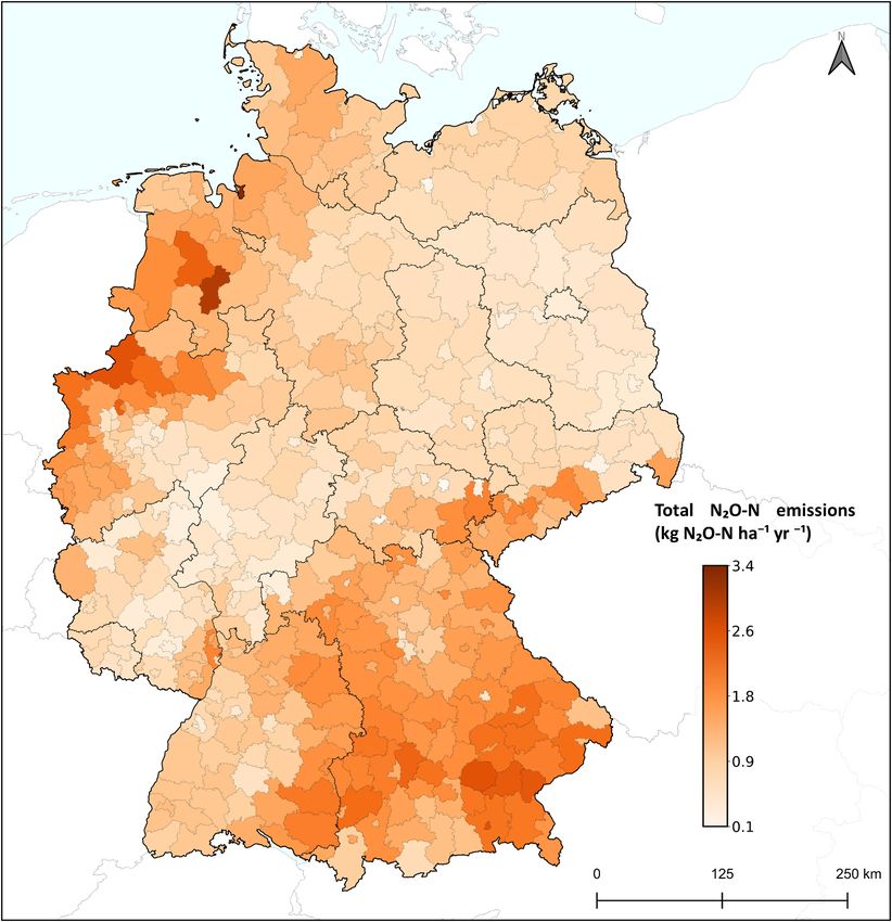
Fig. 4. District-wise N2O-N emissions related to agricultural area (kg N2O-N ha− 1). Borders of federal states and districts are indicated.
3.4. Unified emissions from mineral & organic soils generally higher than those of the two northern zones. Organic soils are
prevalent in the north as well as close to the Alps, i.e. Germany’s
The district-wise unified emission factor resulting from the weighted southern border, and can be clearly seen as increased emission factors
average of EFs associated with mineral (Model 4) and organic (Model 6) within the climatic zones. District-wise N inputs, i.e. the sum of synthetic
soils is shown in Fig. 3b. The EFs ranged from 0.38% to 0.92% across the fertiliser, animal manure, sewage sludge, biogas digestate and crop
country, with EFs for the south-west and south-east environmental zones residue inputs, in 2015 showed a pattern almost opposite to that of the
9G.P. Mathivanan et al. Agriculture, Ecosystems and Environment 322 (2021) 107640
Table 2 4. Discussion
Comparison of Tier 1 (IPCC, 2006, 2019, aggregated Tier 1 value) and Tier 2
(this study) implied emission factors and corresponding N2O emissions for 2015 The new N2O EFs for Germany confirmed the initial hypothesis of
(submission 2021). this study that N2O emissions are overestimated by the IPCC’s default
GHG sources Tier 1 Tier 2 1% EF. The lower magnitude of N2O emissions is in agreement with Tian
Implied N2O Implied N2O et al. (2020), where estimates from the bottom-up approach used for
emission emissions emission emissions national GHG inventories in Europe are higher overall than top-down
factors (kg (kt) factors (kg (kt) estimates. In comparison with Tier 2 EFs for other countries, Ger
N2O-N/kg N2O-N/kg many’s new direct N2O IEF for inorganic fertilisers is similar to that of
N) N)
Japan, New Zealand and the United Kingdom, while countries such as
Inorganic N 0.01 27.28 0.0061 16.69 Ireland, the Netherlands, the Russian Federation and the USA report
fertilisers (0.0042 –
IEFs above 1% (UNFCCC, 2021). The IEF for organic fertilisers was
0.0084)
Animal manure 0.01 15.38 0.0066 10.13 almost the same as that for inorganic fertilisers, and was comparable
applied to soils (0.0046 – with those of Japan and the United Kingdom.
0.0090) This variability of EFs with respect to geographical locations not only
Sewage sludge 0.01 0.29 0.0057 0.17 exists between countries but also within Germany, with measured N2O
applied to soils (0.0041 –
0.0077)
emissions generally being low in the north-east and substantially higher
Other organic 0.01 4.77 0.0065 3.08 in the south-east. The differing emission factors in different regions have
fertilisers (0.0045 – previously been explained by the effect of climatic conditions, soil
applied to soils 0.0087) properties such as soil aeration, pH, and agricultural land use (Dechow
(digestates)
and Freibauer, 2011; Jungkunst et al., 2006). Consequently, environ
Crop residues 0.01 9.57 0.0059 5.67
(0.0041 – mental stratification, which integrates climate and geomorphology, is a
0.0081) good predictor in the derived empirical models.
Overall 0.01 (0.003 – 57.29 0.0062 35.74 In contrast to what is reported by other countries in their inventories
(Uncertainty 0.03; 0.001 – (0.0043 – and what is suggested in the 2019 IPCC Refinement, the extensive data
ranges: IPCC, 0.018) 0.0085)
2006; IPCC,
from Germany do not support different EFs for synthetic and organic
2019) fertilisers. There are reasons for expecting lower EFs for organic N input.
Larger ammonia losses from organic fertilisers than from synthetic fer
tilisers result in less nitrogen available for N2O production. Furthermore,
EFs, with the districts to the north of Germany and a few districts in the extensive agriculture with low N surplus (such as organic farming sys
south having the highest N fertiliser application rates up to 59.2 Gg N tems) use organic fertilisation but not synthetic fertilisers. However,
yr− 1 (Fig. 3a). Unlike the EFs, where most of the high figures were there are also arguments against lower EFs for organic N inputs. Slower
concentrated in the south, the total N2O emissions from all N sources N uptake by crops after organic fertiliser application and the longer time
displayed a divergent pattern, with the district of “Emsland” in north- span over which organic nitrogen is mineralised in soils provide op
west Germany having the highest emission of 0.35 Gg N2O-N yr− 1 portunities for N2O production (Petersen, 1999; Velthof et al., 2003).
(Fig. 3c) due to high N inputs combined with a large proportion of Unfortunately, studies in the database that compared synthetic and
organic soils. Lower N2O emissions were predominantly estimated for organic fertilisers were usually not optimally set up for EFs to be
the west-central districts, which are mostly urban areas and have lower compared. Several treatments of varying N input would be needed for
N fertiliser application rates. Overall, the national total direct N2O both fertiliser types. It is therefore possible that the effect of fertiliser
emissions from the five N sources in 2015 were estimated to be 22.75 Gg type also exists in Germany and would become evident if more dedicated
N2O-N yr− 1, of which synthetic fertilisers contributed 10.62 Gg N2O-N experiments were conducted. However, the present study showed that
yr− 1 followed by animal manure at 6.45 Gg N2O-N yr− 1. Emissions from emissions from synthetic fertilisers are not as high as the levels sug
other N sources, i.e. sewage sludge, biogas digestates and crop residues gested by the 2019 IPCC refinement (IPCC, 2019).
were 0.11, 1.96 and 3.61 Gg N2O-N yr− 1 respectively. There has been considerable debate over whether the N2O response
Generally, crop production and thus N inputs are higher in the to N input is non-linear. Kim et al. (2013b) and Shcherbak et al. (2014)
northern zones than the south (Fig. 3a). However, the southern envi conducted meta-analyses and found a trend of N2O emissions increasing
ronmental zones had higher emission factors than the north (Fig. 3b). As exponentially if N input exceeds crop needs. Screening of the data
a result, relatively high district-wise total N2O emissions are estimated collected from Germany did not reveal this non-linearity, but most of the
for the north and the south-east regions (Fig. 3c). When relating N2O studies were focused on recommended fertilisation practices, thus
emissions to agricultural area, high values occur in the north-west, over-fertilisation is likely to be rare in the dataset. A linear relationship
which is a region of concentrated livestock farming (Statistisches Bun was therefore assumed for modelling purposes. There are substantial
desamt (Destatis), 2020), and in the south-east region (Fig. 4). advantages of a linear relationship for an inventory because the models
The national implied EFs were similar for all N sources, with 0.7% for can be upscaled simply by using aggregated values for N input. A
animal manure and biogas digestates and 0.6% for synthetic fertilisers, non-linear model that is calibrated on field-scale data cannot be
sewage sludge and crop residues (Table 2). The difference between EFs upscaled to district-scale as easily as a linear model.
for synthetic fertilisers and animal manure is a function of the spatial Jungkunst et al. (2006) highlight that the correlation between soil
distribution of the N sources between organic and mineral soils. For properties and N2O emissions, which commonly exists on a site-specific
instance, the north-west region with high concentration of livestock is scale, decreases at a national level. Although the inclusion of soil
also a region with higher concentration of organic soils (Fig. S1). The properties and crop types, the latter being a proxy for timing of fertil
overall implied emission factor was 0.62% (0.43–0.85%) which is isation and N uptake as well as the quality of crop residues, slightly
significantly lower and has a narrower uncertainty range than both the improved the model’s predictive performance, generally the effects
default Tier 1 EF of 1% (0.3− 3%) currently used and the IPCC (2019) were rather uncertain. The effect of soil properties on EF could not be
Tier 1 EF of 1% (0.1–1.8%). The implied emission factor for synthetic included in the empirical model because the model became
fertilisers (0.61%) was also considerably lower than the proposed IPCC over-parameterised and impossible to fit successfully. It would be pref
(2019) stratified EF for synthetic fertilisers 1.6% (1.3–1.9%). erable to use a process model to quantify these effects, but sufficient
fine-scaled data are not available for Germany’s emission inventory and
10G.P. Mathivanan et al. Agriculture, Ecosystems and Environment 322 (2021) 107640
thus fitting a process model was beyond the scope of this study. An emission sources in agriculture, including N2O emissions from soils, will
empirical model was not fitted on soil data at a district level because soil need to be mitigated if the ambitious goals of climate protection policy
properties are difficult to aggregate for districts and can vary consider (Deutscher Bundestag, 2019; European Commission, 2020) are to be
ably, e.g. pH within a district varies due to pH management. That kind of achieved.
a model can therefore be expected to have a worse predictive perfor
mance than the simpler model that only stratifies by environmental
Declaration of Competing Interest
zones. A model adding only crop type as predictor was not considered
for the inventory because the annual spatial distribution of crop types in
The authors declare that they have no known competing financial
Germany is not available for the whole time series from 1990.
interests or personal relationships that could have appeared to influence
Furthermore, winter crops are the main crops in Germany and therefore
the work reported in this paper.
also had the largest proportion of data points in the N2O database.
According to the model results, expected N2O emissions at zero fer
Acknowledgements
tilisation were between 1.4 kg N ha− 1 yr− 1 in the north and 2.0 kg N
ha− 1 yr− 1 in the south of Germany on mineral soils and about 4.6 kg N
We thank Heinz Flessa, for his valuable comments on the draft of the
ha− 1 yr− 1 on organic soils. In their global meta-analysis, Kim et al.
manuscript. Also, we appreciate the contribution of Claire Tarring in
(2013a) observed a mean background emission of 1.5 kg N ha− 1, but
editing the style and language of the manuscript. The remaining lan
reported a higher value of 2.4 kg N ha− 1 for Germany. Unfortunately, no
guage mistakes, if any, were made by the authors.
distinction was made between mineral and organic soils. However,
background emissions from agricultural land are more of an experi
Appendix A. Supporting information
mental artefact because unfertilised controls are not representative of
good agricultural practice. Kim et al. (2013a) list several drivers of
Supplementary data associated with this article can be found in the
background emissions: fertilisation and soil management in previous
online version at doi:10.1016/j.agee.2021.107640.
years, atmospheric N deposition and plant residues. Furthermore, N2O
emissions can result from mineralisation of soil organic matter, which
also interacts with fertilisation (Craine et al., 2007). A strong correlation References
was observed between the background emissions from the environ
Ackermann, A., Mahnkopf, J., Heidecke, C., Venohr, M., 2016. Reducing agricultural
mental zones and their emission factors (R2 = 0.96). This suggests that nitrogen inputs in the German Baltic Sea catchment - trends and policy options.
environmental controls of N2O production differ more between these Water Sci. Technol. J. Int. Assoc. Water Pollut. Res. 74, 1060–1068. https://doi.org/
regions than the availability of nitrogen in control treatments, particu 10.2166/wst.2016.267.
Bouwman, A.F., 1996. Direct emission of nitrous oxide from agricultural soils. Nutr. Cycl.
larly in newly established unfertilised plots. Agroecosyst. 46, 53–70. https://doi.org/10.1007/bf00210224.
Since N2O emissions were only modelled as a function of exogenous Brown, P., Cardenas, L., Choudrie, S., Del Vento, S., Karagianni, E., MacCarthy, J.,
nitrogen (excluding N deposition) and endogenous sources and legacy Mullen, P., Passant, N., Richmond, B., Smith, H., Thistlethwaite, G., Thomson, A.,
Turtle, L., Wakeling, D., 2021, UK Greenhouse Gas Inventory, 1990 to 2019. 〈http
effects cannot be disentangled, the new EF was only applied to inputs of s://uk-air.defra.gov.uk/assets/documents/reports/cat09/2105061125_ukghgi-9
synthetic fertilisers, organic fertilisers, biogas digestates, sewage sludge 0–19_Main_Issue_1.pdf〉.
and crop residues. Although crop residues were not included in the N Butterbach-Bahl, K., Baggs, E.M., Dannenmann, M., Kiese, R., Zechmeister-
Boltenstern, S., 2013. Nitrous oxide emissions from soils: how well do we understand
input of the calibration data, the example set by IPCC was followed and the processes and their controls? Philos. Trans. R. Soc. Lond. B Biol. Sci. 368,
it was assumed that the EF was also valid for this N input. This was 20130122 https://doi.org/10.1098/rstb.2013.0122.
supported by the correlation between background emissions and EFs, as COP, 2015, Adoption of the Paris Agreement, 21st Conference of the Parties. 〈https://un
fccc.int/sites/default/files/english_paris_agreement.pdf〉.
crop residues are likely to be a large part of N input not accounted for in
Craine, J.M., Morrow, C., Fierer, N., 2007. Microbial nitrogen limitation increases
the dataset. However, we are not confident that the new EFs are appli decomposition. Ecology 88, 2105–2113. https://doi.org/10.1890/06-1847.1.
cable to nitrogen from a very slow release process such as mineralisation Dechow, R., Freibauer, A., 2011. Assessment of German nitrous oxide emissions using
empirical modelling approaches. Nutr. Cycl. Agroecosyst. 91, 235–254. https://doi.
of soil organic matter or to non-agricultural areas. It is therefore rec
org/10.1007/s10705-011-9458-9.
ommended that, until further research findings are available, the IPCC Deutscher Bundestag, 2019, Gesetz zur Einführung eines Bundes-Klimaschutzgesetzes
default EF for direct N2O emissions from the mineralisation of soil und zur Änderung weiterer Vorschriften (German Climate Protection Law). 〈htt
organic matter should be continued to be used in Germany’s emission p://www.bgbl.de/xaver/bgbl/start.xav?startbk=Bundesanzeiger_BGBl&jumpTo=b
gbl119s2513.pdf〉.
inventory. Düngeverordnung, 2021, Düngeverordnung (German fertiliser ordinance) of May 26,
2017 (Bundesgesetzblatt I p.1305), last changed on August 10, 2021
5. Conclusions (Bundesgesetzblatt I p.3436). 〈https://www.gesetze-im-internet.de/d_v_2017/〉.
Environment and Climate Change Canada, 2021, National Inventory Report 1990–2019:
Greenhouse Gas Sources and Sinks in Canada. Canada. 〈https://publications.gc.ca/si
According to the new methodology in this study, the new best esti te/eng/9.506002/publication.html〉.
mate of GHG emissions from German agriculture in 2015 is 5.71 Tg CO2- European Commission, 2020, COMMUNICATION FROM THE COMMISSION TO THE
EUROPEAN PARLIAMENT, THE COUNCIL, THE EUROPEAN ECONOMIC AND
eq. (8.59%) lower than that reported in 2021 submission (66.51 Mt CO2- SOCIAL COMMITTEE AND THE COMMITTEE OF THE REGIONS Stepping up
eq, converted with GWPs according to (IPCC, 2014a)). Inventory com Europe’s 2030 climate ambition Investing in a climate-neutral future for the benefit
pilers can easily apply this new method to the whole time series from of our people (No. COM/2020/562 final). 〈https://eur-lex.europa.eu/legal-content
/EN/TXT/?uri=CELEX:52020DC0562〉.
1990 to the present day, which would change the estimate of mitigation European Community, 2003, Regulation (EC) No 1059/2003 of the European Parliament
achieved in that period. As reported mitigation of N2O emissions from and of the Council of 26 May 2003 on the establishment of a common classification
soils between 1990 and 2019 (15.27%) was lower than GHG mitigation of territorial units for statistics (NUTS), OJ L. 〈http://data.europa.eu/eli/reg
/2003/1059/oj/eng〉.
in the agricultural sector (19.63%, converted with GWPs according to European Environment Agency, 2021, Annual European Union greenhouse gas inventory
(IPCC, 2014a)), the smaller contribution of N2O emissions from soils to 1990–2019 and inventory report 2021 (No. EEA/PUBL/2021/066). 〈https://www.
total agricultural emissions results in a larger estimated sectoral miti eea.europa.eu/publications/annual-european-union-greenhouse-gas-inventor
y-2021〉.
gation. With the new EFs, the N2O mitigation from agricultural soils was
Federal Environment Agency, 2021, National Inventory Report for the German
marginally lower than the 2021 submission at 15.08%, while the sec Greenhouse Gas Inventory. 〈https://unfccc.int/documents/273433〉.
toral N2O mitigation increased to 19.94%. Furthermore, due to the Flessa, H., Wild, U., Klemisch, M., Pfadenhauer, J., 1998. Nitrous oxide and methane
smaller share of N2O emissions from soils, mitigation measures focusing fluxes from organic soils under agriculture. Eur. J. Soil Sci. 49, 327–335. https://doi.
org/10.1046/j.1365-2389.1998.00156.x.
on methane emissions from livestock farming will have a stronger Gocht, A., Röder, N., 2014. Using a Bayesian estimator to combine information from a
relative effect than measures for reducing N2O emissions. However, all cluster analysis and remote sensing data to estimate high-resolution data for
11You can also read


