Turbulent magnetic fields in the merging galaxy cluster MACS J0717.5+3745: polarization analysis
←
→
Page content transcription
If your browser does not render page correctly, please read the page content below
Astronomy & Astrophysics manuscript no. MACS_pol                                                                                    ©ESO 2021
                                               October 1, 2021

                                                             Turbulent magnetic fields in the merging galaxy cluster
                                                                   MACS J0717.5+3745: polarization analysis
                                                      K. Rajpurohit1, 2, 3 , M. Hoeft3 , D. Wittor4, 1 , R. J. van Weeren5 , F. Vazza1, 2, 4 , L. Rudnick6 , W. R. Forman7 ,
                                                  C. J. Riseley1, 2, 8 , M. Brienza1, 2 , A. Bonafede1, 2, 4 , A. S. Rajpurohit9 , P. Domínguez-Fernández10 , S. Rajpurohit11 ,
                                               J. Eilek13, 14 , E. Bonnassieux1, 2 , M. Brüggen4 , F. Loi12 , H. J. A. Röttgering5 , A. Drabent3 , N. Locatelli1, 2 , A. Botteon5 ,
                                                                                                   G. Brunetti2 , T. E. Clarke15

                                                      1
                                                          Dipartimento di Fisica e Astronomia, Universitá di Bologna, Via P. Gobetti 93/2, 40129, Bologna, Italy
                                                          e-mail: kamlesh.rajpurohit@unibo.it
arXiv:2109.15237v1 [astro-ph.CO] 30 Sep 2021

                                                      2
                                                          INAF-Istituto di Radio Astronomia, Via Gobetti 101, 40129, Bologna, Italy
                                                      3
                                                          Thüringer Landessternwarte (TLS), Sternwarte 5, 07778 Tautenburg, Germany
                                                      4
                                                          Hamburger Sternwarte, Universität Hamburg, Gojenbergsweg 112, 21029, Hamburg, Germany
                                                      5
                                                          Leiden Observatory, Leiden University, P.O. Box 9513, 2300 RA Leiden, The Netherlands
                                                      6
                                                          Minnesota Institute for Astrophysics, University of Minnesota, 116 Church St. S.E., Minneapolis, MN 55455, USA
                                                      7
                                                          Harvard-Smithsonian Center for Astrophysics, 60 Garden Street, Cambridge, MA 02138, USA
                                                      8
                                                          CSIRO Astronomy and Space Science, PO Box 1130, Bentley, WA 6102, Australia
                                                      9
                                                          Astronomy & Astrophysics Division, Physical Research Laboratory, Ahmedabad 380009, India
                                                     10
                                                          Department of Physics, School of Natural Sciences UNIST, Ulsan 44919, Korea
                                                     11
                                                          Molecular Foundry, Lawrence Berkeley National Laboratory, CA 94720, USA
                                                     12
                                                          INAF-Osservatorio Astronomico di Cagliari, Via della Scienza 5, 09047 Selargius, CA, Italy
                                                     13
                                                          Department of Physics, New Mexico Tech, Socorro, NM 87801, USA
                                                     14
                                                          National Radio Astronomy Observatory, Socorro, NM 87801, USA
                                                     15
                                                          U.S. Naval Research Laboratory, 4555 Overlook Avenue SW, Washington, D.C. 20375, USA

                                                    October 1, 2021

                                                                                                                 ABSTRACT

                                                    We present wideband (1−6.5 GHz) polarimetric observations, obtained with the Karl G. Jansky Very Large Array (VLA), of the
                                                    merging galaxy cluster MACS J0717.5+3745, which hosts one of the most complex known radio relic and halo systems. We use both
                                                    Rotation Measure Synthesis and QU-fitting, and find a reasonable agreement of the results obtained with these methods, in particular,
                                                    when the Faraday distribution is simple and the depolarization is mild. The relic is highly polarized over its entire length (850 kpc),
                                                    reaching a fractional polarization >30% in some regions. We also observe a strong wavelength-dependent depolarization for some
                                                    regions of the relic. The northern part of the relic shows a complex Faraday distribution suggesting that this region is located in or
                                                    behind the intracluster medium (ICM). Conversely, the southern part of the relic shows a Rotation Measure very close to the Galactic
                                                    foreground, with a rather low Faraday dispersion, indicating very little magnetoionic material intervening the line-of-sight. From
                                                    spatially resolved polarization analysis, we find that the scatter of Faraday depths correlates with the depolarization, indicating that
                                                    the tangled magnetic field in the ICM causes the depolarization. We conclude that the ICM magnetic field could be highly turbulent.
                                                    At the position of a well known narrow-angle-tailed galaxy (NAT), we find evidence of two components clearly separated in Faraday
                                                    space. The high Faraday dispersion component seems to be associated with the NAT, suggesting the NAT is embedded in the ICM
                                                    while the southern part of the relic lies in front of it. If true, this implies that the relic and this radio galaxy are not necessarily
                                                    physically connected and thus, the relic may be not powered by the shock re-acceleration of fossil electrons from the NAT. The
                                                    magnetic field orientation follows the relic structure indicating a well-ordered magnetic field. We also detect polarized emission in
                                                    the halo region; however the absence of significant Faraday rotation and a low value of Faraday dispersion suggests the polarized
                                                    emission, previously considered as the part of the halo, has a shock(s) origin.
                                                    Key words. Galaxies: clusters: individual (MACS J0717.5+3745) − Galaxies: clusters: intracluster medium − large-scale structures
                                                    of universe − Acceleration of particles − Radiation mechanism: non-thermal: magnetic fields

                                               1. Introduction                                                           strength, topology, and evolution of these fields is poorly con-
                                                                                                                         strained.
                                               Magnetic fields are pervasive throughout the Universe and play                The strongest evidence of cluster-wide magnetic fields
                                               a vital role in numerous astrophysical processes: from our so-            comes from radio observations that have revealed large
                                               lar system up to filaments and voids in the large-scale structure         megaparsec-size, diffuse synchrotron emitting sources known as
                                               (e.g., Klein & Fletcher 2015; Beck 2015). Even the largest viri-          radio relics and halos (see van Weeren et al. 2019, for a recent
                                               alized structures in the Universe, galaxy clusters, are permeated         review). The presence of large-scale magnetic fields may have
                                               by magnetic fields (see Carilli & Taylor 2002; Govoni & Fer-              important implications for the different processes observed in
                                               etti 2004; Donnert et al. 2018, for reviews). However, the actual         galaxy clusters. A detailed analysis of the diffuse radio sources
                                                                                                                                                                    Article number, page 1 of 22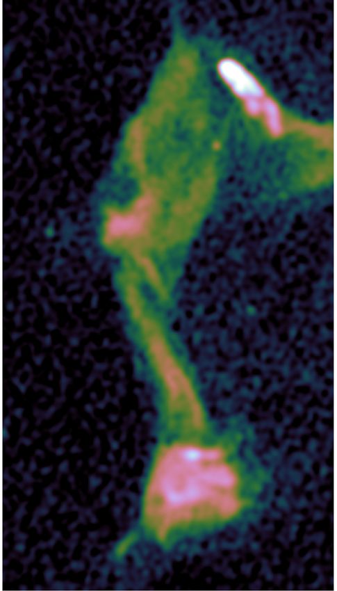
A&A proofs: manuscript no. MACS_pol

in clusters may help to shed light on the origin of the magnetic        presented in Sect. 4. This is followed by a detailed analysis and
fields, for example to determine if -as widely believed- very           discussion from Sects. 5 to 12. We summarize our main findings
weak seed fields are amplified by a dynamo process in the intra-        in Sect. 13.
cluster medium (ICM) and to determine how the magnetic fields               Throughout this paper, we assume a ΛCDM cosmology with
impact the physics of the ICM.                                          H0 = 70 km s−1 Mpc−1 , Ωm = 0.3, and ΩΛ = 0.7. At the cluster’s
     Radio relics are found in the periphery of merging galaxy          redshift, 100 corresponds to a physical scale of 6.4 kpc. All output
clusters and they often show irregular and filamentary morpholo-        images are in the J2000 coordinate system and are corrected for
gies (e.g., Owen et al. 2014; van Weeren et al. 2017b; Rajpuro-         primary beam attenuation.
hit et al. 2018; Di Gennaro et al. 2018; Rajpurohit et al. 2020a).
Relics trace shock waves occurring in the ICM during cluster
merger events (e.g., Sarazin et al. 2013; Ogrean et al. 2013; van       2. MACS J0717.5+3745
Weeren et al. 2016a; Botteon et al. 2016; Botteon et al. 2018).
                                                                        The galaxy cluster MACS J0717.5+3745 (l = 180.25° and b =
     It is believed that the cosmic ray electrons (CRe), which
                                                                        +21.05° ) located at z = 0.5458, hosts one of the most complex
form the radio relics via synchrotron emission, originate from a
                                                                        and powerful known relic-halo systems. (e.g., Bonafede et al.
first-order Fermi process, namely, Diffusive Shock Acceleration
                                                                        2009; van Weeren et al. 2009; Pandey-Pommier et al. 2013; van
(DSA, e.g., Blandford & Eichler 1987; Drury 1983; Ensslin et al.
                                                                        Weeren et al. 2017b; Rajpurohit et al. 2021c,a). The relic consists
1998; Hoeft & Brüggen 2007). The DSA at the shocks causing
                                                                        of four subregions, which have historically been referred to as
relics may also re-accelerate a pool of mildly relativistic fossil
                                                                        R1, R2, R3, and R4; see Fig 1. The relic is known to be polarized
electrons, previously injected by active galactic nuclei (AGN:
                                                                        above 1.4 GHz and the polarization fraction varies along the relic
e.g., Bonafede et al. 2014; van Weeren et al. 2017a). The exis-
                                                                        (Bonafede et al. 2009).
tence of mildly relativistic electrons in front of the shock may
                                                                            High-resolution images from the VLA reveal that the relic
help to reconcile the low acceleration efficiency with the high
                                                                        has several filaments on scales down to 30 kpc. Some of these
radio luminosity for relics with weak shocks (Mach number ≤ 2,
                                                                        filaments originate from the relic itself, while a few of them, F1
e.g., Kang & Ryu 2011; Botteon et al. 2020). However, the exact
                                                                        and F2 (see Fig. 1) appear more isolated. Recently, it has been
spectral energy distribution and spatial distribution of such fossil
                                                                        reported that the relic consists of several fine overlapping struc-
electrons in the ICM are mostly unconstrained.
                                                                        tures with different spectral indices (Rajpurohit et al. 2021c).
     Radio relics are strongly polarized at frequencies above
                                                                        The curvature distribution suggests that the relic is very likely
1 GHz, some with a polarization fraction as high as 65% (e.g.,
                                                                        seen less edge-on with a viewing angle close to about 45°.
van Weeren et al. 2010, 2012; Owen et al. 2014; Kierdorf et al.
2017; Loi et al. 2020; Rajpurohit et al. 2020b; Di Gennaro et al.           At the center of the relic, there is an embedded Narrow An-
2021). The inferred magnetic field directions are often found to        gle Tail (NAT) galaxy (see Fig. 1). At high frequencies (above
be well aligned with the shock surface. However, the exact mech-        1 GHz), the tails of the NAT seem to fade into the R3 region of
anism causing the high degree of polarization and the aligned po-       the relic (van Weeren et al. 2017b). However, at low frequencies
larization angle is still unclear. The alignment could be caused        (below 750 MHz), the tails are apparently bent to the south of the
by a preferentially tangential magnetic field orientation or by         R3 region (Rajpurohit et al. 2021c). It is not clear if this morpho-
the compression of a small-scale tangled magnetic field at shock        logical connection between the NAT and the relic is physical or
(Laing 1980; Ensslin et al. 1998).                                      they are simply two different structures projected along the same
                                                                        line-of-sight (van Weeren et al. 2017b; Rajpurohit et al. 2021c).
     Unlike relics, radio halos are typically unpolarized sources
                                                                        If this connection is physical this may suggest that the relic is
located at the center of a cluster. The radio emission from halos
                                                                        powered by the shock re-acceleration of mildly relativistic fos-
roughly follows the X-ray emission (e.g., Pearce et al. 2017; Ra-
                                                                        sil electrons from the NAT. The Fanaroff-Riley type I galaxy
jpurohit et al. 2018; van Weeren et al. 2017a). The currently fa-
                                                                        to the south of the MACS J0717.5+3745 shows a redshift of
vored scenario for the formation of radio halos involves the reac-
                                                                        zFRI = 0.1546, hence, not related to the cluster.
celeration of CRe to higher energies by turbulence induced dur-
ing mergers (e.g., Brunetti et al. 2001; Petrosian 2001; Brunetti           The cluster also hosts a powerful steep spectrum radio
& Jones 2014).                                                          halo with a largest linear size of about 2.6 Mpc (Bonafede
                                                                        et al. 2009; van Weeren et al. 2009; Pandey-Pommier et al.
     Polarized emission at the cluster outskirts is crucial to un-
                                                                        2013; van Weeren et al. 2017b; Bonafede et al. 2018; Rajpuro-
derstand the magnetic field properties of the ICM (see, Carilli &
                                                                        hit et al. 2021a). High resolution total power images taken
Taylor 2002; Govoni & Feretti 2004, for a review). The orien-
                                                                        with the VLA have shown the presence of several radio fil-
tation and topology of magnetic fields at merger shocks is im-
                                                                        aments of 100-300 kpc in extent within the halo region (van
portant to better understand the physics of shock acceleration,
                                                                        Weeren et al. 2017b). Uncommonly, for radio halos, the halo
because the efficiency of particle acceleration might be a strong
                                                                        in MACS J0717.5+3745 has previously been reported to be po-
function of the magnetic field topology upstream of the shock
                                                                        larized at the level of 2-7% at 1.4 GHz (Bonafede et al. 2009).
(e.g., Wittor et al. 2020). However, magnetic fields in the ICM
                                                                        However, it is unclear if the polarized emission reported in the
are notoriously difficult to measure, and the low-density regions
                                                                        central part of the halo is associated with the halo or not.
in the cluster outskirts are even more challenging to probe (John-
son et al. 2020).
     In this work, we describe the results obtained from polari-        3. Observations and Data Reduction
metric analysis of Karl G. Jansky Very Large Array (VLA) L-,
S-, and C-band observations covering the 1-6.5 GHz frequency            VLA wideband observations of MACS J0717.5+3745 were ob-
range. The enormous wideband information and remarkable res-            tained in L-band (ABCD-array configuration), S-band (ABCD-
olution allow us to carry out spatially resolved polarimetric stud-     array configuration), and C-band (BCD-array configuration),
ies, providing crucial insights into the ICM magnetic fields.           covering the frequency range from 1 to 6.5 GHz. For observation
     The outline of this paper is as follows: in Sect. 3, we describe   details and description of the data reduction procedure, we refer
the observations and data reduction. The polarization images are        the reader to van Weeren et al. (2016b, 2017b). While previous
Article number, page 2 of 22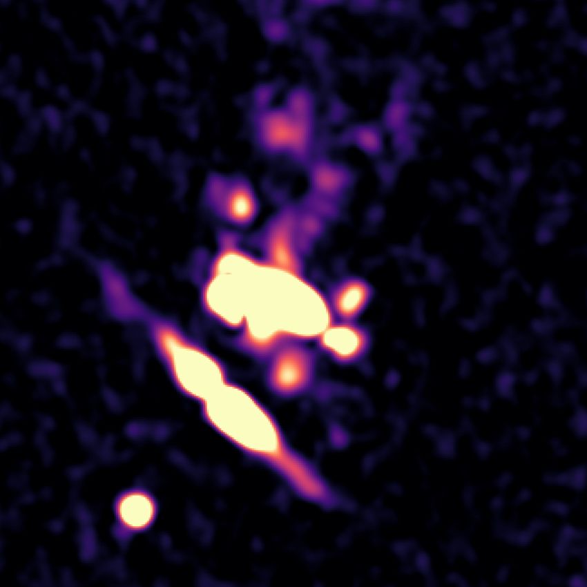
Rajpurohit et al.: MACS J0717.5+3745: polarization analysis

Table 1. Image properties

         Band               Configuration           Name           Restoring Beam                            RMS noise
                                                                                             Stokes I (σrms )      Stokes QU (σQU )
                                                                                              µ Jy beam−1             µ Jy beam−1
                                 BCD                 IM1             2.000 × 2.000                 1.4                     1.2
    VLA C-band †                 BCD                 IM2             4.000 × 4.000                 1.8                     1.4
    (4.5-6.5 GHz)               BCD                  IM3             5.000 × 5.000                 1.9                     1.5
                                 BCD                 IM4            12.500 × 12.500                7.2                     5.9
                                ABCD                 IM5             2.000 × 2.000                 1.1                     0.9
     VLA S-band†                ABCD                 IM6             4.000 × 4.000                 1.7                     1.0
      (2-4 GHz)                 ABCD                 IM7             5.000 × 5.000                 1.8                     1.1
                                ABCD                 IM8             1200. 5 × 1200. 5             8.2                     6.1
                                ABCD                 IM9             2.000 × 2.000                 3.2                     2.7
     VLA L-band†                ABCD                IM10             4.000 × 4.000                 6.0                     3.2
      (1-2 GHz)                 ABCD                IM11             5.000 × 5.000                 6.8                     3.4
                                ABCD                IM12            12.500 × 12.500               12.4                    10.1
 Notes. For full wideband Stokes IQU maps, imaging was performed using multi-scale clean, nterms=2 and wprojplanes=500. All Stokes
IQU images are made with Briggs weighting with robust = 0. For making all channelized Stokes IQU images at 400 , 500 , and 12.500 resolutions,
we used nterms=1 and robust = 0.0; † For data reduction steps, we refer to van Weeren et al. (2016b, 2017b).

analysis of the data only considered the total power, the VLA            where σQU is the average noise of Stokes Q and U images and
observations were taken in full-polarization mode, allowing us           the index ‘meas’ indicates the measured property, unavoidably
to investigate the polarization properties of the cluster.               including a noise, for clarity. The uncertainties in the flux density
    The data reduction and imaging were performed with CASA.             measurements were estimated as:
The data were calibrated for antenna position offsets, elevation-               q
dependent gains, parallel-hand delay, bandpass, and gain varia-          ∆S ν = ( f · S ν )2 + Nbeams · σ2rms ,                            (3)
tions using 3C147. For polarization calibration, the leakage re-
sponse was determined using the unpolarized calibrator 3C147.            where f is an absolute flux density calibration uncertainty, S ν is
The cross-hand delays and the absolute polarization position an-         the flux density, σrms is the RMS noise, and Nbeams is the number
gle were corrected using 3C138. Finally, the calibration solu-           of beams covered by the source. We assume absolute flux density
tions were applied to the target field and the resulting calibrated      uncertainties of 4% for the VLA L-band and 2.5% for the VLA
data were averaged by a factor of 4 in frequency per spectral win-       S- and C-bands (Perley & Butler 2013).
dow. Several rounds of self-calibration were performed to refine
the gain solutions. After the individual data sets were calibrated,      4. Polarized emission
the observations from the different configurations (for the same
frequency band) were combined and imaged together.                       In Fig. 2, we show the high-resolution, that is 200 , polarized in-
    We produced Stokes I, Q, and U images of the target field            tensity maps of the relic for the VLA L-, S-, and C-band. Polar-
from the data at L-band, S-band, and C-band, including data              ized emission from the relic subregions (R1, R2, R3, and R4) is
from all array configurations. Deconvolution was done with               detected in all three frequency bands.
CLEAN masks generated in the PyBDSM (Mohan & Rafferty                        The polarized emission more or less follows the structure
2015). Imaging was always performed with Briggs weighting                seen in the total intensity images; however, the polarized emis-
(Briggs 1995) using robust = 0.0 and all images were corrected           sion seems to be more ‘clumpy’ compared to the total power
for primary beam attenuation, see Table 1 for the properties of          emission. Moreover, we find that there are fluctuations in the po-
the images obtained. For Faraday analysis, the full 1-6.5 GHz            larization intensity, in particular for the northern part of the relic
channel with Stokes IQU cubes were imaged to a common res-               (R1 and R2), on scale as small as 10 kpc. The polarized inten-
olution of 400 , 500 and 12.500 resolutions. These IQU cubes were        sity map in Fig. 2 also indicates that in L-band the polarized flux
inspected and any spectral channels which showed large arti-             density in the northern part of the relic is low compared to the
facts or a large increase in noise compared to the average were          southern part (R3 and R4). To investigate this further, we create
excluded. We note that the highest common resolution possible            maps for the fractional polarization p = |P|/I.
with our L-, S- and C-bands VLA data was 400 , therefore 200 res-            The L-, S-, and C-band high resolution (200 ) fractional po-
olution Stokes IQU cubes were not used for Faraday analysis.             larization maps of the relic are shown in Fig. 3. At such a high
    The polarized flux density was computed from the Stokes Q            resolution, the relic is polarized over its entire length in C-band.
and U flux densities according to the definition of polarization         We find that in all three bands the polarization fraction across the
as a complex property                                                    relic varies significantly, from unpolarized to a maximum frac-
                                                                         tional polarization of about 50 % in C-band.
P = Q + iU,                                                       (1)        An overview of the polarization properties of the diffuse ra-
where the absolute of P results in the polarized flux density.           dio sources in the cluster is given in Table 2. We measure the av-
Since both, Q and U, are affected by noise in the measurement,           erage fractional polarization in the four subregions of the relic.
we correct the polarized flux density, |P|, for the Rician bias          These regions are shown in the left panel of Fig. 4. The spatially
(Wardle & Kronberg 1974) as:                                             averaged polarization fraction over R1 is (21 ± 2) % in C-band.
      q                                                                  The fractional polarization drops quickly towards lower frequen-
|P| = Q2meas + Umeas
                 2
                      − 2.3 σ2QU ,                          (2)          cies, reaching as low as (3 ± 1) % in L-band. Similar trends are
                                                                                                                  Article number, page 3 of 22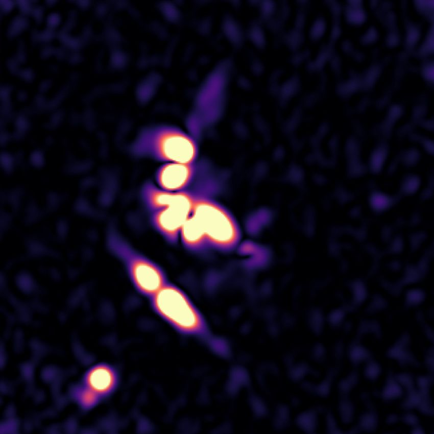
A&A proofs: manuscript no. MACS_pol
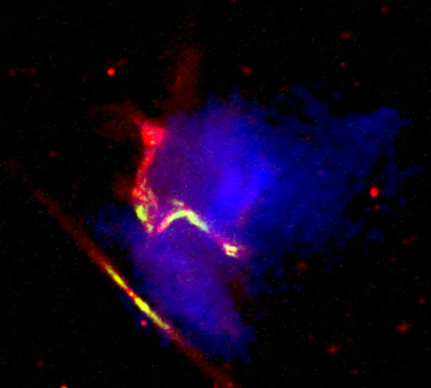
F1
R1
R2
F2
R3
NAT core
R4
FRI
Fig. 1. Composite total power, polarization intensity, and X-ray image of the relic in MACS J0717+3745 at 200 resolution. The total power and L-
band polarization emission are shown in red and green-yellow, respectively. The intensity in blue shows the X-ray emission. The lack of polarized
emission in the north region (R1) indicates depolarization. The image properties are given in Table 1, IM5 and IM9.
noticed for the R2 region of the relic. We observe large local opposite trends (i.e., polarization fraction increasing toward the
fluctuations in the polarization fraction in particular for R1 and downstream region of a shock front) is expected if the medium
R2. is uniform (Domínguez-Fernández et al. 2021).
From Table 2, the average fractional polarization of the R3
Looking at the high-resolution fractional polarization images
region ((28 ± 3) % at C-band) is highest compared to the rest
from C-band to L-band (Fig. 3), the average fractional polariza-
of the relic. In the region where the NAT is located we find a
tion of the relic in MACS J0717.5+3745 also increases in L-band
very low fractional polarization in all three bands. For the relic,
and S-band from R1 to R3. We find that the degree of polariza-
the average polarization fraction at R4 is the lowest (15 ± 1 % at
tion decreases generally with increasing wavelength.
C-band).
In the right panel of Fig. 4, we show the polarization frac- We also create polarization maps at 500 resolution. The result-
tion profile extracted from 200 maps at 1.5 GHz and 3 GHz. The ing maps at 1.5 GHz, 3 GHz, and 5.5 GHz are shown in Fig. 5.
corresponding regions are shown with green in the left panel of We note that that these polarization intensity maps are obtained
Fig. 4. In the R3 region there is a hint that the fractional po- by applying the Rotation Measure Synthesis (RM-synthesis:
larization decreases from south to north. Recently, Di Gennaro Brentjens & de Bruyn 2005, discussed in Sect. 5.1). In these
et al. (2021) found that the polarization fraction decreases toward maps, we find additional low surface brightness polarized emis-
the downstream of the entire Sausage relic. Simulations show sion, in particular in filamentary features F1 and F2 (see Fig. 1
that such trends are expected in a turbulent medium while the for labeling). The two filaments are highly polarized at all the
Article number, page 4 of 22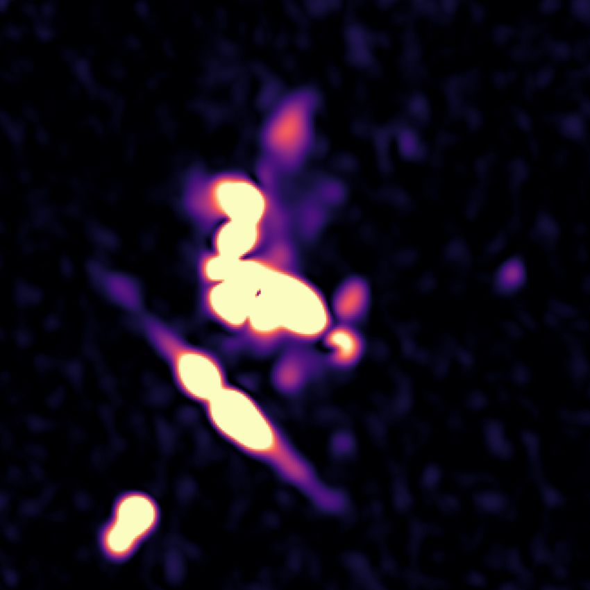
Rajpurohit et al.: MACS J0717.5+3745: polarization analysis

                                       Polarized Intensity [mJy beam 1]                               Polarized Intensity [mJy beam 1]                          Polarized Intensity [mJy beam 1]
                          0.01   0.02     0.03     0.04   0.05   0.06         0.07   0.08   0.01      0.02   0.03     0.04    0.05     0.06    0.07       0.01              0.02         0.03            0.04
              37°46'30"      150 kpc                                                        150 kpc                                                   150 kpc
                                                                               1-2 GHz                                                     2-4 GHz                                              4.5-6.5 GHz

                   00"
Declination

                 45'30"

                   00"

                             7h17m38s        36s          34s           32s          30s    7h17m38s         36s        34s          32s        30s   7h17m38s        36s          34s      32s          30s
                             Right Ascension                             Right Ascension                                Right Ascension
 Fig. 2. Polarization intensity images of the relic in MACS J0717.5+3745 at 200 resolution, showing that the polarization emission√is distributed in a
 clumpy manner. The image also revels fine, small-scale filaments visible in the total power emission. Contour levels are drawn at [1, 2, 4, 8, . . . ] ×
 5σ rms and are from the VLA L-, S-, and C-band Stokes I images. The beam sizes are indicated in the bottom left corner of the each image. The
 image properties are given in Table 1, IM1, IM5, and IM9.

 observed frequencies, reaching values as high as (30 ± 2) % in                                                     they may serve as a powerful tool to disentangle the contribu-
 L-band, see Table 2.                                                                                               tion from different emission regions which are otherwise blended
     At 500 , the polarization fraction across the relic varies from                                                along the line-of-sight in continuum emission.
 about 2 %, that is the lowest value for a detection of polarized                                                       One of the most important physical effects to consider when
 emission in our maps, up to about 40 % between 1 and 5.5 GHz.                                                      discussing radio polarimetric observations is Faraday rotation.
 In Table 2, we also report the average fractional polarization                                                     It occurs when a radio wave on its way to the observer passes
 measured from 500 maps in the relic subregions. These values are                                                   through a magnetoionic medium which causes the polarization
 consistent with those reported by Bonafede et al. (2009) but are                                                   angle, ψobs , to vary as a function the wavelength (λ). The strength
 lower than measured from our 200 resolution maps. This implies                                                     of the Faraday effect is measured by the Rotation Measure (RM):
 that the degree of polarization increases with increasing resolu-
 tion, mainly by a factor of about 1.4 (for a resolution improving
                                                                                                                              dψobs
 by a factor of 2.5). At low resolution, regions with different po-                                                 RM =            .                                                                     (4)
 larization characteristics become blurred within a single resolu-                                                             dλ2
 tion element, leading to a loss of the observed polarized signal.                                                  We note that we use RM to exclusively indicate how rapidly the
 This effect is known as beam depolarization, and will be less if                                                   polarization angle changes with λ2 . In observations, the polar-
 the source is imaged at a higher resolution. Fig. 5 also shows a                                                   ization angle is obtained from the Stokes parameters Q and U of
 clear and sharp distinction between the main relic and the fila-                                                   linearly polarized emission via
 ments (F1 and F2), apparently protruding from the relic.                                                                               !
     As shown in Figs. 3 and 5, the average fractional polarization                                                         1         U
 across the relic increases from R1 to R3 also in L-band and S-                                                     ψobs = arctan          .                                     (5)
                                                                                                                            2         Q
 band. Moreover, the southern part of the relic is still significantly
 polarized in L-band. In contrast, the northern part of the relic
                                                                                                                       A magnetoionic medium causes a rotation of the polarization
 seems to be depolarized from C-band to L-band.
                                                                                                                    angle according to
     In Fig. 6, we show depolarization maps of the relic at 200
 and 500 resolutions. The depolarization is defined as DP = 1 −                                                     ∆ψ = ∆φ λ2 .                                                                          (6)
 p1.5 GHz /p5.5 GHz , where p1.5 GHz and p5.5 GHz are the fractional po-
 larization values at 1.5 GHz and 5.5 GHz, respectively. As evi-                                                    The difference in Faraday depth (∆φ) is given by integrating a
 dent, for the northern part of the relic, we find strong depolar-                                                  section of the light traveling path (∆l)
 ization (DP>0.6) between 1.5 GHz and 5.5 GHz. In particular,                                                                            Z
 the R1 region of the relic is almost fully depolarized at 1.5 GHz.                                                 ∆φ = 0.81 rad m   −2
                                                                                                                                             ne Bk dl ,                        (7)
 For the southern part, the depolarization (DP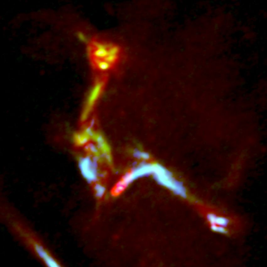
A&A proofs: manuscript no. MACS_pol

                                        Polarization fraction                                        Polarization fraction                                         Polarization fraction
                        0.1       0.2      0.3       0.4         0.5      0.6        0.1       0.2         0.3       0.4         0.5      0.6      0.1       0.2      0.3        0.4          0.5     0.6

                        150 kpc                                        1-2 GHz      150 kpc                                            2-4 GHz    150 kpc                                      4.5-6.5 GHz

              37°46'
Declination

                 45'

                       7h17m39s           36s              33s             30s      7h17m39s           36s                 33s             30s    7h17m39s           36s               33s             30s
                              Right Ascension                             Right Ascension                                Right Ascension
 Fig. 3. High resolution (200 ) fractional polarization maps at VLA L-, S-, and C-band. The relic is polarized at all of the observed frequen-
 cies,
 √ reaching values up to 50 % in some regions. The northern part of the relic strongly depolarizes at 1.5 GHz. Contour levels are drawn at
   [1, 2, 4, 8, . . . ] × 5σrms and are from the S-band Stokes I image. The beam sizes are indicated in the bottom left corner of the each image. The
 image properties are given in Table 1, IM1, IM5, and IM9.

 Table 2. Polarization properties of the diffuse radio emission in the cluster MACS J0717.5+3745.

                       Source                                                                VLA                                                                           Depolarization
                                                    C-band                                  S-band                                        L-band                               (DP)
                                                   hp5.5 GHz i                             hp3.0 GHz i                                   hp1.5 GHz i
                                            200                    500                200                    500                   200               500                   200               500
                                            %                      %                  %                      %                     %                 %
                        R1                21 ± 2                 15 ± 2             12 ± 2                  9±1                  3±1               2±1                 0.77                  0.90
                        R2                21 ± 2                 17 ± 2             20 ± 2                 16 ± 2                9±1               7±2                 0.46                  0.55
                        R3                28 ± 3                 20 ± 2             28 ± 2                 20 ± 2                16 ± 2            11 ± 1              0.30                  0.40
                        R4                15 ± 1                 10 ± 1             14 ± 1                  9±1                  9±1               6±1                 0.22                  0.24
                        F1                  −                    30 ± 2               −                    26 ± 2                  −               13 ± 1                -                     -
                        F2                  −                    24 ± 2               −                    22 ± 2                  −               14 ± 1                -                     -
                Notes. The fractional polarizations and DP are average values measured from 200 resolution L-, S-, and C-band fractional polarization
               and depolarization maps. The regions where the fractional polarization were extracted are indicated in the left panel of Fig. 4.

 allow to conclude on the Faraday depth distribution in a simple,                                                    Analyzing the Faraday rotation is a powerful method by
 straight forward way.                                                                                           which to investigate extragalactic magnetic fields. Observations
     Polarization studies of extragalactic sources have shown that                                               of the polarization angle as a function of frequency may provide
 a significant number of extended radio sources cannot be de-                                                    crucial information about the magnetization of the source and of
 scribed by a single component in Faraday depth (e.g., O’Sullivan                                                the medium intervening along the line-of-sight.
 et al. 2012; Anderson et al. 2015). Hence, the angle of Faraday
 rotation for multiple rotating or emitting screens along the line-
 of-sight is characterized by a distribution of Faraday depths (φ)                                                   Fundamental for this analysis is measuring the polarization
 instead of a single component. For a mixed Faraday rotating and                                                 angle over a wide range of wavelength. As discussed above,
 synchrotron emitting medium, the observed polarized intensity                                                   the polarization angle may depend in a complex way on wave-
 may originate from a large range of Faraday depths.                                                             length if there is polarized emission with a wide spread of Fara-
     The RM, as given in Eq. 4, determined in the observers                                                      day depths along the line-of-sight (Burn 1966; Tribble 1991;
 frame, would differ from similar measurements carried out                                                       Sokoloff et al. 1998). Faraday rotation may originate inside the
 closer to the source, for example in the rest-frame of the source,                                              radio emitting region, if enough thermal gas is mixed with the
 since the photons get redshifted from the source to the observer                                                synchrotron radiating plasma (internal Faraday dispersion). Al-
 due to the cosmological expansion (Kim et al. 2016; Basu et al.                                                 ternatively, it could be of external origin if magnetized thermal
 2018). Specifically, if in the rest-frame of the source, located at                                             gas is present along the line-of-sight (external Faraday disper-
 redshift zRM , a RM of RMint is determined, the cosmological ex-                                                sion).
 pansion would cause that in the observers frame an RM of
                          RMint                                                                                      The VLA L-, S-, and C-band data allow us to carry out a
 RMobs =                            ,                                                                (8)         detailed wideband polarization study of the compact and diffuse
                        (1 + zRM )2
                                                                                                                 radio sources in MACS J0717.5+3745. We used two methods to
 is found, if no magnetoionic medium is present along the line of                                                infer the Faraday distribution: Rotation Measure synthesis (RM-
 sight.                                                                                                          synthesis) and QU-fitting.
 Article number, page 6 of 22
Rajpurohit et al.: MACS J0717.5+3745: polarization analysis
50
1.5 GHz
1
45 3.0 GHz
2 3
6
4 5
7
40
Fractional polarization (%)
R1 8
10 9
11
12 35
13
14
16 17 18 38
15
19 20
40
39 30
21 22 23 24 R3
37 45
25 26 27 28 49
36 44 53
R2
29 30 31 35 43
47
48
52 56 25
32 34 42 46 51 55 58
33 41 50 54 57 59
R4
60
61
20
62
63
64
15
100 10 20 30 40 50 60
Distance from the shock (kpc)
Fig. 4. Left: VLA L-band image, blue regions show the relic subregions where the average fractional polarization was extracted. The fractional
polarization at R3 in Table 2 is obtained by excluding the contribution from the NAT. Red boxes where flux densities and Faraday dispersion
functions were extracted for QU-fitting and RM-synthesis, respectively. Each red box has a width of 500 , corresponding to a physical size of 32 kpc.
Right: The fractional polarization profile for the R3 region of the relic extracted from the green rectangular regions, shown in the left panel, of
width 200 . The total length of the each green region is about 50 kpc. At R3, there is a hint that the fractional polarization decreases in the downstream
region (i.e., from south to north as the shock front is expected at the leading southern edge for this part of the relic).
5.1. RM-synthesis two different resolutions, namely, 400 and 12.500 . The 400 reso-
lution cube was used to study the relic region while the low
The RM-synthesis technique, developed by Brentjens & de resolution 12.500 to study the low surface brightness polarized
Bruyn (2005), is based on the theoretical description of Burn emission features that are not detected at high resolution. The
(1966). RM-synthesis cube synthesized a range of Faraday depths from
The intensity of linearly polarized emission and its polariza- −800 rad m−2 to +800 rad m−2 , with a bin size of 2 rad m−2 . We
tion angle ψ can be expressed as a complex number used the entire L-, S-, and C-band data. These data give a sen-
P = I p0 e2iψ , (9) sitivity to the polarized emission up to a resolution in Faraday
depth (δφ) equal to
where I is the total intensity of the source and p0 is the fraction
of polarized emission. Following Burn (1966), the wavelength √
2 3
dependent polarization, P(λ2 ), can be written as a Fourier trans- δφ ≈ = 39 rad m−2 , (12)
form ∆λ2
Z ∞
P(λ2 ) = F(φ) e2iφ λ dφ,
2
(10) where, ∆λ2 = λ2max − λ2min . The high Faraday-space resolution
−∞ may allow us to separate multiple, narrowly-spaced, Faraday-
space components. We also run pyrmsynth individually only on
where φ is the Faraday depth which here became an independent
the L-, S-, and C-band data. The resulting polarization intensity
variable, forming the Faraday space. F(φ) is known as the Fara-
images for L-, S-, and C-band, overlaid with the total intensity
day dispersion function (FDF) and describes the amount of po-
contours are shown in Fig. 5.
larized emission originating from a certain Faraday depth. F(φ)
can be measured as The Faraday distribution of the relic in MACS J0717.5+3745
has not been studied in literature in detail. Bonafede et al.
1 ∞
Z
F(φ) = P(λ2 ) e−2iφ λ dλ2 .
2
(11) (2009) performed a simple linear fit to the polarization angle
π −∞ as a function of λ2 and found poor agreement between the
data and the linear ansatz. In the left panel of Fig. 7, we show
RM-synthesis calculates F(φ) by the Fourier transformation of
the high-resolution Faraday depth map of the relic. The map
the observed polarization as a function of wavelength-squared.
represents, for each pixel (sky coordinate), the Faraday depth
The Rotation Measure Spread Function (RMSF), analogous to
φmax at which the FDF has its maximum. At the position of
the synthesized image beam, describes the instrumental response
MACS J0717.5+3745, the average Galactic RM contribution is
to the polarized signal in Faraday space. We refer to Brentjens &
+16 rad m−2 (Oppermann et al. 2012). This value is also consis-
de Bruyn (2005) for details of this technique.
tent with the RM we observe for the southern foreground galaxy,
The RMSF is determined by the total coverage in λ2 -space
φFRI = +16 ± 0.1 rad m−2 .
of the observations. Since the finite frequency band produces
a broad RMSF with sidelobes, deconvolution is advantageous. For the relic, the peak Faraday depth (φmax ) values vary
We used the deconvolution algorithm RM CLEAN (Heald 2009) across the relic between −30 to +40 rad m−2 . The peak Faraday
for this purpose. depth distribution tends to be patchy with patch sizes of about
RM-synthesis was carried out using the pyrmsynth1 code. 10-50 kpc. For the southern part of the relic, the observed peak
We performed RM-Synthesis on the Stokes Q and U cubes at Faraday depth ranges mainly from +7 to +25 rad m−2 . Stronger
variations in the peak Faraday depth are visible for the northern
1
https://github.com/mrbell/pyrmsynth part of the relic, in particular the R1 region.
Article number, page 7 of 22A&A proofs: manuscript no. MACS_pol
Polarized Intensity [mJy beam 1] Polarized Intensity [mJy beam 1] Polarized Intensity [mJy beam 1]
0.01 0.02 0.03 0.04 0.05 0.06 0.01 0.02 0.03 0.04 0.05 0.01 0.02 0.03 0.04
37°47' 150 kpc 1-2 GHz 150 kpc 2-4 GHz 150 kpc 4.5-6.5 GHz
46'
Declination
45'
44'
7h17m40s 36s 32s 28s 7h17m40s 36s 32s 28s 7h17m40s 36s 32s 28s
Right Ascension Right Ascension Right Ascension
Fig. 5. Polarization intensity maps (500 resolution) at VLA L-, S-, and C-band after performing RM-synthesis. Red lines represent the magnetic
field vectors. Their orientation represents the projected B-field corrected for Faraday rotation and contribution from the Galactic foreground. The
vector lengths are proportional to the polarization percentage and their lengths are corrected for Ricean bias. No vectors were drawn for pixels
below 5σ in the polarized intensity image. The distinct filaments, namely F1 and F2 (for labeling see Fig. 1), and some regions embedded in the
halo emission are polarized between 10-38% between√ 1 and 6.5 GHz. At all the observed frequencies, the B-field across the relic and other features
is highly-ordered. Contour levels are drawn at [1, 2, 4, 8, . . . ] × 5 σrms and are from the VLA L-band, S-band and C-band Stokes I images at
1.5 GHz, 3 GHz and 5.5 GHz, respectively. The image properties are given in Table 1, IM2, IM6, and IM10. The beam sizes are indicated in the
bottom left corner of the each image.
To further investigate the Faraday distribution in the relic, we ple and can be described by an analytic model which can be
use 64 square-shaped regions with an edge length of 500 cover- guessed, for example, from the geometry of the source, the most
ing the entire relic. These regions are shown in the left panel of likely morphology of the magnetic field, or knowledge about the
Fig. 4. Each region defines a ‘box’ in the Faraday cube, when medium intervening along the line-of-sight to the source (e.g.,
taking the Faraday depth axis into account. For each box, we Farnsworth et al. 2011; Ozawa et al. 2015; Anderson et al. 2015,
obtain a FDF, see Fig. 8 for examples. We find that the FDF of 2016; Pasetto et al. 2018; Anderson et al. 2018).
most of the boxes is dominated by a pronounced single compo- The polarized signal from the boxes introduced in the pre-
nent, except for a few boxes, for example boxes 4, 5, and 34. vious section is well suited for this approach: According to the
For the southern part of the relic (boxes 33-64), the peak generally accepted scenario for the origin of radio relics, elec-
Faraday depth in the boxes is well defined and relatively uni- trons are accelerated at cluster-sized merger shocks and radiate
form; for example see panel (a) of Fig. 8. The analysis confirms in a comparably thin layer downstream of the shock. In the sky
that the southern part of the relic shows a peak Faraday depth area covered by one box, we expect to see only a small part
very close to the Galactic foreground, implying very little Fara- of the merger shock front. The width of each box corresponds
day rotating material intervening the line-of-sight to the emis- to a physical size of 32 kpc. If the line-of-sight to a box inter-
sion region in the cluster. sects the shock front only once and the front is inclined to the
For the northern part of the relic (boxes 1-32), in particu- line-of-sight, the emission received from the box area originates
lar for the R1 region, the analysis reveals strong peak Faraday from a volume which is rather small compared to the cluster di-
depth variations, with no particular coherent structure. As seen mensions. Only if the shock front is seen very close to edge-on,
in the left panel of Fig. 8, the Faraday dispersion functions ex- the volume will be significantly extended along the line-of-sight.
tracted across the northern part of the relic tend to be broader Based on this scenario, we expect that the Faraday distribution
and less symmetric than those extracted from the southern part. in each box is reasonably well described by a single component
The broader FDFs hint to the presence of emission at different in Faraday space. The ICM and the intergalactic medium (IGM),
Faraday depths. There are two basic scenarios leading to a com- intersecting the line-of-sight to the emission volume, determine
plex FDF: either the emission is extended along the line-of-sight the position of the component in Faraday space and its width, the
embedded in a magnetoionic medium or there is a magnetoionic latter manifesting itself by the depolarization of the emission.
medium with a complex Faraday depth distribution in front of We assume, that the complex polarization P of a single Gaus-
the emission. Of course, there can be mixture of both. sian component in Faraday space can be described by the expres-
sion
P1c (λ2 ) = I(λ2 ) p e−2 σφ λ e2i (ψ+φc λ ) ,
2 4 2
5.2. QU-fitting (13)
An alternative approach to interpret broadband polarimetric data where I(λ2 ) is the total intensity as a function of λ2 , p the in-
is to approximate the observed quantities Q(λ2 ) and U(λ2 ), in trinsic polarization fraction, φc the average Faraday depth of the
the following dubbed as ‘QU-spectra’, over the broad wave- emission (i.e., the position of the center of the Gaussian compo-
length range using an analytic model with a small number of nent) and σφ the Faraday dispersion (i.e., the width of the Gaus-
free parameters. We refer to this method as ‘QU-fitting’. This sian component). In a more general model, also, the intrinsic
technique is particularly powerful when the FDF is rather sim- polarization fraction and intrinsic polarization angle ψ could be
Article number, page 8 of 22Rajpurohit et al.: MACS J0717.5+3745: polarization analysis
Depolarization Depolarization
0.0 0.2 0.4 0.6 0.8 1.0 0.0 0.2 0.4 0.6 0.8 1.0
150 kpc 150 kpc
37°46'
Declination
45'
7h17m39s 36s 33s 30s 7h17m39s 36s 33s 30s
Right Ascension Right Ascension
Fig. 6. Depolarization maps of the relic between 1.5 and 5.5 GHz at 200 (left) and 500 (right) angular resolution. The depolarization is defined as
DP = 1 − p1.5 GHz /p5.5 GHz . DP = 0 implies no depolarization while DP = 1 means full depolarization. These maps demonstrate that the northern
part of the relic is strongly depolarized, in particular the R1 region of the relic.
Peak Faraday depth [rad m 2] Peak Faraday depth [rad m 2]
30 20 10 0 10 20 30 40 5 0 5 10 15 20 25 30 35 40
150 kpc 150 kpc
37°47'
46'
Declination
45'
44'
7h17m40s 35s 30s 25s 7h17m40s 35s 30s 25s
Right Ascension Right Ascension
Fig. 7. Faraday depth (φmax ) maps of the relic in MACS J0717.5+3745 measured over 1.0-6.5 GHz using RM-synthesis technique.Left: High-
resolution (400 ) Faraday map. The φmax distribution across the relic, in particular in the northern part is patchy with coherence lengths of 10-50 kpc.
Right: Low-resolution (12.500 ) Faraday depth map. The measured φmax values in the polarized halo region are similar to the R3 region of the relic,
indicating very little Faraday Rotation intervening material. This suggest that these regions are located on the near side of the cluster.
Article number, page 9 of 22A&A proofs: manuscript no. MACS_pol
40
0.25 box 49
30
0.20 20
10
0.15
0
0.10 10
0.05 20
30
0.00
20
0.30 box 4
q - one component fit
0.25 15 u - one component fit
q - two component fit
0.20 u - two component fit
10
0.15
5
0.10
0
0.05
0.00 5
40
box 10
0.20 30
u (red) [%]
F( ) [mJybeam 1 RMSF 1]
20
0.15 10
0
0.10
q (blue)
10
0.05 20
30
0.00
10
0.25
0.20 0
0.15 10
0.10 20
0.05 30
box 24
0.00
0.30 10
box 34
8
0.25
6
0.20 4
0.15 2
0
0.10
2
0.05 4
0.00 6
800 600 400 200 0 200 400 600 800 0.01 0.02 0.03 0.04 0.05
[radm 2] 2[m2]
Fig. 8. Comparison between RM-synthesis and QU-fitting for boxes 49, 4, 10, 24, and 34. Left: Cleaned (black) and dirty (green) Faraday dispersion
functions (FDF) obtained using RM-synthesis. The red dash line is drawn at the 8σQU level. The magenta lines indicate the peak positions (φmax )
of the FDFs. Right: Corresponding QU-fitting spectra, the fractional Stokes q (blue) and q (red) with the dots showing the QU-spectra measured
in the boxes and the dashed and solid lines are the one and two component fits, respectively. We also mark the one and two component fits with
brown circles and dark blue asterisks to clearly indicate the significance of these markers used in subsequent images. For boxes 4, 10, 24, and 34
the QU-spectra are better fitted with two components. Correspondingly, RM-synthesis shows broader FDF for these boxes. For simple regions,
exemplary box 49 is shown, both RM-synthesis and QU-fitting seems consistent with a single Faraday component.
Article number, page 10 of 22Rajpurohit et al.: MACS J0717.5+3745: polarization analysis
Residuals of one component fit
4
box 4 10 box 10
3
2
5
1
0 0
qobs - q1c (blue) uobs - u1c (red) [%]
1
5
2
3 10
4
10 box 24 4 box 34
5 2
0 0
5 2
10 4
0.01 0.02 0.03 0.04 0.05 0.01 0.02 0.03 0.04 0.05
2[m2] 2[m2]
Fig. 9. Residual QU-spectra for the boxes 4, 10, 24, and 34 obtained after subtracting the best one component fit. The blue and red circles show
the observed fractional q minus the best one component fit (q1c ) and the observed fractional u minus the best one component fit (u1c ), respectively.
The systematic differences between the QU-spectra measured in the boxes and the fits are evident.
wavelength dependent. We emphasize, that the single Gaussian In the right panel of Fig. 8, we show the QU-fitting results
component ansatz is based on the scenario that we observe in for boxes 49, 4, 10, 24, and 34. The top panel, box 49, shows
each box only a small emission volume with a screen in front the QU-spectra of a region from the southern part of the relic,
of it showing a Gaussian Faraday depth distribution. A more namely the R3 region. As evident, the one-component model
complex distribution of the emission or a non-Gaussian Faraday provides a very good fit. For the other boxes, we find that there
depth distribution of the screen would require a more complex are systematic differences between the data and model, indicat-
description. Based on the motivation detailed above, we expect ing that the actual Faraday distribution is more complex than the
the model to provide a good approximation to the data. one Gaussian component ansatz.
To eliminate spectral effects, we use the fractional properties In Fig. 9, we show the residuals after subtracting the best
q = Re(P)/I and u = Im(P)/I. The ‘one Gaussian component’ one-component fit for the boxes 4, 10, 24, and 34. The systematic
model functions become: differences between the measured QU-spectra and the fits are ev-
ident. As an ad-hoc model, we assume that the actual Faraday
q1c (λ2 ) = p cos(2ψ + 2 φc λ2 ) e−2 σφ λ ,
2 4
(14a) distribution can be better fitted by two Gaussian components in
−2 σ2φ λ4
u1c (λ ) = p sin(2ψ + 2 φc λ ) e 2 2
. (14b) Faraday space. We, therefore, approximate the QU-spectra with
the sum of two independent one component models. To deter-
We approximate the QU-spectra in three steps: (i) First, we scan mine the model parameters, we follow the steps as given above
the four-dimensional parameter space (p, ψ, φc , σφ ) and com- but using eight independent parameters.
pute the difference between model and data χ2 for each set of Fig. 10 (upper panel) shows the resulting reduced χ2 for each
parameters. The difference is computed according to box fitted with one and with two Gaussian components. For
X (xmeas (λ2 ) − x1c (λ2 ))2 some regions, the one component model (brown circles) already
χ2 = i i
, (15) results in a reduced χ2 close to one, suggesting that the data are
i,x
σ2x,i reasonably well approximated. We note that the reduced χ2 = 1
is only achieved for a perfect match between data and model if
where λi denotes the central wavelength of the spectral chan- the uncertainties of the data reflect the uncertainty of indepen-
nel i, x the two fractional properties q and u, and σ x,i the un- dent measurements. It is beyond the scope of this work to study
certainty of the measurement for qmeas (λ2i ) and umeas (λ2i ) in the in detail if the Stokes IQU data are indeed fully independent.
boxes. (ii) Starting from the parameter set with the lowest χ2 , we Therefore, even a perfectly matched model may show a reduced
run a Levenberg-Marquardt parameter optimization. (iii) Start- χ2 slightly deviating from one. Some boxes show a reduced χ2
ing from the optimized parameter set, we finally run a Markov much larger than one, for example, boxes 4, 7, and 35, indicat-
chain Monte Carlo (MCMC). ing a poor fit. As expected, the two Gaussian component model
Article number, page 11 of 22A&A proofs: manuscript no. MACS_pol
3.5 mismatch data and model one component (BICOCBICTC)
3.0 two components (BICOCBICTC)
reduced
2.0
1.5
1.0
Bayesian Information Criterion
BIC
102
S , pol @ 4.3 GHz [ Jy]
102
101
Polarized flux density
102
[rad m 2]
101
Faraday dispersion (Width of Gaussian component)
200 Central Faraday depth of Gaussian FDF component one component
two components - low
100 two components - high
[rad m 2]
0
100
c
200 R1 R2 R3 R4
0 10 20 30 40 50 60
Box ID
Fig. 10. Results from QU-fitting. The best-fit parameters obtained by fitting a single and two independent one-component models are shown. The
one component model fits are indicated with brown filled circles and the two component models with dark blue and cyan asterisks. The resulting
reduced χ2 for each box is shown in the top panel and the BIC in the second one. If the BIC of the two component fit lower than the one component
fit, the former is adopted for further analysis. For theses boxes the best fit parameters are shown with cyan and dark blue asterisks where the cyan
color is assigned to the component with the higher Faraday dispersion. The third, forth and fifth panel shows the intrinsic polarized luminosity,
S ν, pol , the Faraday dispersion and the position for each of the Gaussian components. Finally, the Boxes used for extracting the Stokes IQU values
are shown Fig 4. The plot shows that many regions in R1 and R2 are fitted better using two components.
(dark blue asterisks in Fig. 10) better matches the data, generally the BIC of the two component model is lower (large symbols
resulting in a lower reduced χ2 . However, we adopt only the two in Fig. 10) indicating a substantially better fit. We note that for
component model with the significantly larger number of free some boxes, for example boxes 31 and 53, the reduced χ2 is
parameters if the fit is substantially better. We therefore employ lower for the two components, the BIC, in contrast is higher for
the Bayesian information criterion (BIC): the two components. Since the decision is based on the BIC, we
adopt in these cases the one component model for further analy-
BIC = N ln(χ2 /N) + ln(N)/Nvar , (16) sis, underlining that the BIC requires a significantly better fit for
adopting two components for the further analysis.
where N denotes the number of independent data points and
Nvar the number of free parameters in the fit. Fig. 10 second row In Fig. 10, we also show the model polarized flux density at
shows the BIC for the one (BICOC ) and the two Gaussian com- 4 GHz (third row) for all boxes, the Faraday dispersion obtained
ponent (BICTC ) model for all boxes. For about half of the boxes for each box (fourth row), and the central Faraday depth of the
Article number, page 12 of 22Rajpurohit et al.: MACS J0717.5+3745: polarization analysis
fit is preferred, showing one component at 20 rad m−2 and one
at 165 rad m−2 . It is interesting to note that the central Faraday
depth position of the two components agrees well with the two
peaks found in RM-synthesis, see Fig. 8.
We conclude that (i) in situations with one single dominat-
ing component and weak depolarization, the peak Faraday depth
from RM-synthesis and the central Faraday depth from QU-
fitting agree well, (ii) in situations of strong depolarization, the
results may differ significantly, and (iii) two clearly separated
components in Faraday space can be recovered by both meth-
ods. However, we would like to emphasize that for RM-synthesis
no assumptions are made for FDF, so much more general dis-
tributions might be found which allow us to reproduce the QU-
spectra. We also note that RM-synthesis is sometimes reported to
fail to find the underlying Faraday distribution for even the sim-
ple case of two components (Farnsworth et al. 2011; O’Sullivan
et al. 2012).
Fig. 11. Central Faraday depth, φc , position of the single component 6. The Faraday distribution of the relic
from QU-fitting (see Fig. 10 brown markers, note we use here the one
component fit for all boxes) versus peak position, φmax in the RM- In Fig. 12, we show the central Faraday depth and Faraday dis-
synthesis spectra. The color indicates the Faraday depth width of the persion maps for the southern part of the relic obtained from
QU-fitting component. Evidently, QU-fitting and RM-synthesis gives QU-fitting. For the relic regions R3 and R4, QU-fitting and
similar results in case of a low Faraday dispersion. Larger differences RM-synthesis (see Fig. 7) consistently reveal a rather uniform
between QU-fitting and RM-synthesis correspond to higher Faraday distribution of the central Faraday depth, which apparently re-
dispersions. flects the Galactic foreground of +16 rad m−2 (Oppermann et al.
2012). Except in the NAT regions, almost all boxes are well fit-
ted with one component according to the BIC (see Fig 10). In
Gaussian components (fifth row). Based on the BIC, we adopt this part of the relic, the Faraday dispersion values is in the range
the two Gaussian component model only if it fits the data sub- ∼ 10 − 20 rad m−2 (at the redshift of the observer). The depolar-
stantially better. ization in these boxes corresponds to a mean Faraday dispersion
of about σφ ∼ 12 rad m−2 in the observer’s frame. The Faraday
5.3. RM-synthesis versus QU-fitting dispersion likely reflect intrinsic depolarization in the relic (in-
ternal depolarization) or Faraday depth variations caused by the
The QU-fitting has revealed that for most of the boxes a single ICM intervening along the line-of-sight to the relic (external de-
Gaussian component provides a reasonable approximation, even polarization). In both scenarios, the source for depolarization is
if for about half of the boxes provide an even better approxima- in the cluster, hence, we have to take into account the redshift ef-
tion. Since we used two methods, namely QU-fitting and RM- fect discussed above (see Eq. 8). The mean Faraday dispersion at
synthesis, to determine the Faraday structure of the emission in the location of the cluster amounts to σφ,R3+R4 ∼ 29 rad m−2 . In-
the boxes, it is interesting to compare the results of the two meth- terestingly, the Sausage relic shows a similar Faraday dispersion
ods. Since the one component fit provides a reasonable fit, that (Di Gennaro et al. 2021).
is the reduced χ2 does not differ very much from one, see Fig. 10 The central Faraday depth and Faraday dispersion maps for
first panel, we do expect from the RM-synthesis method also a the northern part of the relic are shown in Fig. 13. RM-synthesis
single peak for most of the boxes. and QU-fitting reveal complex Faraday depth and dispersion dis-
Since the RM-synthesis shows a single peak for most of the tributions. The scatter of the central Faraday depth increases
boxes, we do expect that the peak in the FDF obtained with from south to north. This is consistent with the pixel-wise Fara-
RM-synthesis does correspond to the central Faraday depth of day depth peak position analysis as shown in Fig. 7 obtained
a single Gaussian component fit. We note that we use here for from RM-synthesis. Moreover, in this region of the relic, the
simplicity the single component fit for all boxes. The peak Fara- Faraday dispersion values vary up to 170 rad m−2 . As can be seen
day depth from RM-synthesis is read from the uncleaned (dirty) from Fig. 13, lower panels, σφ systematically increases from
spectra. Fig. 11 shows a reasonable agreement between the peak south to north, that is from box 32 to box 1 (see also Fig. 10).
φmax and the central Faraday depth. Apparently, large differences From the parameters of R1, that is all boxes up to box 13,
occur only for boxes with a very broad single component, that is, as shown in Fig. 10, we compute the average Faraday disper-
where the Faraday dispersion σφ is large and the emission is de- sion (σφ ) of all components. Weighting the parameters accord-
polarized at longer wavelengths. For instance, box 4 shows a φc ing to their uncertainty, we find an average of 47.4 rad m−2 , that
of 43 rad m−2 and a φmax of 14 rad m−2 , the Faraday dispersion is 114 rad m−2 at the redshift of the cluster. Interestingly, the
of a single component fit in the box is 56 rad m−2 . standard variation of the central Faraday depth is lower, namely
Evidently, the Faraday dispersions σφ of many single com- 38.7 rad m−2 , that is 93 rad m−2 at the redshift of the cluster. The
ponent fits are very small. For instance, σφ in the boxes 47, uncertainties of the parameters has again been used as weights.
48, and 49 is about 18 rad m2 in observers frame. RM-synthesis The fact that the average dispersion is a factor of 1.22 lower than
does not allow us to clearly recover such small Faraday disper- the scatter of positions in Faraday space may indicate that the
sions, that is widths of FDFs, even after RM cleaning (see Fig. 8 magnetic field along the line-of-sight shows significant fluctua-
box 49). For box 34, from the QU-fitting the two component tions on scales of the size of the boxes (i.e. 32 kpc) or smaller.
Article number, page 13 of 22A&A proofs: manuscript no. MACS_pol
R2
R3
R4
NAT
Fig. 12. φc and σφ values across the R3 and R4 region of the relic obtained with QU-fitting. For almost all boxes the one Gaussian component
model is preferred, except for the region where the NAT galaxy is located. We note that for the NAT region only the low dispersion component is
shown in the figure, matching the φc of the relic. Moreover the left panel (red lines) shows the intrinsic polarization angle. The QU-fitting results
are overlaid on the polarization intensity at 500 and contours of the VLA L-band Stokes I image, see Table 1, IM6, for image properties. Contour
levels are drawn at [1, 2, 4, 8, . . . ] × 5 σrms . From these maps it is evident that φc and σφ are low in this region of the relic, in particular in the
R3 region, and not changing significantly from box to box. The central Faraday depth of the Gaussian components are very close to the Galactic
foreground RM, indicating very little Faraday rotation due material intervening the line-of-sight to cluster outside of the Milky Way. This suggests
that this part of the relic is located at the periphery of the cluster towards the observer.
In Fig. 14 we show the Faraday dispersion versus central It is also worth noting that the intrinsic polarizations in the two
Faraday depth for all boxes and all components. The plot shows component apparently show rather similar intrinsic polarization
again that the scatter of the central Faraday depth increases with angles. This could be considered as an argument in favor of ‘two
increasing Faraday dispersion. The offset central Faraday depth patches of ICM in front of single emission’ scenario.
due to the Galactic foreground of +16 rad m−2 is evident. The In general, the Faraday distribution of the relic seems to be
dashed lines indicate σφ = ±1.22 · (φc − 16 rad m−2 ), where the consistent with a tangled magnetic field in the ICM which is
factor 1.22 is used according to the discussion above. The results in front of the emission. It is beyond the scope of this work to
in Fig. 14 corroborate that the standard deviation of the central draw conclusions from the correlation of the scatter of the cen-
Faraday depth of the components obtained for the boxes is lower tral Faraday depth and the Faraday dispersion on the possible
than the Faraday dispersion obtained from the depolarization. magnetic field distribution in the ICM. However, it is interest-
The correlation between the scatter of the central Faraday ing to note that the ratio between dispersion and scatter is about
depth and the Faraday dispersion is consistent with and gives 1.22. This may indicate that there is power on scales of the size
evidence for the scenario that the emission with a higher Fara- of box or smaller in the power spectrum of the magnetic field
day depth is located deeper in the cluster or has a larger amount distribution.
of ICM in front of it which causes the Faraday rotation. Interest- The second component in boxes 33 and 34 shows a very low
ingly, the parameters obtained for both components of the two and very high central Faraday depth, respectively, clearly outside
component fit follow the correlation. With the scenario in mind the correlation found for the other components. The two boxes
that a slab of ICM in front of the emission causes both, the cen- contain emission from the NAT, as discussed in more detail in
tral Faraday depth and the Faraday dispersion, this could be in- Sect. 8. It is therefore plausible to assume that the Faraday depth
terpreted as two different patches of ICM in front of a single of these two components is not solely caused by the ICM.
emission found in one box, alternatively, there could be two dif- Detailed Faraday rotation studies, over a sufficient frequency
ferent emission regions along the line-of-sight within one box. range, have been performed so far only for eight radio relics,
The high-resolution total power images (left and middle pan- namely, for Abell 2256 (Owen et al. 2014; Ozawa et al. 2015),
els of Fig. 15) and spectral tomography analysis (right panel of the Coma relic (Bonafede et al. 2013), Abell 2255 (Govoni
Fig. 15) have revealed that the northern part of the relic is com- et al. 2005; Pizzo et al. 2011), RXC J1314.4-2515 (Stuardi et al.
posed of multiple filaments (van Weeren et al. 2017b; Rajpuro- 2019), CIZA J2242.8+5301 (aka the “Sausage relic"; Kierdorf
hit et al. 2021c). These filaments are denoted with red arrows in et al. 2017; Loi et al. 2017; Di Gennaro et al. 2021), Abell 2345
Fig. 15. In these regions, there is a component that is almost al- (Stuardi et al. 2021), Abell 2744 (Rajpurohit et al. 2021b), and
ways at or near the mean Galactic Faraday depth with a low Fara- 1RXS J0603.3+4214 (aka “Toothbrush relic" ; van Weeren et al.
day dispersion while the second component shows much larger 2012; Kierdorf et al. 2017). In these relics, the Faraday rotation
scatter in Faraday depth and a high value of Faraday dispersion. has been reported to be mainly caused by Galactic foreground,
It could be that these features are part of the same shock front, with no strong evidence for frequency-dependent depolarization,
located either in or behind the cluster, but there is also some for example, the Sausage relic (Kierdorf et al. 2017; Di Gennaro
emission closer to the observer. If true, the presence of two Fara- et al. 2021). In addition, the Faraday dispersion is mainly found
day components may suggest that these filaments may be sepa- to be below 40 rad m−2 .
rated in Faraday space along the line-of-sight and we see them To the best of our knowledge, only for parts of the Tooth-
in projection. The second component, therefore, indicates two brush and Abell 2256 relics, do the observed RMs deviate from
emission regions significantly separated along the line-of-sight. the Galactic foreground and show significantly high Faraday dis-
Article number, page 14 of 22You can also read