Quantitative assessment of changes in surface particulate matter concentrations and precursor emissions over China during the COVID-19 pandemic ...
←
→
Page content transcription
If your browser does not render page correctly, please read the page content below
Atmos. Chem. Phys., 21, 10065–10080, 2021
https://doi.org/10.5194/acp-21-10065-2021
© Author(s) 2021. This work is distributed under
the Creative Commons Attribution 4.0 License.

Quantitative assessment of changes in surface particulate
matter concentrations and precursor emissions over
China during the COVID-19 pandemic and their
implications for Chinese economic activity
Hyun Cheol Kim1,2 , Soontae Kim3 , Mark Cohen1 , Changhan Bae4 , Dasom Lee5,a , Rick Saylor1 , Minah Bae3 ,
Eunhye Kim3 , Byeong-Uk Kim6 , Jin-Ho Yoon5 , and Ariel Stein1
1 Air Resources Laboratory, National Oceanic and Atmospheric Administration, College Park, MD, USA
2 Cooperative Institute for Satellite Earth System Studies, University of Maryland, College Park, MD, USA
3 Department of Environmental and Safety Engineering, Ajou University, Suwon, South Korea
4 National Air Emission Inventory and Research Center, Sejong, South Korea
5 School of Earth Sciences and Environmental Engineering, Gwangju Institute of Science and Technology,

Gwangju, South Korea
6 Georgia Environmental Protection Division, Atlanta, GA, USA
a now at: Division of Climate & Environmental Research, Seoul Institute of Technology, Seoul, South Korea

Correspondence: Hyuncheol Kim (hyun.kim@noaa.gov) and Soontae Kim (soontaekim@ajou.ac.kr)

Received: 4 August 2020 – Discussion started: 17 August 2020
Revised: 13 May 2021 – Accepted: 17 May 2021 – Published: 6 July 2021

Abstract. Sixty days after the lockdown of Hubei Province,       rates, with the fastest recovery in transportation and a slower
where the coronavirus was first reported, China’s true recov-    recovery likely in agriculture. The apparent difference be-
ery from the pandemic remained an outstanding question.          tween the recovery timelines of NO2 and PM2.5 implies that
This study investigates how human activity changed dur-          monitoring a single pollutant alone (e.g., NOx emissions) is
ing this period using observations of surface pollutants. By     insufficient to draw conclusions on the overall recovery of
combining surface data with a three-dimensional chemistry        the Chinese economy.
model, the impacts of meteorological variations and varia-
tions in yearly emission control are minimized, demonstrat-
ing how pollutant levels over China changed before and after
the Lunar New Year from 2017 to 2020. The results show that      1   Introduction
the reduction in NO2 concentrations, an indicator of emis-
sions in the transportation sector, was clearly greater and      Measuring pollutants can provide empirical and immedi-
longer in 2020 than in normal years and started to recover af-   ate information on human activity compared with tradi-
ter 15 February. By contrast, PM2.5 emissions had not yet re-    tional survey-based measures, although interpreting spatial
covered by the end of March, showing a reduction of around       and temporal trends in such data is complex. The novel coro-
30 % compared with normal years. SO2 emissions were not          navirus SARS-CoV-2 has struck globally since it was first
affected significantly by the pandemic. An additional model      reported in December 2019 in China, the first country to be
study using a top–down emission adjustment still confirms a      affected. After strong efforts by the Chinese government, in-
reduction of around 25 % in unknown surface PM2.5 emis-          cluding the lockdown of Hubei Province, the outbreak seems
sions over the same period, even after realistically updating    to have eased as of the end of March 2020. New daily infec-
SO2 and NOx emissions. This evidence suggests that differ-       tions in Hubei have dropped significantly, with reported new
ent economic sectors in China may be recovering at different     cases dropping to zero from the thousands of new cases re-

Published by Copernicus Publications on behalf of the European Geosciences Union.
10066                   H. C. Kim et al.: Quantitative assessment of changes in surface particulate matter concentrations

ported daily in February (Worldometer, 2020), and lockdown           China during the pandemic period, we conducted a series of
restrictions have been eased. As countries around the world          analyses using surface observations and atmospheric chem-
struggle to slow outbreaks of the pandemic disease, it be-           istry models, with simulations based on a bottom–up emis-
comes important to observe and analyze signals of recovery           sion inventory and top–down assimilated emissions. Sec-
in economic and public activity in China.                            tion 2 describes the observational data recorded from sur-
   A large proportion of the surface pollutants in China orig-       face monitors and satellite, as well as the baseline modeling
inate from anthropogenic emissions by five major economic            methodology. Section 3 describes the methodology for pro-
sectors: transportation, industry, power generation, residen-        cessing time-series data, estimating top–down emissions and
tial (cooking and heating), and agriculture (Li et al., 2017).       assessing sectoral impacts of emissions. Section 4 presents
Emission changes for different economic sectors can be ap-           and discusses the results. Finally, Sect. 5 summarizes the
proximately inferred based on changes in ambient concen-             findings and their implications.
trations of specific pollutants if uncertainties associated with
real-world emissions and meteorological variations can be
reduced or accounted for. NO2 concentration is strongly as-          2     Data
sociated with nitrogen oxide (NOx = NO + NO2 ) emissions
(Beirle et al., 2011; Georgoulias et al., 2019), and, since mo-      2.1    Observations
bile sources (transportation) account for a large proportion of
                                                                     Surface observation data were obtained from the China
NOx emissions, NO2 concentrations can offer a good proxy
                                                                     National Environmental Monitoring Center (CNEMC; data
for traffic in urban areas (Li et al., 2017). Meanwhile, SO2
                                                                     available at http://www.pm25.in, last access: 25 June 2021).
emissions are strongly related to the industrial and residential
                                                                     Hourly ambient air concentration data for PM10 , PM2.5 , CO,
sectors. The agricultural sector plays a critical role in tropo-
                                                                     NO2 , O3 , and SO2 were available for 1571 sites (over China)
spheric chemistry, providing most of the ammonia emissions
                                                                     and 1459 sites (within the study domain; Fig. 1). After re-
that contribute to the formation of inorganic aerosols (Pinder
                                                                     moving sites with less than 80 % data availability for each
et al., 2007).
                                                                     year (2017–2020, ± 60 d of Lunar New Year (LNY)), the
   Surface observations of pollutants provide an independent
                                                                     analysis used observations from 1332 sites. Data-processing
data set that can be compared with socioeconomic data based
                                                                     procedures are explained in Sect. 3.1 and further discussed
on surveys. Three main components affect variations in pol-
                                                                     in Sect. 4.4.
lutant concentrations: (1) natural variations (e.g., short-term
synoptic weather, interannual meteorological variations, and         2.2    Satellite
long-term climate change), (2) long-term trends due to emis-
sion control, and (3) sporadic socioeconomic events (Kim             The TROPOspheric Monitoring Instrument (TROPOMI)
et al., 2017a). The coronavirus offers a case of an emission         NO2 vertical column-density, level-2 data (S5P_L2_NO2)
change caused by an unprecedented, isolated social event.            were obtained from NASA GES DISC (http://tropomi.
Therefore, signals from these first two components – me-             gesdisc.eosdis.nasa.gov, last access: 25 June 2021).
teorological variations and year-on-year emission controls –         TROPOMI is a hyperspectral spectrometer onboard the
must be minimized to isolate the true signal of the impact of        Sentinel-5P satellite, with wavelength coverage over ultravi-
the pandemic on air pollutant concentrations. A state-of-the-        olet to visible (270 to 495 nm), near infrared (675–775 nm),
art three-dimensional atmospheric chemistry model can help           and shortwave infrared (2305–2385 nm) wavelengths (Eskes
to separate these confounding factors. This study attempts to        et al., 2019; van Geffen et al., 2019). High-quality pixels
estimate the impact of the pandemic on Chinese regional air          from level-2 data (3.5 km × 7 km resolution at the nadir)
quality, thus inferring changes in social activity based on ob-      were selected using the quality flags provided by the product
servations of surface pollutants.                                    (qa_value > 0.75) and then spatially regridded into the study
   Although early studies have reported Chinese air quality          domain using a conservative spatial-regridding method that
during the period in question, in terms of surface observa-          preserves mass during interpolation (Kim et al., 2018, 2016,
tions and air quality indices (Bao and Zhang, 2020; Chauhan          2020).
and Singh, 2020; He et al., 2020; Shi and Brasseur, 2020; Xu
et al., 2020), satellite observations (F. Liu et al., 2020; Q. Liu   2.3    Model
et al., 2020), atmospheric chemistry modeling (Kang et al.,
2020; Li et al., 2020; Wang et al., 2020), emission estimation       Meteorological and atmospheric chemistry transport models
via inverse modeling (Miyazaki et al., 2020; Zhang et al.,           were used over East Asia with a 27 km horizontal resolu-
2020), secondary aerosol formation (Huang et al., 2021), and         tion. The Weather Research and Forecasting Model (WRF,
human activity and energy use (Wang and Su, 2020), it re-            version 3.4.1) was used for meteorological simulations (Ska-
mains challenging to fully isolate the impact of the pandemic        marock and Klemp, 2008). The National Oceanic and Atmo-
on the region’s air quality. To quantitatively assess changes in     spheric Administration (NOAA) National Centers for Envi-
major surface pollutants and their precursor emissions over          ronmental Protection (NCEP) Final Analysis (FNL) product

Atmos. Chem. Phys., 21, 10065–10080, 2021                                               https://doi.org/10.5194/acp-21-10065-2021
H. C. Kim et al.: Quantitative assessment of changes in surface particulate matter concentrations                                  10067

Figure 1. Geographical coverage of modeling domain and surface-monitoring sites. Monthly mean surface PM2.5 concentrations in February
2019 and February 2020 are shown.

Table 1. Physical options for meteorological and chemical simulations.

                     Model        Physical options                             Descriptions
                     WRF          Initial field                                FNL (NCEP, 2000)
                     v3.4.1       Microphysics                                 WSM6 (Hong et al., 2004)
                                  Cumulus scheme                               Kain-Fritsch (Kain, 2004)
                                  Land surface model scheme                    NOAH (Chen and Dudhia, 2001)
                                  Planetary boundary layer scheme              YSU (Hong et al., 2006)
                     CMAQ         Chemical mechanism                           SAPRC99 (Carter, 2003)
                     v4.7.1       Chemical solver                              EBI (Hertel et al., 1993)
                                  Aerosol module                               AERO5 (Binkowski and Roselle, 2003)
                                  Advection scheme                             YAMO (Yamartino, 1993)
                                  Horizontal diffusion                         Multiscale (Louis, 1979)
                                  Vertical diffusion                           Eddy (Louis, 1979)
                                  Cloud scheme                                 RADM (Chang et al., 1987)

(NCEP, 2000) provided the initial and boundary conditions                2.4   Emission inventory
for the WRF simulations. For chemistry simulations, CMAQ
(version 4.7.1) (Byun and Schere, 2006), the Meteorology–
Chemistry Interface Processor (MCIP, version 3.6) (Otte and
Pleim, 2010), and the Sparse Matrix Operator Kernel Emis-                This study used two sets of emission inventories, the Com-
sion (SMOKE) modeling framework were used, employing                     prehensive Regional emission inventory for Atmospheric
the meteorological inputs provided by the WRF simulations.               Transport Experiment (CREATE, version 2.3) (Jang et al.,
Table 1 details the modeling configurations, and Fig. S1 in              2020) and the Model Inter-Comparison Study for Asia
the Supplement compares models with observations. The                    (MICS-Asia) emission inventory (MIX inventory for the
models provide a reasonably realistic simulation of atmo-                year 2010) (Li et al., 2017). While the CREATE inventory is
spheric chemical and physical processes over the considered              based on the latest information, including the 2016 KORUS-
domain, especially in terms of their daily variations from               AQ campaign (https://espo.nasa.gov/korus-aq, last access:
2017 to 2019 (e.g., R = 0.91 ∼ 0.94 for PM2.5 , see Emery                25 June 2021), the MIX inventory has been tested in many di-
et al. (2017) for general model performance guidance). How-              verse applications (J. Li et al., 2019; K. Li et al., 2019; Zhang
ever, in 2020, as the effects of the pandemic began to take              et al., 2017). The time-series analysis in Fig. 2 (discussed be-
hold, the chemical model’s predictions – based on typical                low) was based on the CREATE emission inventory, but the
(as opposed to pandemic-influenced) emissions – systemati-               results of the analysis did not depend in any significant way
cally overpredicted pollutant concentrations, consistent with            on a choice between these two base inventories. The CRE-
a pandemic-influenced reduction in emissions.                            ATE inventory is provided as an annual mean for each Chi-
                                                                         nese province for the year 2016 and the SMOKE preproces-
                                                                         sor was used to convert the inventory to hourly model-ready

https://doi.org/10.5194/acp-21-10065-2021                                               Atmos. Chem. Phys., 21, 10065–10080, 2021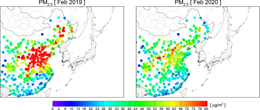
10068                    H. C. Kim et al.: Quantitative assessment of changes in surface particulate matter concentrations

                                                                      from a three-dimensional chemistry model to calculate esti-
                                                                      mated emissions. Since the model simulations with a fixed
                                                                      emission inventory respond to the variations in meteorologi-
                                                                      cal conditions, we can infer the relationship between emis-
                                                                      sions and ambient pollutant concentrations under specific
                                                                      weather conditions. By applying this relationship, we con-
                                                                      vert the changes in observed concentrations into the changes
                                                                      in emissions. Weekly variations, a unique feature of anthro-
                                                                      pogenic emissions, were removed by using a 7 d moving av-
                                                                      erage. The impact of the Chinese spring festival, the biggest
                                                                      traditional holiday celebrating Lunar New Year (LNY), was
                                                                      normalized by rearranging the time series to center on the
                                                                      LNY in each solar year. The LNY alignment was neces-
                                                                      sary to account for the irregular occurrence of the LNY
                                                                      dates. Seven-day moving average filtering was also required
                                                                      to avoid unfair comparisons between different weekdays af-
                                                                      ter the LNY alignment. Otherwise, we may compare differ-
                                                                      ent weekdays for different year (e.g., 2020 LNY on 25 Jan-
                                                                      uary, Saturday, and 2019 LNY is February 5, Tuesday). Fig-
                                                                      ure S4 shows that the 7 d moving average filter smooths but
                                                                      does not significantly change the time-series results. Finally,
                                                                      yearly emission variations were removed by setting a base
                                                                      period (−60 to −10 d before LNY) and calculating relative
                                                                      changes from the average of the base period.
Figure 2. Time series of estimated emissions for (a) NO2 and
                                                                         We followed the data-processing procedures suggested by
(b) PM2.5 using 1332 surface-monitoring sites across China. The
gray lines indicate 2017–2019 variations, with their average in
                                                                      Bae et al. (2020b) for their emissions-updating system (here-
the thick gray line, whereas the red line indicates the 2020 varia-   after BAE2020). First, the observational and modeled data
tion. The blue line indicates the 2020 variations in Hubei Province   were paired and tested, and observation sites with more
(46 sites). BASE is used as the pre-LNY period, and (1) and (2) de-   than 20 % of values missing were discarded. To avoid over-
note the period of maximum impact and the recovery period, re-        weighting dense urban sites, observations occurring within
spectively.                                                           the same model grid cell were averaged. Second, weekly
                                                                      variations were removed using 7 d moving averages, and the
                                                                      impact of the Chinese spring festival was normalized by rear-
inputs. The base model simulations use these 2016 emissions           ranging the time series to center on LNY in each year. Third,
for the entire 2017–2020 modeling period.                             meteorological variations were removed by applying the ra-
                                                                      tio between observed and modeled concentrations. Using a
                                                                      simple linear assumption, observed pollutant concentrations
3     Method
                                                                      were combined with the results of the chemical model to cre-
This section describes the following aspects of the analysis:         ate estimates of actual emissions that are less sensitive to me-
(1) data-processing procedures for analyzing the time series,         teorological variations. Use of the linear assumption in the
(2) emission adjustment procedures to update SO2 and NOx              concentration-to-emission conversion is further discussed in
emissions to near real time, and (3) brute-force modeling pro-        Sect. 4.4 The total estimated emissions, Eest , and their rela-
cedures to estimate Chinese emissions by sector. It should be         tive variations, rEest , were calculated as
noted that the time-series analysis (discussed in Sect. 4.1) uti-                    Cobs (t)
lizes fixed emission inventory (i.e., bottom–up emission in-          Eest (t) = Emod ·       ,                                   (1)
                                                                                    Cmod (t)
ventory) and the emission adjustment experiment (Sect. 4.2)                         Eest (t)
utilizes observation-based top–down emissions. The sectoral           rEest (t) = P                · 100 %,                       (2)
                                                                                    Eest (t)/nbase
emission estimation method is for Sect. 4.3.                                     t=base

3.1    Time-series analysis                                           where C is the daily pollutant concentration; t is days from
                                                                      LNY; base and nbase are the pre-LNY base period (shown in
Four types of variation (meteorological, weekly, yearly, and          Fig. 2) and its number of days, respectively; and Emod is the
the Chinese spring festival) were reduced or accounted for            model emissions. To normalize the yearly changes, a base
in the surface observations, as follows. Meteorological influ-        period (−60 to −10 d before LNY) was set, with relative
ences were reduced by combining surface data with output              changes calculated from the average of that base period (i.e.,

Atmos. Chem. Phys., 21, 10065–10080, 2021                                             https://doi.org/10.5194/acp-21-10065-2021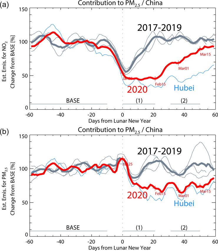
H. C. Kim et al.: Quantitative assessment of changes in surface particulate matter concentrations                              10069

Figure 3. Spatial distribution of the change in estimated NOx emissions from the baseline period (Fig. 2) during the period of maximum
impact (25 January–14 February 2020) and the recovery period (24 February–15 March 2020). Hubei Province is marked in red.

rEest (t)). The impact of the pandemic was inferred by calcu-        β = 1 to update SO2 emissions, and they demonstrated that
lating the difference in estimated emissions between normal          the adjusted emissions effectively reproduced surface SO2
years and 2020. Since the model uses a fixed emission inven-         concentrations over China. Similar approaches were also
tory for each year, Emod cancels out in the comparison.              confirmed to be effective for the NOx emission adjustment
   For the spatial analyses of the data (e.g., Fig. 3), point data   over the same East Asian domain using satellite-based mea-
were converted to area format. Similar to the time-series data       surements of NO2 column densities (Bae et al., 2020a; Chang
processing, the observational and modeled data were paired           et al., 2016).
and tested. Considering the location of each paired data set,           While this simple assumption works practically, we tried
we assigned point data to their corresponding Chinese pre-           to conduct the emission adjustment processing more care-
fecture. By averaging all concentrations in each prefecture,         fully, considering the unprecedented changes in the chemical
we constructed the prefecture-level concentration data set           environment during the pandemic period. We extend the ap-
(for each prefecture polygon), which was then converted into         proach of BAE2020, offering two major enhancements. First,
domain grids using a conservative spatial-regridding tech-           we calculate daily emission adjustment factors to represent
nique. Section 4.4 further discusses the data-processing pro-        the rapid changes in emissions under the pandemic situa-
cedures.                                                             tion. We applied 14 d moving averages to avoid uncertainties
                                                                     caused by insufficient data points day to day. Second, we cal-
3.2   Top–down emission adjustment                                   culated spatial and temporal variations in β and then applied
                                                                     these to the emission adjustment factors. Table 2 compares
For the second analysis (discussed in Sect. 4.2), we updated         the data-processing steps used in this study with those used
major pollutant emissions to a more realistic level and ana-         in BAE2020.
lyzed simulated chemical behaviors. Due to stringent emis-              The β values are calculated as follows. In the real world,
sion control policies by the Chinese government, Chinese             the sensitivity of concentration to changes in emissions is not
anthropogenic emissions have changed dramatically over re-           unique or spatially homogeneous (i.e., β 6 = 1), especially for
cent years. For example, the annual mean surface SO2 con-            NOx emissions and NO2 concentrations. β values for specific
centration across China was 8.4 ppb in 2016 but dropped to           location and time can be calculated if we have two model
less than half of this level (3.7 ppb) in 2020. To incorporate       simulations with different emissions applied. Previous stud-
a realistic change in emissions from 2016 to 2020, we ap-            ies have calculated β values for a model by using changes in
plied observation-based emission adjustment factors to the           concentration caused by a certain amount of perturbed emis-
2016 CREATE emission inventory to reproduce emissions in             sions (e.g., Lamsal et al., 2011, used a 15 % emission pertur-
2020. In general, model emissions can be adjusted based on           bation).
the ratios between observed and modeled surface concentra-              To obtain more realistic β values, we have conducted two
tions:                                                               model simulations: base and adj1 runs. First, the base model
Eadj     Cobs                                                        simulation was conducted using a normal emission inventory,
     =β·      ,                                               (3)    CREATE, which we have introduced previously. The second
Emod     Cmod
                                                                     simulation, adj1 run, was conducted using perturbed emis-
where β is a sensitivity factor in the emission-to-                  sions to estimate how the model responds according to the
concentration conversion. β is close to 1 if less secondary          change in emissions. We adjusted emissions according to the
chemical reactions are involved. BAE2020 assumed a fixed

https://doi.org/10.5194/acp-21-10065-2021                                           Atmos. Chem. Phys., 21, 10065–10080, 2021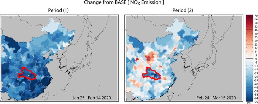
10070 H. C. Kim et al.: Quantitative assessment of changes in surface particulate matter concentrations
Table 2. Comparison of data-processing steps in the emission adjustment methods used in BAE2020 and this study.
Data-processing steps BAE2020 This study
Spatial processing Prefecture-level Prefecture-level
Temporal processing Monthly Daily (14 d moving average)
Emission-to-concentration β =1 Varying
conversion factor (β) (Daily and prefecture-level)
CMAQ simulations 1 (adj1) 2 (adj1 & adj2)
Emissions adjusted SO2 SO2 , NOx
Note: results of “adj1” simulations were used to calculate β values for the “adj2” simulation.
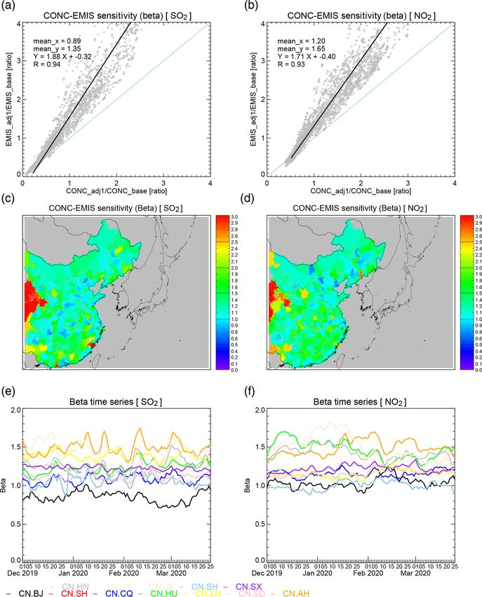
ratio between observed and modeled surface concentrations, 4 Results
so we can reproduce a more realistic chemical environment.
From these two simulations, the base and adj1 runs, we 4.1 Time-series analysis
calculate the emissions-to-concentration sensitivity, β val-
ues, on a specific spatial and temporal scale – for each Chi-
nese prefecture daily. β values are calculated as Reducing meteorological, weekly, and yearly variations, as
well as variations resulting from the Chinese spring festival
[Eadj1 /Ebase ]p,t made the comparison of pandemic-influenced surface obser-
βp,t = , (4)
[Cadj1 /Cbase ]p,t vations to normal conditions more robust and useful. Esti-
mated NOx emissions (Fig. 2) display variations from the
where p and t stand for indices of Chinese prefectures and spring festival season. From 2017–2019, the estimated NOx
specific dates. Using calculated β values for each prefecture emissions demonstrate a clear reduction during the festival
and date, we finally obtain the adjusted emissions for the sec- period (by up to 45 % between −10 and +20 d from LNY).
ond and final simulations: the adj2 run. In 2020, this reduction is slightly greater and continues for
Cobs
longer, implying that the coronavirus outbreak further re-
[Eadj2 ]p,t = βp,t · · Ebase (5) duced traffic in China. The difference between the estimated
Cbase p,t emissions in the 2017–2019 time series and those in the 2020
We further discuss the characteristics of the emissions-to- time series in Fig. 2 reflects the relative significance of the
concentration sensitivity in Sect. 4.4.2. impact of the coronavirus (p < 0.01 for t test of comparison
after LNY).
3.3 Estimation of sectoral contributions Interestingly, the 2020 time series (that is, the combined
effect of the spring festival and the coronavirus) remains
The contributions of emissions from each sector to surface flat from the LNY to 15 February. As both effects likely
PM2.5 concentrations over China were estimated using the overlapped, they appear inseparable during the period. The
brute-force method (BFM), an approach that uses changes maximum impact from the coronavirus seen in the data is
in modeled outputs as a result of perturbed emission inputs a 58 % reduction on 15 February 2020 from the level seen
(Burr and Zhang, 2011). The MIX emission inventory pro- in prior, baseline years (2017–2019). The level of NOx emis-
vides information on five sectors: residential, industry, power sions from 1 to 15 February (close to a 50 % reduction) might
generation, transportation, and agriculture. Sectoral contribu- suggest a floor level for reduced emissions under current
tions were calculated by applying the perturbed emissions for conditions in terms of technology and infrastructure. This
each sector: might have important implications for chemical modeling
(Cbase − C1E,sector )/1E and emission control, perhaps implying a floor for emission
Contr.(sector) = · 100 %, (6) reductions that China can realistically reach under current
Cbase
conditions. The blue line represents a time series from Hubei
where C is the surface PM2.5 concentration and 1E is the only (46 sites), showing, as would be expected, that the im-
ratio of the emission perturbations. A 50 % reduction was pact in Hubei has been more significant and sustained.
chosen to perturb emissions for each individual sector. Frac- The reduced NOx emissions began to increase after
tional contributions of each emission sector were calculated 15 February, almost recovering to their normal level by
compared to the sum of all five emission sector contributions. the end of March 2020. Hence, the impact of the coron-
The application of the BFM to East Asian air quality mod- avirus pandemic on NOx emissions in China lasted almost
els and a discussion of its uncertainties has been presented 2 months. Figure 3 shows the spatial distribution of the esti-
elsewhere (Kim et al., 2017b). mated changes in NOx emissions from the base period to the
Atmos. Chem. Phys., 21, 10065–10080, 2021 https://doi.org/10.5194/acp-21-10065-2021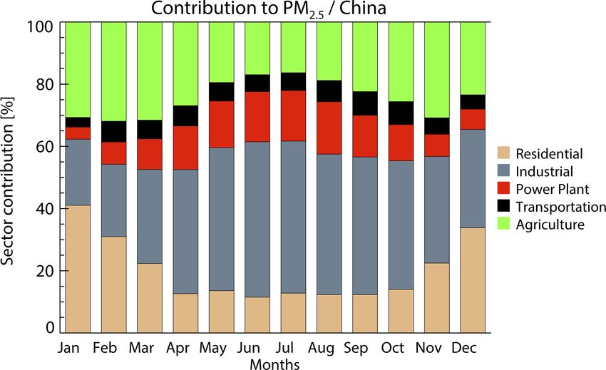
H. C. Kim et al.: Quantitative assessment of changes in surface particulate matter concentrations                           10071

period of maximum impact (25 January–14 February 2020)             4.2   Experiment with updated SO2 and NOx emissions
and the recovery period (24 February – 15 March 2020). Just
after LNY, NOx emissions strongly reduce across China, but         As discussed in Sect. 3.2 above, we used an alternative ap-
their inferred recovery is spatially inhomogeneous. As shown       proach to investigate unidentified PM2.5 emissions, specifi-
in Fig. 3, Hubei Province continued to show a strong reduc-        cally applying more realistic SO2 and NOx emission adjust-
tion (by more than 50 %) compared with the pre-LNY level,          ments. Using this methodology, we repeated CMAQ sim-
even in the recovery phase (period 2). Other regions show          ulations with SO2 and NOx emissions adjusted based on
various patterns in NOx levels compared with previous years.       surface measurements. Daily and prefecture-level emission-
These observations are consistent with space-borne, remote-        adjustment factors were calculated and applied to the base-
sensing measurements from the TROPOMI (Fig. S1). Similar           line emission inventory. The two CMAQ simulations – a
to the surface observations in Fig. 3, the spatial distributions   baseline simulation with the CREATE emission inventory
of NO2 column densities during the period of maximum im-           and an adjustment simulation with updated emissions – were
pact (25 January–14 February) and the recovery period (24          both compared with observations from surface-monitoring
February – 15 March) were generated as changes from the            sites (Fig. 4). Individual site comparisons are also available
baseline period (26 November 2019–15 January 2020).                in Fig. S11.
   The impact of the virus may actually have begun before             For both SO2 and NO2 concentrations, the CMAQ simu-
the spring festival. In normal years (2017–2019), variation        lation with adjusted emissions performed well, reproducing
in estimated pre-LNY baseline period (−60 to −10 d) NOx            observed variations in surface concentrations. It should be
emissions is relatively small because the model uses fixed         noted that the CREATE v2.3 emission inventory we used was
emissions and weekly variations have already been removed.         constructed for 2016 and applied to a 2020 simulation. Be-
However, the estimated emissions in 2020 are relatively low,       fore LNY, simulated NO2 concentrations with both the base-
starting from about 15 d before LNY, and this relative re-         line and adjusted emission inventory agreed well with obser-
duction is more pronounced in Hubei. This suggests that our        vations, implying that there were no significant changes in
baseline period in 2020 already includes a partial coronavirus     the NOx emission level between 2016 and 2020. Near LNY,
impact. If this is true, the impact of the pandemic would be       the baseline NO2 simulations differ significantly from obser-
even stronger than inferred here, as it is based on a year-        vations, while the simulation with adjusted emissions suc-
by-year comparison of concentrations during and after the          cessfully reproduced the huge reductions in the LNY and
typical-year base period.                                          pandemic period. The difference between the baseline and
   Unlike the temporal trend in NOx emissions and their spa-       adjusted simulations almost disappears at the end of March,
tial distribution, a comparison of changes in the PM2.5 level      consistent with the result of the time-series analysis (Fig. 2).
suggests a different story (Fig. 2b). Contrary to NOx emis-        On the other hand, the baseline SO2 simulations greatly over-
sions, PM2.5 concentrations typically show a slight increase       estimate observations by 2 or 3 times, implying that nomi-
near LNY, likely due to increased PM2.5 emissions from fire-       nal, real-world SO2 emissions in 2020 are much smaller than
works, a long-held tradition in China (Kong et al., 2015), and     those reflected in the 2016 emission inventory. By applying
show only a relatively moderate reduction from typical lev-        the top–down adjustment described here, simulations could
els (by 10 %–20 %) over the remainder of the spring festival.      successfully reproduce surface SO2 concentrations, reduc-
Unlike NOx emissions, the case of PM2.5 involves both di-          ing RMSE by 93 % from 9.19 to 0.62 ppb. The updated SO2
rect emissions of particulate matter and gas-to-particle con-      and NOx emission inventories appear to successfully repro-
version of emitted precursors (e.g., SO2 , NOx , NH3 , VOCs –      duce variations in surface PM2.5 concentrations, even after
volatile organic compounds) mediated by atmospheric chem-          the start of LNY celebrations. However, in early February, as
ical transformations. As discussed in the Method section,          the impact of the COVID-19 pandemic became more signifi-
we assume the same approximate relationship for PM2.5 as           cant, the baseline run (with the CREATE emission inventory)
with NOx between the ambient observations and their asso-          does not simulate a sudden drop in PM2.5 observations, while
ciated emissions. This approach suggests that emissions de-        the adjusted emissions run does so.
creased by roughly 30 % from normal levels through the end            A closer look, however, reveals that the real trend in PM2.5
of March to reach 72.7 ± 6.6 % of the 2017–2019 level from         emissions cannot be explained by the change in two major
4 February to 25 March 2020. Interestingly, the pandemic           inorganic aerosol precursors: SO2 and NOx . Figure 5 depicts
does not seem to have significantly affected SO2 emissions         the time series of normalized mean biases (NMBs) of surface
(see Fig. S3), suggesting that the pandemic’s effects on the       PM2.5 concentrations. Before LNY, PM2.5 NMB is mostly
power generation and industrial sectors have been relatively       negative, showing the adjusted emission simulation slightly
small.                                                             underestimates particulate matter. After LNY, PM2.5 NMB
                                                                   changes prominently, showing the simulation clearly overes-
                                                                   timates observations by about 20 % NMB in PM2.5 concen-
                                                                   tration. Before and after LNY, PM2.5 NMB moves by 25.1 %,
                                                                   from −4.1 % to 21.0 %, implying that the model suddenly

https://doi.org/10.5194/acp-21-10065-2021                                        Atmos. Chem. Phys., 21, 10065–10080, 2021
10072 H. C. Kim et al.: Quantitative assessment of changes in surface particulate matter concentrations
Figure 4. Time series and scatterplots of observed and modeled surface concentrations of SO2 , NO2 , and PM2.5 from 1332 Chinese surface-
monitoring sites during the pandemic period. Model simulations using the baseline emission inventory (CREATE) and top–down adjusted
emissions are shown in blue and red, respectively. Observations are represented by gray circles.
overestimates PM2.5 concentrations by 25 % after LNY. In
other words, unknown, non-modeled emissions (that is, non-
SO2 and non-NOx emissions) are clearly reduced enough
during the pandemic period (February and March) to account
for 25 % of total PM2.5 concentration at baseline. This result
is consistent with findings (Sect. 4.1) that changes in SO2
and NOx emissions alone cannot explain the reduced PM2.5
concentrations in March.
4.3 Sectoral contributions to emissions
One remaining question is why the recovery of NOx emis-
sions and unchanged SO2 emissions at the end of March did
not lead to the recovery of PM2.5 , which might be explained
by considering the time-varying emission contribution of
each economic sector. Sensitivity tests using the CMAQ
model reveal that the residential and agricultural sectors are
Figure 5. Time series of surface PM2.5 normalized mean bias dur- most dominant in the early months of the year (Fig. 6), ac-
ing the pandemic period between observed and modeled data with counting for more than 60 % of surface PM2.5 concentration
adjusted emissions (i.e., SO2 and NOx emissions adjusted). Mean over China. As emissions in the residential sector are primar-
NMBs before and after LNY are also marked. Raw, 7 d, and 14 d ily from cooking and heating with anthracite coal and wood,
moving average NMBs are shown in thin, medium-thin, and thick emissions which continue even during a pandemic, one pos-
lines, respectively. sible explanation is that emissions from the agricultural sec-
tor reduced as a result of pandemic-related delays in planting
and fertilizing.
Atmos. Chem. Phys., 21, 10065–10080, 2021 https://doi.org/10.5194/acp-21-10065-2021H. C. Kim et al.: Quantitative assessment of changes in surface particulate matter concentrations 10073
transport, and dispersion, can create large gradients on lo-
cal scales that are likely poorly represented in the WRF
and CMAQ modeling performed here, even as their impor-
tance is somewhat smoothed over regional and nationwide
scales. Observed concentrations of a pollutant are generally
proportional to the emissions associated with that pollutant;
conceptually, a simple linear relationship between emissions
and pollutants is assumed. For the pollutants NO2 and SO2 ,
these are NOx and SO2 emissions, respectively. BAE2020
demonstrated that this concentration-to-emission conversion
method can be used effectively at the Chinese prefecture
level. Discussion of the spatial representativeness of Chi-
nese surface-monitoring data and associated uncertainties
Figure 6. Monthly variations in emission contributions to surface is also presented in BAE2020. For inferring PM2.5 -related
PM2.5 concentrations over China by sector. The contributions from emissions, the analysis is more complicated because PM2.5
the five sectors (residential, industry, power generation, transporta- results from both primary and secondary (precursor) emis-
tion, and agriculture) were estimated using a brute-force perturba- sions. While the pollutant–emissions relation for PM2.5 is
tion method. nonlinear, especially over relatively small spatial and tem-
poral scales, it is still approximately valid over larger geo-
February is the start of the spring-crop planting period in graphical regions and longer time periods.
southern China. The coronavirus outbreak could have im- The validity of the linear assumption was tested through a
pacted both field crops and livestock farms. Inputs, such as model sensitivity analysis. A CMAQ simulation with 50 %
fertilizer and animal feed, have reportedly been scarce as reduced emissions yielded an approximately 50 % reduc-
a result of transportation disruptions, and seasonal workers tion in surface PM2.5 concentrations over most regions in
have reportedly been lacking due to quarantine controls or China (Table S1 in the Supplement). Taken as a whole, sur-
fears (Quanying, 2020; Yu, 2020; Zhang and Xiong, 2020). face PM2.5 concentrations are roughly proportional to over-
Agricultural activities that generate particulate matter, such all emissions. Thus, the simplifying assumption of linearity
as biomass burning to clear debris and the generation of air- appears reasonable for the more complex PM2.5 case, gener-
borne dust during tilling, are reduced in intensity during the ating a time series of estimated pollutant emissions without
pandemic. Reduced NH3 emissions as a result of diminished meteorological variations. Nevertheless, PM2.5 emissions es-
livestock farming activities might also be a factor leading to timated with this analysis are necessarily more uncertain than
lower PM2.5 concentrations. are NOx emissions. Notably, Table S1 also shows that CMAQ
simulations with adjustments in SO2 , NOx , and NH3 individ-
4.4 Further discussions on the methods ually showed disproportionately lower responses, suggest-
ing that surface PM2.5 concentrations are influenced by other
4.4.1 On the data processing of time-series analysis emissions (e.g., elemental carbon and organic carbon emis-
sions) and/or nonlinear processes that likely vary with atmo-
We further discuss data-processing procedures here. Fig- spheric chemistry regime.
ure 7 presents a time series of surface pollutants proceed-
ing through data-processing steps. Even in raw format, NO2 4.4.2 On the emission adjustment experiment
exhibits clear impacts from the pandemic. Impacts on other
pollutants (CO, PM10 , and PM2.5 ), however, are not easily As stated in the methodology section, we further discuss
recognizable until confounding signals are fully removed. In- here the emissions-to-concentration sensitivities (i.e., β).
terpreting SO2 concentration data is particularly illuminat- The β values can be calculated using any two model simu-
ing. While 2020 SO2 concentrations are substantially lower lations based on different emission inputs, by comparing the
than those of previous years, the time series obtained after change in emissions with the change in simulated concentra-
the data processing described here suggests that SO2 emis- tions. Furthermore, if we specifically change the emissions
sions are mostly consistent before and after LNY. That is, according to the ratio of observations and the base model
lower SO2 concentrations in 2020 seem to be a continuation simulation, we further simplify the emission scaling factor
of year-over-year reductions and not a result of the pandemic. as follows.
Note that the various instances of linear assumptions used For this simulation, adj1, if we apply the adjusted emis-
in this analysis should be interpreted with caution espe- sions using the ratio of the observed and modeled concentra-
cially considering its spatiotemporal resolution and chem- tions, the adjusted emissions for the adj1 run, Eadj1 , are
ical characteristics. Variations in emissions and in chem- Cobs
ical and physical processes, including chemical reactions, Eadj1 = · Ebase . (7)
Cbase
https://doi.org/10.5194/acp-21-10065-2021 Atmos. Chem. Phys., 21, 10065–10080, 202110074 H. C. Kim et al.: Quantitative assessment of changes in surface particulate matter concentrations Figure 7. Time series of surface NO2 , SO2 , CO, O3 , PM2.5 , and PM10 concentrations over China following the data-processing procedures step by step. Raw data (left column), data after applying a 7 d moving average and an LNY alignment (middle column), and data after removing meteorological variations and calculating variations from the baseline periods (right column) are all shown. Atmos. Chem. Phys., 21, 10065–10080, 2021 https://doi.org/10.5194/acp-21-10065-2021
H. C. Kim et al.: Quantitative assessment of changes in surface particulate matter concentrations 10075
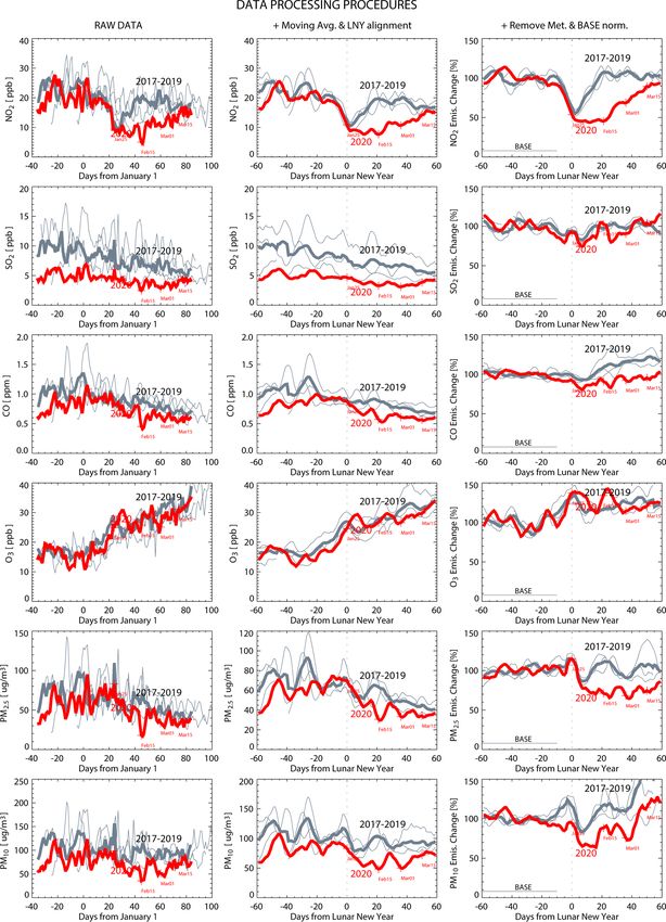
If we apply this to Eq. (4), we can obtain Figure 8 summarizes the characteristics of the β values.
As they are defined as the ratio of the emission change
Eadj1 /Ebase Cobs /Cbase Cobs (i.e., Eadj1 /Ebase ) to the change in concentrations (i.e.,
β= = = . (8)
Cadj1 /Cbase Cadj1 /Cbase Cadj1 Cadj1 /Cbase ), the slopes of the fitted lines in the scatter-
plots describe the emissions-to-concentration sensitivities for
Therefore, the emission adjustment factors in the next sim- SO2 and NO2 (Fig. 8a and b). The histogram of the occur-
ulation (adj2) can be found using Eq. (5): rence of the β values also confirms that for both SO2 and
Cobs
Cobs Cobs
NO2 , the calculated β values are centered slightly over 1
Eadj2 = β · · Ebase = · · Ebase , (9) (mean = 1.42 and median = 1.27 for SO2 and mean = 1.40
Cbase Cadj1 Cbase
and median = 1.26 for NO2 ) (Fig. S13). Figure 8c and d
where adj2 indicates the second and final simulation for the demonstrate the spatial distributions of the β values over Chi-
top–down emission nese territories. Except for a few outside locations, the β val-
h adjustment method.
ues are mostly consistent, around 1. We further investigated
i
Cobs
From here, the Cadj1 term, or β, can be interpreted as an
the temporal variations in the β values by showing the daily
additional
h adjustment
i factor to the original adjustment factor variations in the estimated β values for selected Chinese
in adj1, CCbase
obs
. If the emission modification in adj1 results in provinces (Fig. 8e and f). It is evident that the β values dif-
the same percentage change in concentrations, Cobs /Cadj1 = fer by location, implying that the emissions-to-concentration
1, we do not need the secondary adjustment. If the simulated sensitivities vary for different regions likely due to their
concentration from adj1 is smaller (larger) than the observa- unique chemical and emission environment. However, for
tions, we need to increase (reduce) the amounts of emissions. each location, the β values are mostly consistent over time.
This procedure was applied to create new 2020 emissions of For the practical use of the β values in the emission update
both SO2 and NOx . procedure, we may use region-specific sensitivity parameter-
In most cases, the calculated β values are close to 1 ization since their temporal variations over a specific region
(Fig. S5), implying that the simple assumption β = 1 in are not significant.
BAE2020 remains effective. The β values for NOx emissions To evaluate the emission update approach, the key feature
are slightly higher than those for SO2 emissions over polluted in this study is the validation of PM2.5 concentration. We
areas (Fig. S6), which implies that more secondary reactions used observation-based SO2 and NO2 emission adjustments,
are involved in tropospheric NOx chemistry. and there was no adjustment in the primary PM2.5 emissions,
Both enhancements to the top–down simulations – β val- meaning that the improvement of PM2.5 is achieved through
ues and the daily application of emission adjustment factors – chemical reactions and their balances. The surface concen-
clearly improved the model’s performance, especially in the trations of surface PM2.5 concentrations, especially inorganic
pre-LNY periods. While the monthly emission adjustments aerosols, are formed by secondary reactions, which are deter-
failed to represent the rapid changes in NO2 concentrations mined by the balance of chemical reactions for nitrate, sul-
after 25 January 2020 (Fig. S7), the daily adjustment method fate, and ammonium. The performance of the PM2.5 simu-
successfully modeled these changes (Fig. 4). The general un- lations provides strong evidence that the top–down emission
derestimation of NO2 concentrations was corrected using the adjustment method used in this study is valid and success-
β values (Fig. 4). The improved model performance was con- fully reproduces a realistic chemical environment.
firmed by comparing the spatial distributions and scatterplots Formation efficiency of sulfate aerosols by updating SO2
before and after these adjustments (Figs. S8–S10). Spatial and NOx emission is also very interesting. From Fig. 4, one
distributions of RMSEs of model performances in SO2 , NO2 , may notice that the change in total PM2.5 concentration is
and PM2.5 are also summarized in Fig. S12. not prominent in the pre-pandemic period, even with strong
Understanding the characteristics of the β values in terms reduction in SO2 emissions. Modeled PM speciation com-
of their spatial distribution, temporal variation, and chemical ponents show that the reduced sulfate concentrations were
difference is important for several reasons. In the emission canceled out by the increased nitrate concentrations, due to
update procedure in practice, we can apply the pre-calculated the balance of nonlinear nitrate–sulfate–ammonium chem-
β values from the look-up table if the β values show general istry. Nitrate is the most dominant component of PM2.5 dur-
consistency according to their location, time, and chemical ing the wintertime (contributing ∼ 50 % while sulfate con-
component. For the emission control policy, the β values pro- tributes 14 %), and the sudden drop of PM2.5 concentrations
vide valuable information on the efficiency of emission con- during the pandemic is mostly driven by the change in nitrate
trol because they suggest how effectively pollutant concen- concentrations. This result implies an important message to
trations can be removed given the amount of emission control emission control policy, suggesting that both SO2 and NOx
by the government. emission reductions will be required to achieve better emis-
sion reduction efficiency.
https://doi.org/10.5194/acp-21-10065-2021 Atmos. Chem. Phys., 21, 10065–10080, 202110076 H. C. Kim et al.: Quantitative assessment of changes in surface particulate matter concentrations
Figure 8. Calculation of the concentration-to-emissions sensitivities (β) for the emission adjustment experiment of SO2 (left column) and
NO2 (right column). The β values are obtained as the ratio of the emission change (i.e., Emis_adj / Emis_base) to the change in concentrations
(i.e., Conc_adj1/Conc_base), which is also consistent with the slope in the scatterplot (a, b). Spatial variations in the average concentration-
to-emissions sensitivities (β) during January to March 2020 over China (c, d). The temporal variations in the β values for selected Chinese
provinces are shown in the lower panel (e, f). (BJ: Beijing; SH: Shanghai; CQ: Chongqing; HU: Hubei; SD: Shandong; AH: Anhui; HN:
Hunan; JS: Jiangsu; SX: Shanxi).
5 Summary removed four types of variation (meteorological, weekly,
yearly, and the LNY) to isolate impacts of coronavirus pan-
demic from observed surface pollutant concentrations. A
We investigated changes in observed surface pollutant con-
chemistry model simulation with fixed emission inventory
centrations and precursor emissions over China and in-
was used to remove meteorological variations. The analy-
ferred changes in human activity as a result of the coro-
sis has shown that NOx emissions across China recovered
navirus pandemic. Three analyses were conducted: (1) a
to almost normal levels 2 months after LNY. However, con-
time-series analysis, (2) an emission adjustment experiment,
sidering the estimated changes in emissions associated with
and (3) sectoral emission contribution estimations. First, we
Atmos. Chem. Phys., 21, 10065–10080, 2021 https://doi.org/10.5194/acp-21-10065-2021H. C. Kim et al.: Quantitative assessment of changes in surface particulate matter concentrations 10077
PM2.5 , some emissions remain missing, as of the end of Competing interests. The authors declare that they have no conflict
March 2020, compared with normal years. Second, an al- of interest.
ternative modeling approach using updated real-time SO2
and NOx emissions also suggested that about 25 % of PM2.5
emissions are likely missing from the period. Third, impacts Disclaimer. The scientific results and conclusions, as well as any
of sectoral emissions were presented to infer the role poten- views or opinions expressed herein, are those of the author(s) and
tial missing emissions or activities. do not necessarily reflect the views of NOAA or the Department of
Commerce.
The surface observations of pollutants and inferred pre-
cursor emissions across China suggest that the country is re-
covering, as evidenced by the apparent resumption of near-
Financial support. This research was supported by the National
normal transportation-related emissions. The pandemic ap- Air Emission Inventory and Research Center (NAIR), South Ko-
pears not to have strongly affected the industrial sector; con- rea. Dasom Lee and Jin-Ho Yoon were supported by the Na-
tinued depression in estimated PM2.5 -associated emissions tional Research Foundation of Korea under the grant NRF-
may be due to effects on the agricultural sector. If the sus- 2021R1A2C1011827.
tained reduction in PM2.5 is due to reduced activity in the
agricultural sector, agricultural production could be affected,
at least in the short term. This could hold important im- Review statement. This paper was edited by James Allan and re-
plications for China’s path to recovery and, potentially, for viewed by five anonymous referees.
broader parts of the world if similar types of agricultural im-
pacts occur elsewhere.
The data analysis approach used here has attempted to iso-
late the ambient data signal due to the coronavirus from other References
sources of variation. The apparent difference between the re-
covery timelines for NO2 and PM2.5 suggests that estimat- Bae, C., Kim, H. C., Kim, B.-U., and Kim, S.: Surface
ing NOx emissions alone is insufficient to draw conclusions ozone response to satellite-constrained SO2 emission adjust-
about the overall recovery of the Chinese economy. Overall, ments and its implications, Environ. Pollut., 258, 113469,
https://doi.org/10.1016/j.envpol.2019.113469, 2020a.
changes in concentrations of atmospheric pollutants can pro-
Bae, C., Kim, H. C., Kim, B.-U., Kim, Y., Woo, J.-H., and Kim, S.:
vide useful information about the spatial and temporal eco-
Updating Chinese SO2 emissions with surface observations for
nomic impacts of the coronavirus pandemic, a serious global regional air-quality modeling over East Asia, Atmos. Environ.,
issue. 228, 117416, https://doi.org/10.1016/j.atmosenv.2020.117416,
2020b.
Bao, R. and Zhang, A.: Does lockdown reduce air pollution? Evi-
Code availability. WRF and CMAQ codes are available at https: dence from 44 cities in northern China, Sci. Total Environ., 731,
//www2.mmm.ucar.edu/wrf/users/download/get_sources.html (last 139052, https://doi.org/10.1016/j.scitotenv.2020.139052, 2020.
access: 25 June 2021) (WRF, 2021) and https://github.com/USEPA/ Beirle, S., Boersma, K. F., Platt, U., Lawrence, M. G., and
CMAQ/tree/4.7.1 (last access: 25 June 2021) (Github, 2021), re- Wagner, T.: Megacity Emissions and Lifetimes of Nitro-
spectively. gen Oxides Probed from Space, Science, 333, 1737–1739,
https://doi.org/10.1126/science.1207824, 2011.
Binkowski, F. S. and Roselle, S. J.: Models-3 Community Mul-
Data availability. CNEMC data are available at http://www.pm25. tiscale Air Quality (CMAQ) model aerosol component 1.
in (last access: 25 June 2021) (CNEMC, 2021). TROPOMI data Model description, J. Geophys. Res., 108, 2001JD001409,
are available at http://tropomi.gesdisc.eosdis.nasa.gov (last access: https://doi.org/10.1029/2001JD001409, 2003.
25 June 2021) (NASA GES DISC, 2021). Burr, M. J. and Zhang, Y.: Source apportionment of fine particulate
matter over the Eastern U. S. Part I: source sensitivity simulations
using CMAQ with the Brute Force method, Atmos. Pollut. Res.,
Supplement. The supplement related to this article is available on- 2, 300–317, https://doi.org/10.5094/APR.2011.036, 2011.
line at: https://doi.org/10.5194/acp-21-10065-2021-supplement. Byun, D. and Schere, K. L.: Review of the Governing
Equations, Computational Algorithms, and Other Compo-
nents of the Models-3 Community Multiscale Air Qual-
ity (CMAQ) Modeling System, Appl. Mech. Rev., 59, 51–77,
Author contributions. HCK and SK conceived the study. HCK and
https://doi.org/10.1115/1.2128636, 2006.
MC prepared the paper. SK, CB, MB, and EK conducted the model
Carter, W. P. L.: The SAPRC-99 Chemical Mechanism and Up-
simulation. Critical review, commentary, and editing of the written
dated VOC Reactivity Scales, available at: http://www.cert.ucr.
work were done by DL, RS, BUK, JHY, and AS. All authors gave
edu/~carter/reactdat.htm (last access: 25 June 2021), 2003.
approval to the final version of the paper.
Chang, C.-Y., Faust, E., Hou, X., Lee, P., Kim, H. C.,
Hedquist, B. C., and Liao, K.-J.: Investigating ambient ozone
formation regimes in neighboring cities of shale plays in
https://doi.org/10.5194/acp-21-10065-2021 Atmos. Chem. Phys., 21, 10065–10080, 202110078 H. C. Kim et al.: Quantitative assessment of changes in surface particulate matter concentrations the Northeast United States using photochemical model- Enhanced secondary pollution offset reduction of primary emis- ing and satellite retrievals, Atmos. Environ., 142, 152–170, sions during COVID-19 lockdown in China, Natl. Sci. Rev., 8, https://doi.org/10.1016/j.atmosenv.2016.06.058, 2016. nwaa137, https://doi.org/10.1093/nsr/nwaa137, 2021. Chang, J. S., Brost, R. A., Isaksen, I. S. A., Madronich, Jang, Y., Lee, Y., Kim, J., Kim, Y., and Woo, J.-H.: Im- S., Middleton, P., Stockwell, W. R., and Walcek, C. J.: provement China Point Source for Improving Bottom-Up A three-dimensional Eulerian acid deposition model: Physi- Emission Inventory, Asia-Pac. J. Atmos. Sci., 56, 107–118, cal concepts and formulation, J. Geophys. Res., 92, 14681, https://doi.org/10.1007/s13143-019-00115-y, 2020. https://doi.org/10.1029/JD092iD12p14681, 1987. Kain, J. S.: The Kain–Fritsch Convective Pa- Chauhan, A. and Singh, R. P.: Decline in PM2.5 con- rameterization: An Update, J. Appl. Meteo- centrations over major cities around the world asso- rol., 43, 170–181, https://doi.org/10.1175/1520- ciated with COVID-19, Environ. Res., 187, 109634, 0450(2004)0432.0.CO;2, 2004. https://doi.org/10.1016/j.envres.2020.109634, 2020. Kang, Y.-H., You, S., Bae, M., Kim, E., Son, K., Bae, C., Chen, F. and Dudhia, J.: Coupling an Advanced Land Surface– Kim, Y., Kim, B.-U., Kim, H. C., and Kim, S.: The im- Hydrology Model with the Penn State–NCAR MM5 Mod- pacts of COVID-19, meteorology, and emission control poli- eling System. Part I: Model Implementation and Sensitivity, cies on PM2.5 drops in Northeast Asia, Sci. Rep., 10, 22112, Mon. Weather Rev., 129, 569–585, https://doi.org/10.1175/1520- https://doi.org/10.1038/s41598-020-79088-2, 2020. 0493(2001)1292.0.CO;2, 2001. Kim, H., Lee, S.-M., Chai, T., Ngan, F., Pan, L., and Lee, CNEMC – China National Environmental Monitoring Center: http: P.: A Conservative Downscaling of Satellite-Detected //www.pm25.in, last access: 25 June 2021. Chemical Compositions: NO2 Column Densities of OMI, Emery, C., Liu, Z., Russell, A. G., Odman, M. T., Yarwood, G., and GOME-2, and CMAQ, Remote Sens.-Basel, 10, 1001, Kumar, N.: Recommendations on statistics and benchmarks to https://doi.org/10.3390/rs10071001, 2018. assess photochemical model performance, J. Air Waste Manage., Kim, H. C., Lee, P., Judd, L., Pan, L., and Lefer, B.: OMI NO2 67, 582–598, https://doi.org/10.1080/10962247.2016.1265027, column densities over North American urban cities: the effect of 2017. satellite footprint resolution, Geosci. Model Dev., 9, 1111–1123, Eskes, H., van Geffen, J., Boersma, K. F., Eichmann, K.- https://doi.org/10.5194/gmd-9-1111-2016, 2016. U., Apituley, A., Pedergnana, M., Sneep, M., Veefkind, Kim, H. C., Kim, S., Kim, B.-U., Jin, C.-S., Hong, S., Park, P. J., and Loyola, D.: Sentinel-5 precursor/TROPOMI R., Son, S.-W., Bae, C., Bae, M., Song, C.-K., and Stein, Level 2 Product User Manual Nitrogen dioxide, avail- A.: Recent increase of surface particulate matter concentrations able at: https://sentinel.esa.int/documents/247904/2474726/ in the Seoul Metropolitan Area, Korea, Sci. Rep., 7, 4710, Sentinel-5P-Level-2-Product-User-Manual-Nitrogen-Dioxide https://doi.org/10.1038/s41598-017-05092-8, 2017a. (last access: 25 June 2021), 2019. Kim, H. C., Kim, E., Bae, C., Cho, J. H., Kim, B.-U., and Kim, Georgoulias, A. K., van der A, R. J., Stammes, P., Boersma, S.: Regional contributions to particulate matter concentration K. F., and Eskes, H. J.: Trends and trend reversal detection in the Seoul metropolitan area, South Korea: seasonal variation in 2 decades of tropospheric NO2 satellite observations, At- and sensitivity to meteorology and emissions inventory, Atmos. mos. Chem. Phys., 19, 6269–6294, https://doi.org/10.5194/acp- Chem. Phys., 17, 10315–10332, https://doi.org/10.5194/acp-17- 19-6269-2019, 2019. 10315-2017, 2017b. Github: USEPA/CMAQ, available at: https://github.com/USEPA/ Kim, H. C., Kim, S., Lee, S. H., Kim, B. U., and Lee, CMAQ/tree/4.7.1, last access: 25 June 2021. P.: Fine-Scale Columnar and Surface NOx Concentra- He, G., Pan, Y., and Tanaka, T.: The short-term impacts of COVID- tions over South Korea: Comparison of Surface Moni- 19 lockdown on urban air pollution in China, Nature Sustain- tors, TROPOMI, CMAQ and CAPSS, Inventory, 11, 101, ability, 3, 1005–1011, https://doi.org/10.1038/s41893-020-0581- https://doi.org/10.3390/atmos11010101, 2020. y, 2020. Kong, S. F., Li, L., Li, X. X., Yin, Y., Chen, K., Liu, D. T., Yuan, Hertel, O., Berkowicz, R., Christensen, J., and Hov, Ø.: Test L., Zhang, Y. J., Shan, Y. P., and Ji, Y. Q.: The impacts of of two numerical schemes for use in atmospheric transport- firework burning at the Chinese Spring Festival on air quality: chemistry models, Atmos. Environ. A-Gen., 27, 2591–2611, insights of tracers, source evolution and aging processes, At- https://doi.org/10.1016/0960-1686(93)90032-T, 1993. mos. Chem. Phys., 15, 2167–2184, https://doi.org/10.5194/acp- Hong, S.-Y., Dudhia, J., and Chen, S.-H.: A Revised Ap- 15-2167-2015, 2015. proach to Ice Microphysical Processes for the Bulk Lamsal, L. N., Martin, R. V., Padmanabhan, A., van Donke- Parameterization of Clouds and Precipitation, Mon. laar, A., Zhang, Q., Sioris, C. E., Chance, K., Kurosu, Weather Rev., 132, 103–120, https://doi.org/10.1175/1520- T. P., and Newchurch, M. J.: Application of satellite ob- 0493(2004)1322.0.CO;2, 2004. servations for timely updates to global anthropogenic NOx Hong, S.-Y., Noh, Y., and Dudhia, J.: A new vertical dif- emission inventories, Geophys. Res. Lett., 38, L05810, fusion package with an explicit treatment of entrain- https://doi.org/10.1029/2010GL046476, 2011. ment processes, Mon. Weather Rev., 134, 2318–2341, Li, J., Nagashima, T., Kong, L., Ge, B., Yamaji, K., Fu, J. S., https://doi.org/10.1175/MWR3199.1, 2006. Wang, X., Fan, Q., Itahashi, S., Lee, H.-J., Kim, C.-H., Lin, C.- Huang, X., Ding, A., Gao, J., Zheng, B., Zhou, D., Qi, X., Tang, Y., Zhang, M., Tao, Z., Kajino, M., Liao, H., Li, M., Woo, J.- R., Wang, J., Ren, C., Nie, W., Chi, X., Xu, Z., Chen, L., Li, Y., H., Kurokawa, J., Wang, Z., Wu, Q., Akimoto, H., Carmichael, Che, F., Pang, N., Wang, H., Tong, D., Qin, W., Cheng, W., Liu, G. R., and Wang, Z.: Model evaluation and intercomparison of W., Fu, Q., Liu, B., Chai, F., Davis, S. J., Zhang, Q., and He, K.: surface-level ozone and relevant species in East Asia in the con- Atmos. Chem. Phys., 21, 10065–10080, 2021 https://doi.org/10.5194/acp-21-10065-2021
You can also read