Phase-sensitive tipping: How cyclic ecosystems respond to contemporary climate - arXiv.org
←
→
Page content transcription
If your browser does not render page correctly, please read the page content below
Phase-sensitive tipping: How cyclic ecosystems respond to
                                                               contemporary climate
                                                       Hassan Alkhayuon∗, Rebecca C. Tyson†, and Sebastian Wieczorek∗
                                                                                            January 2021

                                                                                               Abstract
                                                      We identify the phase of a cycle as a new critical factor for tipping points (critical
arXiv:2101.12107v1 [math.DS] 28 Jan 2021

                                                  transitions) in cyclic systems subject to time-varying external conditions. As an example,
                                                  we consider how contemporary climate variability induces tipping from a predator-prey
                                                  cycle to extinction in two paradigmatic predator-prey models with an Allee effect. Our
                                                  analysis of these examples uncovers a counter-intuitive behaviour, which we call phase-
                                                  sensitive tipping or P-tipping, where tipping to extinction occurs only from certain phases
                                                  of the cycle. To explain this behaviour, we combine global dynamics with set theory and
                                                  introduce the concept of partial basin instability for limit cycles. This concept provides a
                                                  general framework to analyse and identify sufficient criteria for the occurrence of phase-
                                                  sensitive tipping in externally forced systems.

                                           1      Introduction
                                           Tipping points or critical transitions are fascinating nonlinear phenomena that are known to
                                           occur in complex systems subject to changing external conditions or external inputs. They are
                                           ubiquitous in nature and, in layman’s terms, can be described as large, sudden, and unexpected
                                           changes in the state of the system triggered by small or slow changes in the external inputs [1, 2].
                                           Owing to potentially catastrophic and irreversible changes associated with tipping points, it is
                                           important to identify and understand the underlying dynamical mechanisms that enable such
                                           transitions. Recent work on tipping from base states that are stationary (attracting equilibria)
                                           for fixed external conditions, but change their position or stability as the external conditions vary
                                           over time, identified three generic tipping mechanisms [3]:
                                                • Bifurcation-induced tipping or B-tipping occurs when the external input passes through a
                                                  dangerous bifurcation of the base state, at which point the base state disappears or turns
                                                  unstable, forcing the system to move to a different state [4, 5, 6].
                                                • Rate-induced tipping or R-tipping occurs when the external input varies too fast, so the
                                                  system deviates too far from the moving base state and crosses some tipping threshold [7,
                                                  8, 9, 10, 11, 12], e.g. into the domain of attraction of a different state [13, 14, 15, 16, 17, 18].
                                                  The special case of delta-kick external input is referred to as shock-tipping or S-tipping [19].
                                                  In contrast to B-tipping, R-tipping need not involve any bifurcations of the base state.
                                                • Noise-induced tipping or N-tipping occurs when external random fluctuations drive the
                                                  system too far from the base state and past some tipping threshold [20], e.g. into the
                                                  domain of attraction of a different state [21, 22, 23, 24].
                                               Many complex systems have non-stationary base states, meaning that these systems exhibit
                                           regular or irregular self-sustained oscillations for fixed external inputs [25, 26, 27, 28, 29, 30, 31,
                                           32]. This opens the possibility for other generic tipping mechanisms when the external inputs
                                           vary over time. In this paper, we focus on tipping from the next most complicated base state, a
                                           periodic state (attracting limit cycle), and identify a new tipping mechanism:
                                               ∗ University   College Cork, School of Mathematical Sciences, Western Road, Cork, T12 XF62, Ireland
                                               † Department    of Mathematics and Statistics, University of British Columbia Okanagan, Kelowna, BC, Canada

                                                                                                    1
• Phase-sensitive tipping or P-tipping occurs when a too fast change or random fluctuations
     in the external input cause the system to tip to a different state, but only from certain
     phases of the base state. In other words, the system has to be in the right phases to tip,
     whereas no tipping occurs from other phases.
    The concept of P-tipping naturally extends to more complicated quasiperiodic (attracting
tori) and chaotic (strange attractors) base states and, in a certain sense, unifies the notions of
R-tipping, S-tipping and N-tipping. A simple intuitive picture is that external inputs can trigger
the system past some tipping threshold, but only from a certain part of the base state. Thus, P-
tipping can also be interpreted as partial tipping. Indeed, examples of P-tipping with smoothly
changing external inputs include the recently studied “partial R-tipping” from periodic base
states [27], and probabilistic tipping from chaotic base states [29]. Furthermore, P-tipping offers
new insight into classical phenomena such as stochastic resonance [21, 33, 34], where noise-induced
transitions between coexisting non-stationary states occur (predominantly) from certain phases
of these states and at an optimal noise strength. Other examples of P-tipping due to random
fluctuations include “state-dependent vulnerability of synchronization” in complex networks [35],
and “phase-sensitive excitability” from periodic states [20], which can be interpreted as partial
N-tipping.
    Here, we construct a general mathematical framework to analyse irreversible P-tipping from
periodic base states. By “irreversible” we mean that the system leaves the stable base state and ap-
proaches a different state in the long-term. The framework allows us to explain counter-intuitive
properties, identify the underlying dynamical mechanism, and give easily testable criteria for the
occurrence of P-tipping. Furthermore, motivated by growing evidence that tipping points in the
Earth system could be more likely than was thought [2, 36, 37], we show that P-tipping could oc-
cur in real ecosystems subject to contemporary climate change. To be more specific, we uncover
robust P-tipping from cyclic coexistence of species to extinction due to climate-induced decline
in resources in two paradigmatic predator-prey models with an Allee effect: the Rosenzweig-
McArthur model [38] and the May (or Leslie-Gower-May) model [39]. Both models have been
used to study predator-prey interactions in a number of natural systems [40, 41, 42]. Here, we use
realistic parameter values for the Canada lynx and snowshoe hare system [43, 44], together with
real climate records from various communities in the boreal and deciduous-boreal forest [45].
    The nature of predator-prey interactions often leads to regular, high amplitude, multi-annual
cycles [46]. Consumer-resource and host-parasitoid interactions are similar, and also often lead
to dramatic cycles [47]. In insects, cyclic outbreaks can be a matter of deep economic concern,
as the sudden increase in defoliating insects leads to significant crop damage [48]. In the boreal
forest, one of the most famous predator-prey cycles is that of the Canada lynx and snowshoe
hare [47]. The Canada lynx is endangered in parts of its southern range, and the snowshoe hare is
a keystone species in the north, relied upon by almost all of the mammalian and avian predators
there [49]. These examples illustrate the ubiquitous nature of cyclic predator-prey interactions,
and their significant economic and environmental importance. Their persistence in the presence
of climate change is thus a pressing issue.
    Anthropogenic and environmental factors are subjecting cyclic predator-prey systems to ex-
ternal forcing which, through climate change, is being altered dramatically in both spatial and
time-dependent ways [41, 50, 51, 52, 53, 54]. In addition to long-term changes due to global
warming, there is a growing interest in changes in climate variability on year-to-decade timescales,
owing to its more imminent impacts [55]. In particular, increased variability of short-term cli-
matic events manifests itself as, for example, larger hurricanes, hotter heatwaves, and more severe
floods [56, 57, 58, 59, 60, 61, 53, 62, 63]. It is unknown how cyclic predator-prey systems will
interact with these changes in climate variability.
    Beyond ecology, oscillatory predator-prey interactions play an important role in finance and
economics [64, 65]. Thus, our work may also be relevant for understanding economies in de-
veloping countries [66]. Such economies are non-stationary by nature, and it may well be that
developing countries have only short phases in their development, or narrow windows of oppor-
tunity, during which external investments can induce transitions from poverty to wealth.
    This paper is organized as follows. In Section 2, we introduce the Rosenzweig-MacArthur and
the May models, define phase for the predator-prey cycles, and describe the random processes
used to model climatic variability. In Section 3, Monte Carlo simulations of the predator-prey
models reveal counter-intuitive properties of P-tipping and highlight the key differences from

                                                 2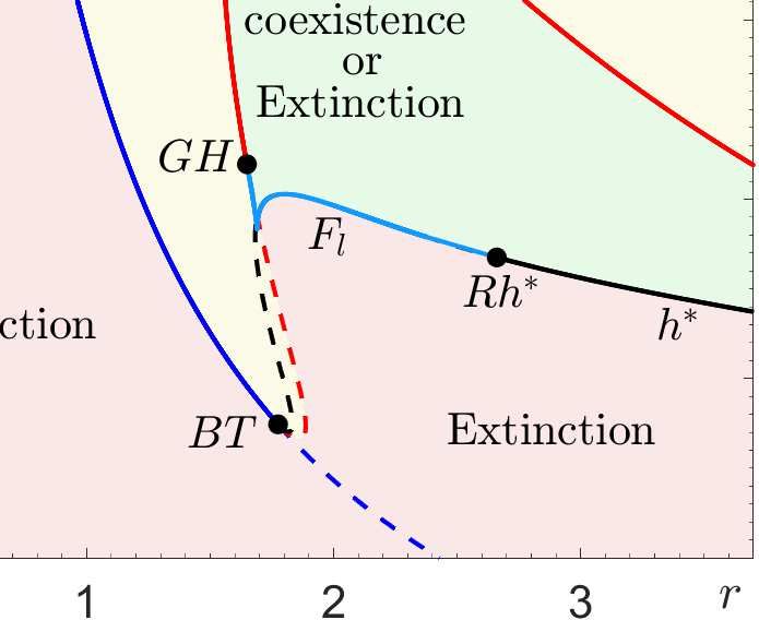
15

                                                    -2
    10

     5                                              -3

     0                                              -4
         0          1            2                       1         2             3

Figure 1: One-parameter bifurcation diagrams with different but fixed-in-time r for (a) the
autonomous RMA frozen model (1) and (b) the autonomous May frozen model (3). The other
parameter values are given in Appendix B, Table 1.

B-tipping. In Section 4, we present a geometric framework for P-tipping and define the concept
of partial basin instability for attracting limit cycles. In Section 5, we produce two-parameter
bifurcation diagrams for the autonomous predator-prey frozen systems with fixed-in-time external
inputs, identify bistability between predator-prey cycles and extinction, and reveal parameter
regions of partial basin instability - these cannot be captured by classical bifurcation analysis
but are essential for understanding P-tipping. Finally, we show that partial basin instability
explains and gives testable criteria for the occurrence of P-tipping. We summarise our results in
Section 6.

2        Oscillatory predator-prey models with varying climate.
To introduce the setting of the paper, we begin with the two predator-prey models.

2.1          The Rosenzweig-MacArthur Model
The Rosenzweig-MacArthur (RMA) model [38, 9] describes the time evolution of interacting
predator P and prey N populations [67]:

                                         c        N −µ     αN P
                      Ṅ = r(t) N 1 −        N           −      ,
                                        r(t)      ν+N      β+N
                                                                                     (1)
                              αN P
                       Ṗ = χ        − δP.
                              β+N

In the prey equation, −r(t)µ/ν is the low-density prey growth rate, cµ/ν quantifies the nonlinear
prey birth rate, the term (N − µ)/(ν + N ) gives rise to the strong Allee effect that accounts for
negative prey growth rate at low prey population density, α is the saturation predator kill rate,
and β is the predator kill half-saturation constant. The ratio r(t)/c is often referred to as the
carrying capacity of the ecosystem. It is the maximum prey population that can be sustained
by the environment in the absence of predators [44]. In the predator equation, χ represents the
prey-to-predator conversion rate, and δ is the predator mortality rate. Realistic parameter values,
estimated from the Canada lynx and snowshoe hare data [44, 43], can be found in Appendix B,
Table 1.
    As we explain in Sec. 22.4, r(t) is a piecewise constant function of time that describes the
varying climate. This choice makes the nonautonomous system (1) piecewise autonomous in the
sense that it behaves like an autonomous system over finite time intervals. Therefore, much

                                                3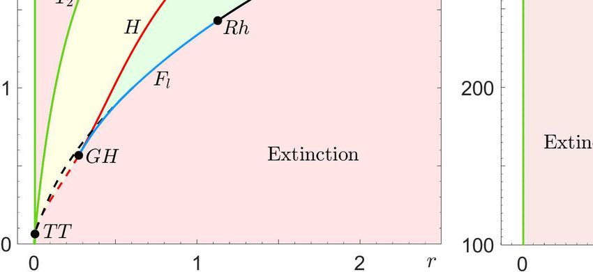
can be understood about the behaviour of the nonautonomous system (1) by looking at the
autonomous frozen system with different but fixed-in-time values of r.
    The RMA frozen system can have at most four stationary states (equilibria), which are
derived by setting Ṅ = Ṗ = 0 in (1). In addition to the extinction equilibrium e0 , which is stable
for r > 0, there is a prey-only equilibrium e1 (r), the Allee equilibrium e2 , and the coexistence
equilibrium e3 (r), whose stability depends on r and other system parameters:

                   e0 = (0, 0), e1 (r) = (r/c, 0), e2 = (µ, 0), e3 (r) = (N3 , P3 (r)).                (2)

In the above, we include the argument (r) when an equilibrium’s position depends on r. The
prey and predator densities of the coexistence equilibrium e3 (r) are given by:

                      δβ                     r    c  (β + N3 )(N3 − µ)
              N3 =          ≥ 0 and P3 (r) =    1 − N3                   ≥ 0.
                     χα − δ                  α     r        ν + N3
    The one-parameter bifurcation diagram of the RMA frozen system in Fig. 1(a) reveals various
bifurcations and bistability, which are discussed in detail in Sec. 55.1. Most importantly, as r is
increased, the coexistence equilibrium e3 (r) undergoes a supercritical Hopf bifurcation H, which
makes the equilibrium unstable and produces a stable limit cycle Γ(r). The cycle corresponds to
oscillatory coexistence of predator and prey and is the main focus of this study. As r is increased
even further, Γ(r) disappears in a dangerous heteroclinic bifurcation h at r = rh , giving rise to a
discontinuity in the branch of coexistence attractors. Past rh , the only attractor is the extinction
equilibrium e0 .

2.2    The May Model
To show that phase-sensitive tipping is ubiquitous in predator-prey interactions, we also consider
another paradigmatic predator-prey model, the May model [39, 44]:

                                           c  N −µ            αN P
                          Ṅ = r(t) N 1 − N                 −         ,
                                            r       ν+N        β+N
                                                                                             (3)
                                           qP
                          Ṗ = sP 1 −             .
                                         N +
This model has the same equation for the prey population density N as the RMA model, but
differs in the equation for the predator population density P . Specifically, s is the low-density
predator growth rate and  is introduced to allow prey extinction. In other words, this model
assumes that the predator must have access to other prey which allow it to survive at a low
density /q in the absence of the primary prey N . The parameter q approximates the minimum
prey-to-predator biomass ratio that allows predator population growth, and Table 1 in Appendix
B contains realistic parameter values, estimated from Canada lynx and snowshoe hare data
[44, 43].
    The May frozen system can have at most five stationary solutions (equilibria), which are
derived by setting Ṅ = Ṗ = 0 in (3). In addition to the extinction equilibrium e0 , which is
always stable, there is a prey-only equilibrium e1 (r), the Allee equilibrium e2 , and two coexistence
equilibria e3 (r) and e4 (r), whose stability depends on the system parameters

 e0 = (0, /q), e1 (r) = (r/c, 0), e2 = (µ, 0), e3 (r) = (N3 (r), P3 (r)) , e4 (r) = (N4 (r), P4 (r)) . (4)

In the above, we include the argument (r) when an equilibrium’s position depends on r. The
prey population densities of the coexistence equilibria e3 (r) and e4 (r) are the two non-negative
roots, denoted N3 (r) and N4 (r) respectively, of the third degree polynomial

                    r    α                 r(β − µ) α(ν + )               rβµ αν
    N3 − µ − β + −           N 2 − βµ +              −             N+          +        = 0,   (5)
                    c cq                        c          cq               c      cq
and the corresponding predator population densities are given by
                                                Ni (r) +
                                     Pi (r) =              , i = 3, 4.
                                                     q

                                                     4
15
                                                      20

                                                      10
   5

                                                       0
       0            5             10                       0           5            10

Figure 2: Phase portraits showing the (green) predator-prey limit cycles Γ(r) together with their
phases ϕγ and basin boundaries θ(r) in (a) the autonomous RMA frozen model (1) with r = 2.47
and (b) the autonomous May frozen model (3) with r = 3.3. The other parameter values are
given in Appendix B, Table 1. Schematic phase portraits depicting all equilibria and invariant
manifolds are shown in Appendix B, Fig. 10.

    The one-parameter bifurcation diagram of the May frozen system in Fig. 1(b) reveals different
bifurcations and bistability. Most importantly, as r is increased, the coexistence equilibrium e3 (r)
gives rise to a stable limit cycle Γ(r) via a safe supercritical Hopf bifurcation, denoted H1 . The
cycle exists for a range of r, and disappears in a reverse supercritical Hopf bifurcation, denoted
H2 , for larger r.

2.3    Phase of the cycle
To depict phase-sensitive tipping, we characterise each point on a limit cycle by its unique phase.
In the two-dimensional phase space of the autonomous predator-prey frozen systems (1) and (3),
the stable limit cycle Γ(r) makes a simple rotation about the coexistence equilibrium e3 (r). We
take advantage of this fact and assign a unique phase ϕγ ∈ [−π, π) to every point γ = (Nγ , Pγ )
on the limit cycle using a polar coordinate system anchored in e3 (r) = (N3 (r), P3 (r)):

                                           −1     3 Pγ − P3
                                  ϕγ = tan      10             .                                (6)
                                                    Nγ − N3

In other words, phase of the cycle is the angle measured counter-clockwise from the horizontal
half line that extends from e3 (r) in the direction of increasing N , as is shown in Fig. 2. Since the
values of P (t) for the limit cycles in systems (1) and (3) are three orders of magnitude smaller
than the values of N (t), the ensuing distribution of ϕγ along Γ(r) is highly non-uniform. To
address this issue and achieve a uniform distribution of ϕγ , we include the factor of 103 in (6).
We use the same definition to assign a phase to trajectories near the limit cycle.

2.4    Climate variability
Climate variability here refers to changes in the state of the climate occurring on year-to-decade
time scales. We model this process by allowing r(t), and thus the carrying capacity of the
ecosystem, vary over time. This variation can be interpreted as climate-induced changes in the
availability of resources or in the quality of habitat. Seasonal modelling studies often assume
sinusoidal variation in climate parameters [68, 69, 70, 71], but many key climate variables vary
much more abruptly [41]. Since our unit of time is years, rather than months, we focus on abrupt
changes in climate.

                                                  5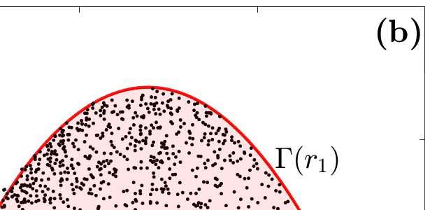
Guided by the the approach proposed in [45], we construct a piecewise constant r(t) using two
random processes; see Fig. 3(a). First, we assume the amplitude of r(t) is a random variable with
a continuous uniform probability distribution on a closed interval [r2 , r1 ]. Second, we assume the
number of consecutive years ` during which the amplitude of r(t) remains constant is a random
variable with a discrete probability distribution known as the geometric distribution1

                                       g(`) = Pr(x = `) = (1 − ρ)` ρ,                                         (7)

where ` ∈ Z+ is a positive integer and ρ ∈ (0, 1). Using actual climate records from four
locations in the boreal and deciduous-boreal forest in North America, we choose a realistic value
of ρ = 0.2 [45]. We say the years with constant r(t) are of high productivity, or Type-H, if
its amplitude is greater than the mean (r1 + r2 )/2. Otherwise we say the years are of low
productivity, or Type-L, as indicated in Fig. 3(a).

3      B-tipping vs.                   P-tipping in oscillatory predator-prey
      models
In this section, we use the nonautonomous RMA model (1) to demonstrate the occurrence of P-
tipping in predator-prey interactions. Furthermore, we highlight the counter-intuitive properties
of P-tipping by a direct comparison with the intuitive and better understood B-tipping.
    We begin with a brief description of B-tipping due to the dangerous heteroclinic bifurcation
h of the attracting predator-prey limit cycle Γ(r). In the autonomous frozen system, the cycle
Γ(r) exists for the values of r below rh , and disappears in a discontinuous way when r = rh ; see
Fig. 1(a). Thus, we expect the following tipping behaviour in the nonautonomous system with a
time-varying r(t):

(B1) B-tipping from the predator-prey cycle Γ(r) to extinction e0 will occur if r(t) increases past
     the dangerous bifurcation level r = rh , and stays above rh for long enough to ensure the
     system is at the point of no return [14].
(B2) B-tipping will occur from all phases on the predator-prey cycle Γ(r), but phases where the
     system spends more time are more likely to tip. An invariant measure µ(ϕγ ) [73] of Γ(r)
     can be obtained and normalised to give the probability distribution for B-tipping from a
     phase ϕγ as shown in Fig. 3(e); see Appendix A for more details on calculating µ(ϕγ ).
(B3) B-tipping from the predator-prey cycle Γ(r) cannot occur when r(t) decreases over time
     because Γ(r) does not undergo any dangerous bifurcations upon decreasing r.

    To illustrate properties (B1)–(B3), we perform a Monte Carlo simulation of the nonau-
tonomous RMA system (1). We restrict the variation of r(t) to the closed interval [r2 , r1 ]
containing the bifurcation point rh , label it as “Climate variability” in Fig. 1(a), and per-
form 103 numerical experiments. In each experiment, we start from a fixed initial condition
(N0 , P0 ) = (3, 0.002) within the basin of attraction of Γ(r), and let r(t) vary randomly as ex-
plained in Sec. 22.4. We allow the system to continue until tipping from the coexistence cycle
to extinction occurs (Fig. 3(b)) due to a step change in r(t) from rpre to rpost (Fig. 3(a)). We
then record the values of rpre in red and the values of rpost in blue in Fig. 3(c), the state in the
(N, P ) phase space from which the system tips in Fig. 3(d), and the corresponding phase of the
cycle to produce the tipping-phase histograms in Fig. 3(f). B-tipping is identified as the blue
dots above r = rh in Fig. 3(c), meaning that transitions to extinction occur when r(t) changes
from rpre < rh to rpost > rh in agreement with (B1) and (B3). The tipping phases corresponding
to grey dots in Fig. 3(d), and the ensuing grey histogram in Fig. 3(f), correlate almost perfectly
with the green invariant measure µ(ϕγ ) of Γ(r) in Fig. 3(e), in agreement with (B2).
    The most striking result of the simulation is that B-tipping is not the only tipping mechanism
at play. It turns out that there are other, unexpected and counter-intuitive tipping transitions.
These transitions indicate a new tipping mechanism, whose dynamical properties are in stark
contrast to B-tipping:
  1 In the statistical literature, the above form of the geometric distribution models the number of failures in a

Bernoulli trail until the first success occurs, where ρ is the probability of success [72].

                                                        6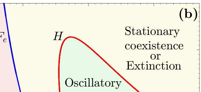
Figure 3: Results of a Monte Carlo simulation for the RMA model (1), where time-varying
r(t) is generated using p = 0.2 and “Climate variability” interval [r2 , r1 ] = [1.6, 2.7] containing
rh . Shown are 103 numerical tipping experiments (B-tipping and P-tipping) for a fixed initial
condition (N0 , P0 ) = (3, 0.002). The other parameter values are given in Appendix B, Table 1.
(a-b) The time profiles of r(t), N (t) and P (t) in a single tipping experiment. (c) The values
of r(t) (red) pre and (blue) post each tipping event. (d) States in the (N, P ) phase plane from
which the system tips to extinction via (gray dots) B-tipping and (black dots) P-tipping. (e)
The invariant measure µ(ϕλ ) of the limit cycle Γ(r) parameterised by the cycle phase ϕλ . (f)
Probability distribution of tipping phases ϕλ for (gray) B-tipping and (black) P-tipping.

(P1) Tipping from the predator-prey cycle Γ(r) to extiction occurs when r(t) decreases and does
     not cross any dangerous bifurcations of Γ(r), which is in contrast to (B1) and (B3). This
     is evidenced in Fig. 3(c) by the blue dots below r = rh depicting transitions to extinction
     when r(t) changes from rpre < rh to rpost < rpre .
(P2) Tipping occurs only from certain phases of the predator-prey cycle Γ(r), which is in contrast
     to (B2). This is evidenced by the black dots in Fig. 3(d), and the ensuing black tipping-
     phase histogram in Fig. 3(f).
(P3) The tipping phases do not correlate at all with the invariant measure µ(ϕγ ) of Γ(r) shown
     in Fig. 3(e). This is evidenced by a comparison with the black histogram in Fig. 3(f).
Since the unexpected tipping transitions occur only from certain phases of the cycle, we refer to

                                                 7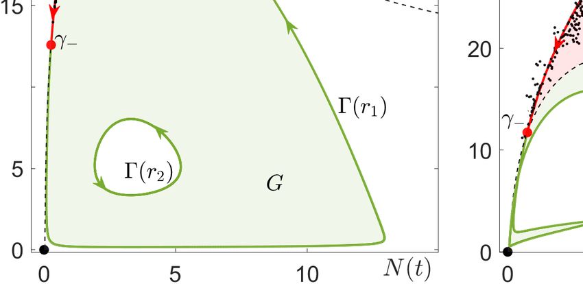
Figure 4: (a-b) and (d) The same as in Fig. 3 except for r(t) taking values from a different
“Climate variability” interval [r2 , r1 ] = [1.6, 2.5] that does not contain rh . As a result, each of
the 1000 tipping events is P-tipping. (c) The probability distribution of tipping at time t. The
other parameter values are given in Appendix B, Table 1.

this phenomenon as phase-sensitive tipping or P-tipping.
    Although P-tipping is less understood than B-tipping, it is ubiquitous and possibly even
more relevant for predator-prey interactions. In Fig. 4 we restrict climate variability in the RMA
model (1) to a closed interval [r2 , r1 ] that does not contain rh . In other words, we set r1 < rh .
Since the time-varying input r(t) cannot cross the dangerous heteroclinic bifurcation, all tipping
transitions are P-tipping events. Furthermore, owing to the absence of dangerous bifurcations of
Γ(r) in the May model (3) in Fig. 1(b), P-tipping from Γ(r) to extinction e0 is the only tipping
mechanism in Fig. 5. Note that P-tipping is more likely to occur in the May model, as shown by
shorter tipping times; compare Figs. 4(c) and 5(c).
    The numerical experiments in Figs. 4 and 5 serve as motivating examples for the development
of a general mathematical framework for P-tipping in Section 4.

4    A geometric framework for P-tipping: Partial basin in-
     stability
Motivated by the numerical experiments in Figs. 4 and 5, and the fact that P-tipping is not
captured by the classical bifurcation theory, the aim of this section is to provide mathematical
tools for analysis of P-tipping. Specifically, we develop a simple geometric framework that uses
global properties of the autonomous frozen system to study P-tipping from limit cycles in the
nonautonomous system. The key concept is basin instability. This concept was first introduced
in [14, Section 5.2] and [10] to study irreversible R-tipping from base states that are stationary
(attracting equilibria) for fixed-in-time external conditions. Here, we extend this concept to base
states that are attracting limit cycles for fixed-in-time external conditions. Our framework will
allow us to give easily testable criteria for the occurrence of P-tipping from limit cycles in general,
and explain the counter-intuitive collapses to extinction in the predator-prey systems from Sec. 3.

                                                  8
Figure 5: (a-d) The same as in Fig. 4 but for the May frozen model (3) with r(t) taking values
from the “Climate variability” interval [r2 , r1 ] = [2, 3.3]. Each of the 1000 tipping events is an
instance of P-tipping. The other parameter values are given in Appendix B, Table 1.
To define basin instability for limit cycles in general terms, we introduce p to denote the
vector of all input parameter(s), and consider the corresponding autonomous frozen system with
different but fixed-in-time values of p.
4.1 Ingredients for defining basin instability
One key ingredient of a basin instability definition is the base attractor in the autonomous frozen
system, denoted Γ(p), whose shape and position in the phase space vary with the input pa-
rameter(s) p. The second key ingredient is the basin of attraction of the base attractor, denoted
B(Γ, p), whose shape and extent may also vary with the input parameter(s) p. For non-stationary
attractors Γ(p), we work with the distance function between a solution x(t, x0 ; p) started from
an initial condition x0 and the set Γ(p):
d [x(t, x0 ; p), Γ(p)] = inf kx(t, x0 ; p) − γk,
γ∈Γ(p)
and define B(Γ, p) as the open set of all x0 whose trajectories converge to Γ(p) forward in time:
B(Γ, p) = {x0 : d [x(t, x0 ; p), Γ(p)] → 0 as t → +∞} .
We often refer to the closure of the basin of attraction of Γ(p), denoted B(Γ, p), which comprises
B(Γ, p) and its boundary, and to the basin boundary of Γ(p), which is given by the set difference
B(Γ, p)\B(Γ, p). Additionally, we assume that either all or part of the basin boundary of Γ(p) is a
basin boundary of at least two attractors. This property, in turn, requires that the autonomous
frozen system is at least bistable, meaning that it has at least one more attractor, other that
Γ(p), for the same values of the input parameter(s) p. The third key ingredient is a continuous
parameter path ∆p in the space of the input parameter(s) p. It is important that ∆p does not
cross any classical autonomous bifurcations of the base attractor Γ(p).
94.2 Definitions of basin instability for limit cycles
In short, basin instability of the base attractor on a parameter path describes the position of the
base attractor at some point on the path relative to the position of its basin of attraction at other
points on the path. Here, we define this concept rigorously for attracting limit cycles setwise.
Definition 4.1. In the autonomous frozen system, consider a continuous parameter path ∆p
with a family of hyperbolic attracting limit cycles Γ(p) that vary C 1 -smoothly with p ∈ ∆p . We
say Γ(p) is basin unstable on a path ∆p if there are two points on the path, p1 , p2 ∈ ∆p , such
that the limit cycle Γ(p1 ) is not contained in the basin of attraction of Γ(p2 ):
There exist p1 , p2 ∈ ∆p such that Γ(p1 ) 6⊂ B(Γ, p2 ). (8)
Furthermore, we distinguish two observable (or typical) cases of basin instability:
(i) We say Γ(p) is partially basin unstable on a path ∆p if, there are two points on the path,
p1 , p2 ∈ ∆p , such that the limit cycle Γ(p1 ) is not contained in the closure of the basin
of attraction of Γ(p2 ), and, for every two points on the path, p3 , p4 ∈ ∆p , Γ(p3 ) has a
non-empty intersection with the basin of attraction of Γ(p4 ):
There exist p1 , p2 ∈ ∆p such that Γ(p1 ) 6⊂ B(Γ, p2 ), and
\
Γ(p3 ) B(Γ, p4 ) 6= ∅ for every p3 , p4 ∈ ∆p . (9)
(ii) We say Γ(p) is totally basin unstable on a path ∆p if there are (at least) two points on
the path, p1 , p2 ∈ ∆p , such that Γ(p1 ) lies outside the closure of the basin of attraction of
Γ(p2 ):
\
There exist p1 , p2 ∈ ∆p such that Γ(p1 ) B(Γ, p2 ) = ∅. (10)
Remark 4.1. Additionally, there are two indiscernible (or special) cases of basin instability
for limit cycles. They cannot be easily distinguished by observation from total basin instability,
or from lack of basin instability. However, the indiscernible cases are necessary (although not
sufficient) for the onset of partial basin instability and for transitions between partial and total
basin instability.
(iii) We say Γ(p) is marginally basin unstable on a path ∆p if, in addition to (8), for every two
points on the path, p3 , p4 ∈ ∆p , the limit cycle Γ(p3 ) is contained in B(Γ, p4 ):
Γ(p3 ) ⊂ B(Γ, p4 ) for every p3 , p4 ∈ ∆p . (11)
The special case of marginal basin instability separates the typical cases of “no basin in-
stability” and “partial basin instability”. Furthermore, it is related to “invisible R-tipping”
and to transitions between “tracking” and “partial R-tipping” identified in [27].
(iv) We say Γ(p) is almost totally basin unstable on a path ∆p if there are (at least) two points
on the path, p1 , p2 ∈ ∆p , such that Γ(p1 ) does not intersect B(Γ, p2 ), and, for every two
points on the path, p3 , p4 ∈ ∆p , the limit cycle Γ(p3 ) intersects B(Γ, p4 ):
\
There exist p1 , p2 ∈ ∆p such that Γ(p1 ) B(Γ, p2 ) = ∅, and
\
Γ(p3 ) B(Γ, p4 ) 6= ∅ for every p3 , p4 ∈ ∆p . (12)
The special case of almost total basin instability separates the typical cases of “partial basin
instability” and “total basin instability”. Furthermore, it is related to transitions between
“partial R-tipping” and ”total R-tipping” described in [27].
Note that, for equilibrium base states, “partial basin instability” is not defined, whereas “marginal
basin instability” and “almost total basin instability” become the same condition.
10Guided by the approach proposed in [14], we would like to augment the classical autonomous
bifurcation diagrams for the autonomous frozen system with information about (partial) basin
instability of the base attractor Γ(p). The aim is to reveal nonautonomous bifurcations that
are not captured by classical autonomous bifurcation analysis. To illustrate basin instability of
Γ(p) in the bifurcation diagram of the autonomous frozen system, we define the region of basin
instability of Γ(p) in the space of the input parameters as follows:
Definition 4.2. In the autonomous frozen system, consider Γ(p1 ) and Γ(p2 ) from a C 1 -smooth
family of hyperbolic attracting limit cycles Γ(p). We define a region of basin instability of Γ(p1 )
as a set of all points p2 in the space of the input parameters p, such that Γ(p1 ) is not contained
in the basin of attraction of Γ(p2 ):
BI(Γ, p1 ) := {p2 : Γ(p1 ) 6⊂ B(Γ, p2 )} . (13)
To conclude this section, we show that partial basin instability of an attracting limit cycle for
the frozen system gives easily testable criteria for irreversible P-tipping in the nonautonomous
system. Specifically, partial basin instability, together with a suitable parameter change p(t), are
sufficient for irreversible P-tipping to occur.
Proposition 4.1. In the autonomous frozen system, consider a continuous parameter path ∆p ,
and a family of hyperbolic attracting limit cycles Γ(p) that vary C 1 -smoothly with p ∈ ∆p . Suppose
Γ(p) is partially basin unstable on ∆p . Then, for all p1 and p2 ∈ ∆p , an instantaneous change
from p1 to p2 gives irreversible P-tipping from Γ(p1 ) if and only if Γ(p1 ) 6⊂ B(Γ, p2 ).
Proof. An instantaneous parameter change from p1 to p2 at time t = t0 reduces the problem
to an autonomous initial value problem with initial condition x0 = x(t0 ) and fixed p = p2 . It
follows from the definition of basin of attraction that only solutions x(t, x0 ; p2 ) started from
x0 ∈ B(Γ, p2 ) are attracted to the limit cycle Γ(p2 ). Thus, if Γ(p) is partially basin unstable on
∆p and Γ(p1 ) 6⊂ B(Γ, p2 ), then there will be γ ∈ Γ(p1 ) \ B(Γ, p2 ), that give irreversible tipping,
and γ ∈ Γ(p1 ) ∩ B(Γ, p2 ), that give no tipping. Conversely, if there is irreversible P-tipping from
Γ(p1 ), then there must be γ ∈ Γ(p1 ) \ B(Γ, p2 ), which implies Γ(p1 ) 6⊂ B(Γ, p2 ).
Remark 4.2. We point out that
(i) In addition to P-tipping from the limit cycle Γ(p1 ), there can be P-tipping from any state
x0 ∈
/ B(Γ, p2 ). Examples of such P-tipping can be seen in Fig. 9(b).
(ii) Proposition 4.1 can be extended to reversible P-tipping. By “reversible” we mean that the
system leaves the stable base state only temporarily and returns to it in the long-term; e.g.
excitability [7]. Reversible P-tipping requires more general concepts of “tipping thresholds”
that are basin boundaries of a single attractor, or do not even form a basin boundary, and
“threshold instability”. We refer to [10] and [11] for more details.
(iii) Proposition 4.1 can be extended to a smoothly varying p(t), although this requires techniques
beyond the scope of this paper [27, 31]. For a smoothly varying p(t), the main differences
are that P-tipping from Γ(p) is expected to occur above some critical rate of change of p(t),
and P-tipping may occur from phases that are not basin unstable.
5 Partial basin instability and P-tipping in predator-prey
models
In this section, we start with classical autonomous bifurcation analysis of the predator-prey
frozen systems (1) and (3) to identify parameter regions with bistability between predator-prey
cycles and extinction. Then, we show that predator-prey cycles can be partially basin unstable
on parameter paths ∆r that lie within these regions of bistability. Finally, we demonstrate
that partial basin instability of predator-prey cycles on a path ∆r explains the counter-intuitive
and phase-sensitive collapses from oscillatory coexistence to extinction, and gives simple testable
criteria for the occurrence of P-tipping in the nonautonomous predator-prey system.
11Figure 6: Two-parameter bifurcation diagrams for (a) the autonomous RMA frozen model (1) in
the (r, δ) parameter plane, and (b) the autonomous May frozen model (3) in the (r, q) parameter
plane. The other parameter values are given in Appendix B, Table 1.
5.1 Classical bifurcation analysis: Limit cycles and bistability
There are four ecologically relevant parameter regions in the predator-prey frozen systems (1)
and (3), shown in Figure 6. These regions have qualitatively different dynamics that can be
summarised in terms of stable states as follows:
• Oscillatory Coexistence or Extinction: The system is bistable and can either settle at the
extinction equilibrium e0 , or self-oscillate as it approaches the predator-prey limit cycle
Γ(r). Here is where P-tipping may occur; see the green regions in Fig. 6.
• Stationary Coexistence or Extinction: The system is bistable and can settle either at the
extinction equilibrium e0 , or at the coexistence equilibrium e3 (r); see the yellow regions in
Fig. 6.
• Prey Only or Extinction: The system is bistable and can settle either at the extinction
equilibrium e0 , or at the prey-only equilibrium e1 (r); see the pink region in Fig. 6(a).
• Extinction: The system is monostable and can only settle at the extinction equilibrium e0 ;
see the pink regions in Fig. 6.
The region boundaries are obtained via two-parameter bifurcation analysis using the numerical
continuation software XPPAUT [74]. This extends our discussion of the one-parameter bifurca-
tion diagrams from Fig. 1. We refer to [75] for more details on bifurcation theory.
We start with the autonomous RMA frozen model (1), consider the climatic parameter r to-
gether with the predator mortality rate δ, and examine the bifurcation structure in the (r, δ)
parameter space in Fig. 6(a). The dynamics are organised by the codimension-two double-
transcritical bifurcation point T T , due to an intersection of two transcritical bifurcation curves,
namely T1 , along which e1 (r) and e2 (r) meet and exchange stability, and T2 , along which e1 (r)
and e3 (r) meet and exchange stability2 . T T is the origin of the Hopf H and heteroclinic h bi-
furcation curves, both of which are subcritical (dashed) near T T . Furthermore, H changes from
subcritical (dashed) to supercritical (solid) at the codimension-two generalised Hopf bifurcation
point GH, from which the curve Fl of the fold of limit cycles emerges. The stable limit cycle
Γ(r) shrinks onto e3 (r) along the supercritical (solid) part of H, or collides with an unstable
2 Since a Hopf bifurcation for a complex variable z = r eiθ is a transcritical bifurcation for the “amplitude”
variable ρ = r2 , we expected the unfolding of T T to be the same as one of the unfoldings in the “amplitude
equations” for the Hopf-Hopf bifurcation. This, however, is not the case. The unfolding of T T is akin, although
not identical, to the unfolding of the “amplitude equations” for the Hopf-Hopf bifurcation point in subregion 6 of
the “dificult” case from Ref. [75, Sec.8.6].
12limit cycle and disappears along Fl . Then, Fl has another endpoint on h. This point is the
codimension-two resonant heteroclinic bifurcation point Rh, where h changes from subcritical
(dashed) to supercritical (solid). The stable limit cycle Γ(r) collides simultaneously with two
saddles, e1 (r) and e2 , and disappears along the supercritical (solid) part of h. Our main focus
is on the (green) region of bistability between oscillatory coexistence Γ(r) and extinction e0 .
This region is bounded by the three bifurcation curves along which the stable limit cycle Γ(r)
disappears: the fold of limit cycles Fl , the (solid) supercritical part of the Hopf curve H, and the
(solid) supercritical part of the homoclinic curve h. Finally, note that there is a third transcrit-
ical bifurcation curve corresponding to T0 in the inset of Fig. 1(a). This curve is not shown in
Fig 6(a) for clarity reasons; it lies very close to T1 and is not relevant to our study.
For the autonomous May frozen model (3), we consider the climatic parameter r together with
q. Here, q specifies the minimum prey-to-predator biomass ratio to allow predator population
growth, and can be thought of as an ‘equivalent’ of the predator mortality rate from the RMA
frozen model (1). The qualitative picture, shown in Fig. 6(b), is very similar to that for the RMA
frozen model in Fig. 6(a). The main difference is that the organising centre for the dynamics is
the codimension-two Bogdanov-Takens bifurcation point BT . Furthermore, instead of the three
transcritical bifurcation curves there is just one, denoted T , along which e1 (r) and e2 meet and
become degenerate, together with a single (dark blue) curve Fe of fold of equilibria, where e3 (r)
and e4 (r) become degenerate and disappear.
As a result, the region of “Extinction or Prey Only” is gone, leaving just three ecologically
relevant parameter regions. The heteroclinic bifurcation curve h is replaced by a homoclinic
bifurcation curve h∗ , along which Γ(r) collides with one saddle, namely e4 (r), and disappears.
The resonant heteroclinic point Rh is replaced by a resonant homoclinic point Rh∗ . Most inter-
estingly, except for the change from h to h∗ , the boundary of the (green) region of bistability
between oscillatory coexistence Γ(r) and extinction e0 consists of the same bifurcation curves as
in the RMA frozen model.
5.2 Partial basin instability of predator-prey cycles
We now concentrate on the bistable regions labelled “Oscillatory Coexistence or Extinction”,
apply Definitions 4.1 and 4.2 to predator-prey cycles, and show that
• Predator-prey cycles Γ(r) can be partially basin unstable on suitably chosen parameter
paths.
• Both predator-prey models have large parameter regions of partial basin instability. When
superimposed onto classical bifurcation diagrams, these regions reveal P-tipping instabilities
that cannot be captured by the classical autonomous bifurcation analysis.
• Partial basin instability of Γ(r) in the frozen system is sufficient for the occurrence of
P-tipping in the nonautonomous system.
The base attractor is the predator-prey limit cycle Γ(r), and the second attractor is the
extinction equilibrium e0 . The basin boundary of Γ(r) and e0 is the stable invariant manifold of
the saddle equilibrium es (r):
θ(r) := W s (es (r)) = (N0 , P0 ) ∈ R2 : (N (t), P (t)) → es (r) as t → +∞ .
In the RMA frozen model, es (r) is the saddle Allee equilibrium e2 , whereas in the May frozen
model, es (r) is the saddle coexistence equilibrium e4 (r) that lies near the repelling Allee equi-
librium e2 . To uncover the full extent of partial basin instability for the predator-prey cycles
Γ(r), we fix a point p1 that lies within the region labelled “Oscillatory Coexistence or Extinc-
tion”; see Figs. 7(a) and 8(a). Then, we apply definition (13) to identify all points p2 within this
region such that the predator-prey limit cycle Γ(p1 ) is not contained in the closure of the basin
of attraction of Γ(p2 ). The ensuing (light grey) regions of partial basin instability bounded by
the (dark grey) curves of marginal basin instability are superimposed on the classical bifurcation
diagrams in Figs. 7(a) and 8(a). Note that the basin instability regions BI(Γ, p1 ) depend on the
choice of p1 , and are labelled simply BI for brevity. To illustrate the underlying mechanism in
the (N, P ) phase plane, we to restrict to parameter paths ∆r that are straight horizontal lines
13Figure 7: (a) The two-parameter bifurcation diagram for the autonomous RM frozen model (1)
from Fig. 6(a) with the addition of the (grey) region of partial basin instability, BI(Γ, p1 ) for
p1 = (2.47, 2.2), as defined by (13), and the parameter path ∆r from p1 . (b) The range of
basin unstable phases for the predator-prey limit cycle Γ(r) along ∆r . (c)–(e) Selected (N, P )
phase portraits showing (c) no basin instability for r2 = 2.05, (d) marginal basin instability for
r2 = 1.923, and (e) partial basin instability of Γ(r) on ∆r for r2 = 1.8. Basin stable parts of Γ(r)
are shown in green, basin unstable parts of Γ(r) are shown in red. The other parameter values
are given in Appendix B, Table 1.
from p1 in the direction of decreasing r. In other words, we set p = r; see Figs. 7(a) and 8(a).
When r2 ∈ ∆r lies on the dark grey curve of marginal basin instability, there is a single point
of tangency between Γ(r1 ) and and θ(r2 ), denoted γ± in Figs. 7(d) and 8(d). When r2 ∈ ∆r
lies within the light grey region of partial basin instability, there are two points of intersection
between Γ(r1 ) and and θ(r2 ), denoted γ− and γ+ in Figs. 7(e) and 8(e). These two points bound
the (red) part of the cycle that is basin unstable. The corresponding basin unstable phases are
shown in Figs. 7(b) and 8(b). Suppose that r(t) = r1 , and a trajectory of the nonautonomous
system is on the same side of θ(r2 ) as the (red) basin unstable part of Γ(r1 ). Then, when r(t)
changes from r1 to r2 , the trajectory finds itself in the basin of attraction of the extinction
equilibrium e0 , and will thus approach e0 .
The striking similarity is that predator-prey cycles from both models exhibit partial basin
instability upon decreasing r. This corresponds to climate-induced decline in the resources or
in the quality of habitat. Furthermore, while the predator-prey cycle in the May model has
a noticeably wider range of basin unstable phases, neither cycle appears to be totally basin
unstable. All these observations are consistent with the counter-intuitive properties (P1)–(P3)
of P-tipping identified in the numerical experiments in Sec. 3.
5.3 Partial basin instability explains P-tipping
Now, we can demonstrate that partial basin instability of Γ(r) in the autonomous predator-prey
frozen systems explains and gives simple testable criteria for the occurrence of P-tipping in the
14Figure 8: (a) The two-parameter bifurcation diagram for the autonomous May frozen model (3)
from Fig. 6(b) with the addition of the (grey) region of partial basin instability, BI(Γ, p1 ) for
p1 = (3.3, 205), as defined by (13), and the parameter path ∆r from p1 . (b) The range of
basin unstable phases for the predator-prey limit cycle Γ(r) along ∆r . (c)–(e) Selected (N, P )
phase portraits showing (c) no basin instability for r2 = 2.82, (d) marginal basin instability for
r2 = 2.41, and (e) partial basin instability of Γ(r) on ∆r for r2 = 2. Basin stable parts of Γ(r)
are shown in green, basin unstable parts of Γ(r) are shown in red. The other parameter values
are given in Appendix B, Table 1.
nonautonomous systems. The families of attracting predator-prey limit cycles Γ(r), and their
basin boundaries θ(r), are the two crucial components of the discussion below.
First, recall the numerical P-tipping experiments from Sec. 3, and focus on the crescent shaped
‘clouds’ of states from which P-tipping occurs; see the black dots Figs. 4 and 5. Second, recognise
that each P-tipping event occurs for a different value of rpre ∈ [r2 , r1 ], and thus from a different
predator-prey cycle Γ(rpre ). Therefore, we must consider the union of all cycles from the family
along the parameter path ∆r bounded by r2 and r1 :
[
G := Γ(r), (14)
r∈[r2 ,r1 ]
which is shown in Fig. 9. Furthermore, we use the basin boundary θ(r2 ) of the cycle Γ(r2 ) at
the end of the path to divide G into its (light green) basin stable part and (pink) basin unstable
part on ∆r with r ∈ [r2 , r1 ]. The ‘clouds’ of states from which P-tipping occurs agree perfectly
with the basin unstable part of G. A few black dots that lie slightly outside the basin unstable
part of G in Fig. 9(b) correspond to those P-tipping events that occur from states that are not
on the limit cycle Γ(rpre ), as pointed out in Prop. 4.1 and Rmk. 4.2(i). Those P-tipping events
occur when the interval ` during which r(t) = rpre is too short for the trajectory to approach
Γ(rpre ).
In other words, Fig. 9 is an illustration of Prop. 4.1. The figure applies the general concept
of partial basin instability on a parameter path from Def. 4.1 to predator-prey cycles Γ(r) of the
autonomous RMA (1) and May (3) frozen systems. The numerical results show that partial basin
15Figure 9: The concept of partial basin instability on a parameter path ∆r with r ∈ [r2 , r1 ]
(see Def. 4.1) is applied to the union G of all predator-prey limit cycles Γ(r) on the path (see
Eq.(14)) to explain the counter-intuitive P-tipping phenomenon uncovered Figs. 4 and 5. The
(black dots) states from which the system P-tips to extinction agree perfectly with the (pink)
basin unstable parts of G for (a) the RMA model (1) with r1 = 2.5, r2 = 1.6, and δ = 2.2, and
(b) the May model (3) with r1 = 3.3, r2 = 2, and q = 205. The other parameter values are given
in Appendix B, Table 1.
instability on a path ∆r in the predator-pray frozen systems with a fixed-in-time r is necessary for
the occurrence of irreversible P-tipping in the nonautonomous systems with piecewise constant
r(t).
6 Conclusions
This paper studies nonlinear tipping phenomena, or critical transitions, in nonautonomous dy-
namical systems with time-varying external inputs. In addition to the well-known critical factors
for tipping in systems that are stationary in the absence of external inputs (bifurcation, rate of
change, and noise) [3], we identify here phase of a cycle as a new critical factor in systems that
are cyclic in the absence of external inputs.
To illustrate the new tipping phenomenon in a realistic setting, we consider two paradigmatic
predator-prey models with an Allee effect, namely the Rosenzweig-MacArthur model [38] and the
May model [39]. We describe temporal changes in the carrying capacity of the ecosystem with
real climate variability records from different communities in the boreal and deciduous-boreal
forest [45], and use realistic parameter values for the Canada lynx and snowshoe hare system [43,
44]. Monte Carlo simulation reveals a robust phenomenon, where a drop in the carrying capacity
tips the ecosystem from a predator-prey limit cycle to extinction. The special and somewhat
counter-intuitive result is that tipping occurs: (i) without crossing any bifurcations, and (ii) only
from certain phases of the cycle. Thus, we refer to this phenomenon as phase-sensitive tipping
or simply P-tipping.
Motivated by the outcome of the simulation, we develop an accessible and general mathemati-
cal framework to analyse P-tipping and reveal the underlying dynamical mechanism. Specifically,
we employ notions from set-valued dynamics to extend the geometric concept of basin instability,
introduced by O’Keeffe and Wieczorek [14] for equilibria, to limit cycles. The main idea is to
consider the autonomous frozen system with different but fixed-in-time values of the external
input along some parameter path, and examine the position of the limit cycle at some point on
the path relative to the position of its basin of attraction at other points on the path. First, we
define different types of basin instability for limit cycles, and focus on partial basin instability that
does not exist for equilibria. Second, we show that partial basin instability in the autonomous
frozen system is sufficient for the occurrence of P-tipping in the nonautonomous system with a
16suitable external input. Third, we relate our results to the results of Alkhayuon and Ashwin [27]
on rate-induced tipping from limit cycles.
We then apply the general framework to the ecosystem models and explain the counter-
intuitive and phase-sensitive transitions from predator-prey limit cycles to extinction. We use
classical autonomous bifurcation analysis to identify parameter regions with bistability between
predator-prey cycles and extinction. In this way, we show that predator-prey cycles can be
partially basin unstable on typical parameter paths within these bistability regions. Moreover,
we superimpose regions of partial basin instability onto classical autonomous bifurcation diagrams
to reveal P-tipping instabilities that are robust but cannot be captured by the classical bifurcation
analysis.
We believe that this approach will enable scientists to uncover P-tipping in many different
cyclic systems from applications, ranging from natural science and engineering to economics. For
example, the predator-prey paradigm is found across biological applications modelling, including
epidemiology [76], pest control [77], fisheries [78], cancer [79, 80], and agriculture [81, 82]. The
fundamental relationship described in predator-prey models also appears in many areas outside
of the biological sciences, with recent examples including atmospheric sciences [83], economic
development [64, 65], trade and financial crises [84, 85, 86], and land management [87]. Exter-
nal disturbances of different kinds exist in all of these systems, suggesting that the P-tipping
behaviours discovered in this paper are of broad practical relevance.
Furthermore, the concept of P-tipping from base states that are attracting limit cycles with
regular basin boundaries naturally extends to more complicated base states, such as quasiperiodic
tori and chaotic attractors, and to irregular (e.g. fractal) basin boundaries [29, 88, 31, 32].
Defining phase for more complicated cycles in higher dimensions and non-periodic base states
will usually require a different approach. For example, one can work with a time series of a
single observable and use the Hilbert transform to construct the complex-valued analytic signal,
and then extract the so-called instantaneous phase [89, 90]. This phase variable may provide
valuable physical insights into the problem of P-tipping when the polar coordinate approach
does not work, or when the base attractor or its basin boundary have complicated geometry and
are difficult to visualise. Such systems will exhibit even more counter-intuitive behaviour, but
their analysis requires different and more advanced mathematical techniques.
Another interesting research question is that of early warning indicators for P-tipping. In the
past decade, many studies of noisy real-world time-series records revealed prompt changes in the
statistical properties of the data prior to tipping [1, 22, 91, 23], which appear to be generic for
tipping from equilibria. However, it is unclear if these statistical early warning indicators appear
for P-tipping, or if one needs to identify alternatives such as Finite Time Lyapunov Exponent
(FTLE) [92].
Data Accessibility and Authors’ Contributions
The codes used to conduct simulations and generate figures are available via the GitHub repos-
itory [93]. All authors contributed to the numerical computations and to the writing of the
manuscript. HA and SW contributed to the theoretical results in Sec. 4
Funding and Acknowledgements
HA and SW are funded by Enterprise Ireland grant No. 20190771. RCT is funded by NSERC
Discovery Grant RGPIN-2016-05277. The authors would like to thank Johan Dubbeldam, Cris
Hasan, Bernd Krauskopf, Jessa Marley, and Emma McIvor for their insightful comments on this
work.
References
[1] Marten Scheffer, Jordi Bascompte, William A Brock, Victor Brovkin, Stephen R Carpenter,
Vasilis Dakos, Hermann Held, Egbert H Van Nes, Max Rietkerk, and George Sugihara.
Early-warning signals for critical transitions. Nature, 461(7260):53–59, 2009.
17[2] Timothy M Lenton, Hermann Held, Elmar Kriegler, Jim W Hall, Wolfgang Lucht, Stefan
Rahmstorf, and Hans Joachim Schellnhuber. Tipping elements in the earth’s climate system.
Proceedings of the national Academy of Sciences, 105(6):1786–1793, 2008.
[3] Peter Ashwin, Sebastian Wieczorek, Renato Vitolo, and Peter Cox. Tipping points in open
systems: bifurcation, noise-induced and rate-dependent examples in the climate system.
Philosophical Transactions of the Royal Society A: Mathematical, Physical and Engineering
Sciences, 370(1962):1166–1184, 2012.
[4] J Michael T Thompson, HB Stewart, and Y Ueda. Safe, explosive, and dangerous bifurca-
tions in dissipative dynamical systems. Physical Review E, 49(2):1019, 1994.
[5] J Michael T Thompson and Jan Sieber. Climate tipping as a noisy bifurcation: a predictive
technique. IMA Journal of Applied Mathematics, 76(1):27–46, 2011.
[6] Christian Kuehn. A mathematical framework for critical transitions: Bifurcations, fast–slow
systems and stochastic dynamics. Physica D: Nonlinear Phenomena, 240(12):1020–1035,
2011.
[7] Sebastian Wieczorek, Peter Ashwin, Catherine M Luke, and Peter M Cox. Excitability
in ramped systems: the compost-bomb instability. Proceedings of the Royal Society A:
Mathematical, Physical and Engineering Sciences, 467(2129):1243–1269, 2011.
[8] Clare Perryman and Sebastian Wieczorek. Adapting to a changing environment: non-
obvious thresholds in multi-scale systems. Proceedings of the Royal Society A: Mathematical,
Physical and Engineering Sciences, 470(2170):20140226, 2014.
[9] Anna Vanselow, Sebastian Wieczorek, and Ulrike Feudel. When very slow is too fast-collapse
of a predator-prey system. Journal of theoretical biology, 479:64–72, 2019.
[10] Sebastian Wieczorek, Peter Ashwin, and Chun Xie. Rate-induced tipping: Regular thresh-
olds, edge states and testable criteria. in preparation, 2021.
[11] Sebastian Wieczorek, Peter Ashwin, and Chun Xie. Rate-induced tipping: Quasithresholds,
canards and testable criteria. in preparation, 2021.
[12] Christian Kuehn and Iacopo P Longo. Estimating rate-induced tipping via asymptotic series
and a melnikov-like method. arXiv preprint arXiv:2011.04031, 2020.
[13] Marten Scheffer, Egbert H Van Nes, Milena Holmgren, and Terry Hughes. Pulse-driven loss
of top-down control: the critical-rate hypothesis. Ecosystems, 11(2):226–237, 2008.
[14] Paul E O’Keeffe and Sebastian Wieczorek. Tipping phenomena and points of no return in
ecosystems: Beyond classical bifurcations. SIAM Journal on Applied Dynamical Systems,
19(4):2371–2402, 2020.
[15] Peter Ashwin, Clare Perryman, and Sebastian Wieczorek. Parameter shifts for nonau-
tonomous systems in low dimension: bifurcation-and rate-induced tipping. Nonlinearity,
30(6):2185, 2017.
[16] Hassan Alkhayuon, Peter Ashwin, Laura C Jackson, Courtney Quinn, and Richard A Wood.
Basin bifurcations, oscillatory instability and rate-induced thresholds for atlantic meridional
overturning circulation in a global oceanic box model. Proceedings of the Royal Society A,
475(2225):20190051, 2019.
[17] Michael Hartl. Non-autonomous random dynamical systems: Stochastic approximation and
rate-induced tipping. PhD thesis, Imperial College London, 2019.
[18] Claire Kiers and Christopher KRT Jones. On conditions for rate-induced tipping in multi-
dimensional dynamical systems. Journal of Dynamics and Differential Equations, 32(1):483–
503, 2020.
18You can also read