Comparison of Two Ensemble Kalman-Based Methods for Estimating Aquifer Parameters from Virtual 2-D Hydraulic and Tracer Tomographic Tests - MDPI
←
→
Page content transcription
If your browser does not render page correctly, please read the page content below
geosciences
Article
Comparison of Two Ensemble Kalman-Based
Methods for Estimating Aquifer Parameters from
Virtual 2-D Hydraulic and Tracer Tomographic Tests
Emilio Sánchez-León           , Daniel Erdal † , Carsten Leven     and Olaf A. Cirpka *
 Center for Applied Geoscience, University of Tübingen, Schnarrenbergstrasse 94-96, 72076 Tübingen, Germany;
 emilio.sanchez@uni-tuebingen.de (E.S.-L.); daniel.erdal@uni-tuebingen.de (D.E.);
 carsten.leven-pfister@uni-tuebingen.de (C.L.)
 * Correspondence: olaf.cirpka@uni-tuebingen.de
 † Current address: Tyréns AB, Peter Myndes Backe 16, 118 86 Stockholm, Sweden.

 Received: 28 May 2020; Accepted: 14 July 2020; Published: 17 July 2020

 Abstract: We compare two ensemble Kalman-based methods to estimate the hydraulic conductivity
 field of an aquifer from data of hydraulic and tracer tomographic experiments: (i) the Ensemble
 Kalman Filter (EnKF) and (ii) the Kalman Ensemble Generator (KEG). We generated synthetic
 drawdown and tracer data by simulating two pumping tests, each followed by a tracer test.
 Parameter updating with the EnKF is performed using the full transient signal. For hydraulic
 data, we use the standard update scheme of the EnKF with damping, whereas for concentration
 data, we apply a restart scheme, in which solute transport is resimulated from time zero to the next
 measurement time after each parameter update. In the KEG, we iteratively assimilate all observations
 simultaneously, here inverting steady-state heads and mean tracer arrival times. The inversion
 with the dampened EnKF worked well for the transient pumping-tests, but less for the tracer tests.
 The KEG produced similar estimates of hydraulic conductivity but at significantly lower costs.
 We conclude that parameter estimation in well-defined hydraulic tests can be done very efficiently by
 iterative ensemble Kalman methods, and ambiguity between state and parameter updates can be
 completely avoided by assimilating temporal moments of concentration data rather than the time
 series themselves.

 Keywords: hydraulic tomography; tracer tomography; temporal moments; virtual experiments;
 Ensemble-Kalman Filter; Kalman Ensemble Generator

1. Introduction
      Reliable predictions of water and solute transport in groundwater depend, to a large extent,
on the resolution at which aquifer heterogeneity is resolved. In inverse models, the model
parameters (e.g., the hydraulic conductivity field) are derived from observations of model states
(e.g., hydraulic heads, soil water content, and solute concentrations). To optimize computational
costs and increase the resolution of estimated parameter distributions, many inversion methods have
been developed [1–3]. Gradient-based techniques derived from the Gauss–Newton method require
computing the sensitivity of all observations with respect to all parameters in each iteration, imposing
prohibitive computational costs if a highly discretized model is used and many observations are
available. In the pilot-point method, parameters are estimated at a limited number of points and
interpolated everywhere else within the domain by kriging [4–6], which may be interpreted either
as a variant of geostatistical inversion (see below), provided that prior knowledge is considered
consistently, or as parameterization using the covariance functions centered about the pilot points as
base functions [7].

Geosciences 2020, 10, 276; doi:10.3390/geosciences10070276                 www.mdpi.com/journal/geosciences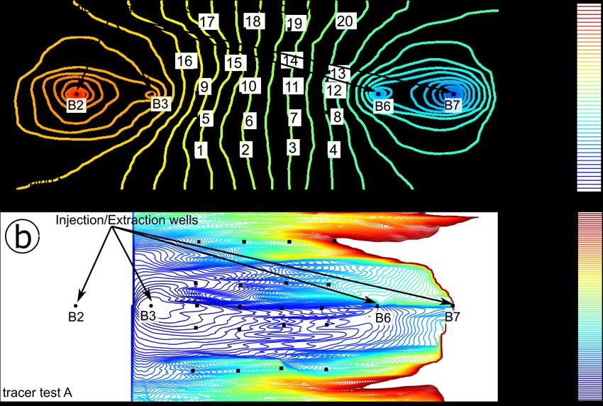
Geosciences 2020, 10, 276                                                                         2 of 27

     Geostatistical inversion techniques consider the parameters as spatially correlated random
variables. Prior knowledge is expressed by the covariance function of the parameters, which are
conditioned on dependent measurements such as hydraulic heads or tracer breakthrough curves [8–12].
The sensitivities of individual observations on the parameter fields are typically obtained by solving
as many adjoint problems as there are measurements [13], increasing the computational costs when
transient processes or data from tomographic tests are considered. To reduce the number of adjoint
problems, data may be aggregated by considering temporal moments of the time series [11,14–16].
To further ease the computational demands of large-dimensional problems, the authors of [17,18]
propose a geostatistical inversion technique (Principal Component Geostatistical Approach (PCGA))
where the complete Jacobian matrix is not explicitly calculated. Instead, the required derivatives are
computed by performing matrix-vector multiplications. The computational cost of the PCGA scales
linearly with the number of unknowns. In yet another variant of the geostatistical inversion model,
the authors of [19] present an estimator that reduces the dimensionality of the problem (Reduced-Order
Successive Linear Estimator), by approximating the covariance and cross-covariances needed in the
Successive Linear Estimator (SLE) algorithm [20] with eigenvalue decomposition of the parameter
covariance matrix. More recently, Parker et al. [21] introduced a new derivative-free approach for
parameter estimation in hydrogeology, which combines evolutionary algorithms (e.g., particle swarm)
and Ensemble Kalman filters.
     Sequential data assimilation and Kalman filter methods have increasingly been used in
groundwater applications [22–33]. Data assimilation is a procedure in which noisy observations
and simulation results at the current state of a system are merged. The model states are corrected
to minimize the difference between modeled and real observations. Model states at points where
no observations exist are updated according to the correlation with the observations, which is exact
only for linear dependencies and multi-Gaussian distributions. The model simulations are then run
forward in time until new observations are available and the errors are evaluated again, defining a
forecast/correction cycle. To improve the predictions of the corrected model, the model-state vector
may be augmented by model parameters, which are updated together with the states. Thisr is of
particular relevance in hydrogeological applications, where model predictions strongly depend on
parameter values.
     Recently, ensemble Kalman-based methods have become popular methods in hydrogeology, with the
Ensemble Kalman Filter (EnKF) being the most used approach [34–36]. Formally, the conditioning in the
linearized geostatistical approach and the ensemble Kalman-based methods is identical. However, in
the latter, the covariance matrices needed for updating are evaluated by ensemble averaging within
Monte Carlo simulations rather than by linearized uncertainty propagation. By this, costly calculations
of sensitivities are avoided. As these methods work with an ensemble of updated stochastic realizations,
they provide parameter uncertainty estimates without additional computational costs.
     To tune the capabilities of ensemble Kalman-based methods, many adaptations have been made
to the original formulations. The vector of model states may be augmented by parameter values,
which are also updated in the data assimilation [23,26]. To estimate hydraulic conductivity fields,
some studies exclusively relied on hydraulic-head observations [26,32,37], while others used also
concentration data [25,27,29]. Nowak [38] modified the standard EnKF for updating only model
parameters (the Ensemble Kalman Generator), and Schöniger et al. [39] applied it to estimate the
hydraulic conductivity distribution of a 3-D groundwater flow model using data from a virtual
hydraulic tomography test.
     Sequential data assimilation is appealing for real-time models, in which simulated model states
are updated by continuous monitoring data. Although hydraulic parameters can jointly be estimated
in real-time model applications, the joint uncertainty of material properties and boundary conditions
can lead to biased parameter estimates. Hydraulic tests, in which the groundwater response to a
well-defined disturbance is measured, are better suited for the estimation of hydraulic properties.
However, a single hydraulic test may not contain enough information to reliably infer spatial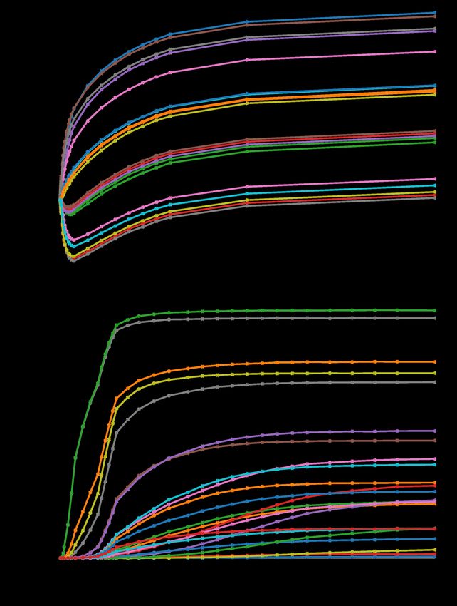
Geosciences 2020, 10, 276                                                                            3 of 27

distributions of hydraulic parameters. To overcome data scarcity, field methods with a tomographic
layout have gained the attention of the scientific community. The idea behind a hydrogeological
tomographic survey is to sequentially stimulate the aquifer at multiple locations, and measure the
corresponding response at many observation points. The observations are sequentially or jointly
inverted to estimate hydraulic parameters. The most common application of a hydrogeological
tomographic method is hydraulic tomography [18,40–64], which involves a sequence of pumping
tests performed at multiple injection or extraction wells, and measuring the hydraulic-head changes
at many locations distributed throughout the aquifer. However, the diffusive propagation of the
hydraulic-head signal limits the information contained in head data, even with a tomographic
layout [65,66]. Recent studies suggest to integrate data of different types during model inversion,
e.g., hydraulic heads and tracer concentrations [16].
      Tracer tomography has been suggested as a field method to obtain large tracer datasets.
It may be used to infer not only flow-related aquifer parameters such as hydraulic conductivity,
but also important transport parameters such as porosity and dispersivities. In analogy to hydraulic
tomography, tracer tomography involves a series of tracer tests with the tracer injection being
constrained to a specific portion of the aquifer. The tomographic layout is achieved by shifting the
injection interval for each test and monitoring the tracer plume at different locations and depths [67–70].
The importance of tracer data for aquifer characterization lies in the close relation between the
advective propagation of solutes and the underlying velocity field, which depends on the spatial
distribution of hydraulic properties. Furthermore, differences in the sensitivity patterns of different
data types improve the resolution and reduce the uncertainty of the estimated parameters [16,68,71,72].
Although advantages of incorporating tracer data from tomographic experiments in parameter
estimation have been demonstrated in several numerical [16,68,71,73,74] and laboratory [69,72] studies,
tracer tomography has been implemented in field experiments only recently [70,75].
      The work presented in this paper is motivated by the recent developments of tracer tomography
on the field scale, and the potential of ensemble Kalman-based methods for improving the estimation of
aquifer parameters. We study the performance of two ensemble Kalman approaches in the estimation
of spatially distributed aquifer parameters of synthetic groundwater-flow and solute-transport models:
the Ensemble Kalman Filter (EnKF) and the Kalman Ensemble Generator (KEG). The advantage of
using synthetic data is that true parameter fields, intended to be retrieved by the inverse method,
are known, making an objective comparison between variants of the inverse schemes possible.
The two approaches tested in this study differ in the update scheme and data type that can be
used. Although the sequential time-step updating scheme of the EnKF fits well with transient records,
the KEG uses all observations at once to update parameters, and therefore compressed transient signals
such as their temporal moments could be used. Different applications of these ensemble Kalman-based
methods for the assimilation of hydraulic and tracer test data can be found in the literature, but their
application to data from tracer-tomographic experiments has not been reported.
      We define a synthetic case study based on the experimental design of Doro et al. [70], but consider
the injection of a solute tracer instead of heat, avoiding issues related to heat diffusivity. As a case
study that resembles a real aquifer, we mimic the aquifer located at the hydrogeological research site
Lauswiesen, in which previous tomographic experiments have been performed [62,70]. The numerical
models and the test design consider both the hydrogeological characteristics of the aquifer and
the available infrastructure for the performance of hydraulic and tracer tomographic tests, but it is
restricted to two spatial dimensions to expedite the calculations. For the EnKF, a transient groundwater
flow and solute transport model was set up using HydroGeoSphere [76], whereas for the KEG, we used
a numerical model implemented in Matlab that directly solves for two-dimensional steady-state
hydraulic heads and temporal moments of tracer concentration. In ongoing research, we apply
the EnKF and KEG to real data collected during a field implementation of a hydraulic and tracer
tomography experiment, where the true parameter fields are not known and additional conceptual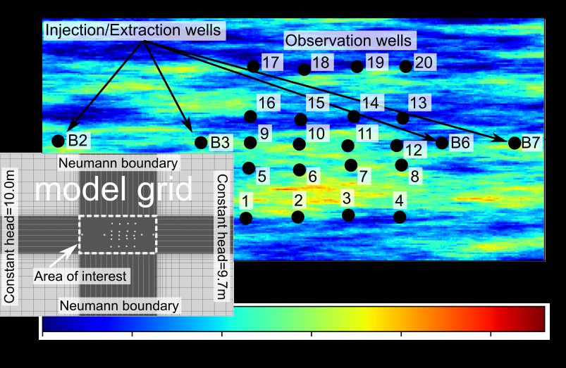
Geosciences 2020, 10, 276                                                                           4 of 27

uncertainties and measurement bias may arise. The outcome of this research will be presented in a
follow-up publication.
     This paper is organized as follows. Section 2 reviews the governing equations describing
groundwater flow and solute transport. Section 3 describes the underlying theory of parameter
estimation using ensemble Kalman-based methods. Section 4 briefly describes our numerical
implementation of a synthetic hydraulic- and tracer-tomography experiment, while Section 5 explains
the application of the EnKF and KEG to the estimation of parameters by assimilating data from those
synthetic tomography experiments. We present results and discuss them in Section 6. This work ends
with conclusions and recommendations in Section 7.

2. Governing Equations
     Transient groundwater flow in a porous aquifer can be described by the groundwater
flow equation:
                                     ∂h
                                  S0    − ∇ · (K∇h) = W0                            (1)
                                     ∂t
subject to the following initial and boundary conditions:

                                           h = h0 at t = t0 ∀x                                         (2)

                                            h = hin at Γin ∀t                                          (3)

                                            h = hout at Γout ∀t                                        (4)

                                   n̂ · (−K∇h) = q f ix (x) at Γno ∀tt                                 (5)

in which S0 [L−1 ] is the specific storativity, h [L] is the hydraulic head, t [T] denotes time, t0 [T]
refers to the initial time, K [LT−1 ] is the tensor-field of hydraulic conductivity, W0 [T−1 ] represents
volumetric sources or sinks (e.g., injection/extraction wells), Γin and Γout are Dirichlet boundaries at
the in- and outflow of the domain, respectively, and Γno represents Neumann boundaries defined along
the boundaries of the domain where the normal flux q f ix [LT−1 ] is known (e.g., q f ix = 0 at no-flow
boundaries). h0 [L] represents initial hydraulic heads, hin [L] and hout [L] are fixed hydraulic heads
along Γin and Γout , respectively, and n̂ is the unit vector normal to the boundary pointing outwards.
The specific discharge q [LT−1 ] follows Darcy’s law (q = −K∇h).
     Assuming an idealized tracer (i.e., non-sorbing, non-reacting, and not changing fluid or matrix
properties) introduced via the section Γin,c of the inflow boundary, its transport in groundwater is
commonly described by the advection–dispersion equation:

                                          ∂c
                                      n      + ∇ · (v − nD∇c) = 0                                      (6)
                                          ∂t
subject to the following initial and boundary conditions:

                                            c = 0 at t = 0 ∀x                                          (7)

                                       c(t, x) = cin (t, x) at Γin,c                                   (8)

                                      n̂ · (D∇c) = 0 at Γ\Γin,c ∀t                                     (9)

in which c [ML−3 ] is the solute concentration, n [L3 L−3 ] is the porosity, D [L2 T−1 ] is the dispersion
tensor, Γ represents all domain boundaries, and cin [ML−3 ] is a known time- and location-dependent
concentration along the inflow boundary Γin,c . The seepage velocity v [LT−1 ] is defined as

                                                       q
                                                  v=                                                  (10)
                                                       n
Geosciences 2020, 10, 276 5 of 27
and the dispersion tensor D [L2 T−1 ] is commonly parameterized as [77]
vi v j
Di,j = (α − αt ) + δij ( De + αt ||v||) (11)
||v|| l
in which vi [LT−1 ] is the i-th component of the velocity vector, αl [L] and αt [L] are the longitudinal and
transverse dispersivities, respectively, De [L2 T−1 ] is the pore diffusion coefficient, ||v|| is the absolute
value of seepage velocity, and δij is the Kronecker delta which is unity for i = j, and zero otherwise.
In many aquifers, anomalous transport characterized by early breakthrough and long tailing has
been observed [78,79]. To account for unresolved small-scale variability in hydraulic parameters and
simulate breakthrough curves affected by tailing, it is a common approach to further parameterize the
transport processes by separating the pore space of an aquifer into two continuous domains: a mobile
one, in which advection takes place, and an immobile one [80,81]. In the simplest version, mass transfer
between the two domains is proportional to their concentration difference [82,83]:
∂cm ∂c
nm + nim im + ∇ · (qcm − nm D∇cm ) = 0 (12)
∂t ∂t
∂cim
= λmt (cm − cim ) (13)
∂t
in which cm [ML−3 ] and cim [ML−3 ] refer to the tracer concentration in the mobile and immobile
domains, respectively, nm [L3 L−3 ] and nim [L3 L−3 ] are the corresponding porosities, and λmt [T−1 ] is
the first-order solute exchange coefficient between the mobile and immobile zones. The boundary
conditions of the standard advection–dispersion equation apply to the mobile phase concentration cm ,
and initial conditions have to be given for the concentrations in both domains. If the mobile porosity
equals the total porosity, the model described by Equations (12) and (13) simplifies to the classical
advection–dispersion equation (Equation (6)).
As an alternative to computing the full concentration history, solute transport can be characterized
by temporal moments of concentration [16,84,85]. An advantage of using temporal moments is that they
compress the information in a physically meaningful way, and can be computed by solving steady-state
transport equations, reducing the computational demands of transient simulations [11,16,84]. The k-th
raw temporal moment mck (x) [ML−3 Tk ] of the space- and time-dependent tracer concentration c(x, t)
is defined as:
Z∞
mck (x) = tk c(x, t)dt (14)
t =0
The k-th normalized moment µck [Tk ] is calculated by normalization with the zeroth temporal
moment m0c :
mc (x, t)
µck (x) = k c (15)
m0 ( x )
Temporal moments directly correspond to physical quantities. For example, the zeroth-, first-,
second-, and third-central moments describe the total mass passing through the measurement
volume, as well as the mean, variance, and skewness of the travel times at any location [11,84].
Moment generating equations can be obtained by multiplying the advection–dispersion equation
by tk and integrating over time. Performing this operation to Equation (7) results in the temporal
moment-generating equations for dual-domain transport:
q · ∇(mck − nm D∇mck ) = nm kmck−1 + nim kmckim
−1 (16)
−kmckim
−1 = λ(mck − mckim ) (17)Geosciences 2020, 10, 276 6 of 27
c
implying that the zeroth moments m0c and m0im of the mobile and immobile concentrations are identical,
and the first moment of the mobile concentration in the dual-domain case is identical to the first
moment of the single-domain case, in which the total porosity is considered to contribute to transport.
3. Parameter Estimation with Ensemble Kalman-Based Methods
The Kalman filter was first introduced to describe a recursive solution of the linear filtering
problem [86]. In each time step, all states of the model are updated, minimizing the sum of squared
residuals between measurements and model predictions. Prior knowledge about the states is accounted
for in the form of covariance functions between all predicted observations and between states and
predicted observations. In its original form, both the predictive model and the measurement operator
had to be linear. Several modifications to the filter have been suggested for its application to
nonlinear dynamics. In ensemble Kalman-based methods, the covariance matrices are approximated
by performing and analyzing an ensemble of model runs [87]. In this work, we applied two different
ensemble Kalman-based methods for the estimation of hydraulic-conductivity fields: the Ensemble
Kalman Filter and the Kalman Ensemble Generator. Both methods share the same underlying theory,
and differ mainly in the way observations are used.
Let us assume a true nonlinear system within an ensemble framework, described by the following
stochastic forecast equation:
ysim,i
t = f(pit−1 , φt−1 ) (18)
in which i = 1, 2, . . . , Nens denotes the index of an individual ensemble member, Nens is the total
number of ensemble members, f is a nonlinear model that simulates the model observations ysim
(e.g., drawdown values or concentrations), p is a vector of model parameters (e.g., hydraulic
conductivity), t is the time index, and φt−1 are the model states at the previous time. In the case
here, we assume that model simulations are affected only by parameter uncertainties. Preceding
studies included examples of how to include model uncertainties in the EnKF, which is not considered
here [88–90]. For compatibility with the real observations yobs , measurement noise e drawn from
a multi-Gaussian probability distribution with zero mean and covariance matrix R is added to the
simulated observations ysim,it [35]. Dropping the time index t for clarity, the ensemble estimate of the
( Npar × Nobs ) cross-covariance matrix Q py between model parameters and modeled observations can
be estimated by
1
Q py ≈ (P − P̄)(Ysim − Ȳsim )T (19)
Nens − 1
and the ( Nobs × Nobs ) autocovariance of modeled observations Qyy is estimated from the ensemble as
1
Qyy ≈ (Ysim − Ȳsim )(Ysim − Ȳsim )T (20)
Nens − 1
in which P is the ( Npar × Nens ) matrix containing all model parameters of all ensemble members,
and Ysim is the ( Nobs × Nens ) matrix composed of the vectors of modeled observations of all ensemble
members. The overbar represents the ensemble average of the corresponding matrices, e.g.,
Nens
1
sim
Ȳi,k =
Nens ∑ Yi,jsim ∀k ∈ (1, 2, . . . , Nens ) (21)
j =1
Equations (19) and (20) imply that the approximations of the covariance matrices improve with
increasing ensemble size. In the linear case, the ensemble Kalman-based methods for parameter
estimation converge to the result of the classical Kalman filter in the limit of an infinite ensemble size.Geosciences 2020, 10, 276 7 of 27
After computing the matrices Q py and Qyy , the parameters of the ensemble member i are updated
according to the analysis equation:
pic = piu + βQ py (Qyy + R)−1 (yobs − (ysim,i + ei )) (22)
in which the subscripts u and c refer to the unconditional and conditional parameters contained in P,
respectively, and β is a damping factor between 0 and 1. This damping factor reduces the parameter
change upon the update, mitigating the known issue of filter inbreeding [23,33], in which the ensemble
variance of parameters erroneously collapses after a few update cycles. Equation (22) states that the
posterior (or conditional) ensemble member pic is a linear combination of the prior (or unconditional)
ensemble member piu plus an update term that is proportional to the difference between the actual
measurement and the associated model prediction.
An underlying assumption in ensemble Kalman-based methods is that all variables involved
(i.e., parameters, model states, and observations) are random functions following a multi-Gaussian
distribution, and therefore are fully characterized by their mean and covariance matrix. This implies
that the relationship between the independent parameters and the dependent variables is linear.
The latter assumption is justified for groundwater flow and solute transport applications only under
idealized boundary conditions [91]. Effects of nonlinearities are mitigated, to some extent, by the
application of the damping factor β in the analysis Equation (22). To further reduce the impact
of non-Gaussianity, one may transform the model states and parameters such that their marginal
distributions become Gaussian (normal-score transformations or Gaussian anamorphosis) [39,92,93].
The normal-score transformation is a monotonically increasing univariate transformation that modifies
the shape of the probability density function on a marginal level, without changing the statistical
dependence and thus without ensuring multi-Gaussianity after the transformation. As highlighted in
several studies [27,39], normal-score transformations have to be used with caution as their application
to data with a strongly nonlinear dependence on the parameters may introduce artifacts that corrupt
the numerical covariances. According to Schöniger et al. [39], transformed variables are included in
the analysis equation as follows,
−1
pic = piu + Qpby Q\
yy + R
obs − ( ysim,i
yd \ + ei ) (23)
in which the hat symbol represents transformed variables. We built an individual transformation
function for each measurement location [94] and applied it to both the perturbed modeled
observations (ysim,i + ei ) and the corresponding reference observation. After parameter updating,
back transformation of model observations is not required as they are computed by additional model
runs with updated parameters at the new time step [39].
In the standard update scheme of the EnKF, the parameters and/or model states are updated by
evaluating the model performance at one step forward in time. The updated states and parameters are
then used as initial condition for the next step [22,26,39,92,95–97], and the process finalizes once all
available data are assimilated.
We applied this version of the filter to the assimilation of transient hydraulic-head data.
Other authors have also used this version to estimate parameters from concentration data [25,98].
This classical update scheme of the EnKF, however, leads to mass balance errors when assimilating
transient concentration data, mainly due to inconsistencies between the predefined steady-state flow
field and the updated hydraulic parameters. To honor mass conservation and consistency between
hydraulic parameters and concentrations during the assimilation of concentration data, we reinitialized
the steady-state flow model after each parameter update and resimulated transport from the initial
time until the next available measurement time step. This version of the filter is known as the restart
EnKF [23,27,29,99]. The computational effort of this scheme scales with the squared number of
measurement times.Geosciences 2020, 10, 276 8 of 27
In contrast to the EnKF, parameter updating in the Kalman Ensemble Generator (KEG) is
performed by assimilating all observations simultaneously [38], as it is usually done in a batch
calibration. This update scheme requires an iterative approach where the same data are reused to
update those ensemble members in which the likelihood of the data does not meet a convergence
criterion. We implemented the Metropolis–Hastings algorithm with variance inflation as the
acceptance/rejection sampling scheme. In this scheme, we compute for each ensemble member
i, the critical CDF value Pri in the χ2 distribution, for an objective function defined by χ2i = riT R−1 ri ,
where the residuals ri are the difference between reference and simulated observations for member i
(yobs − (ysim,i + ei )). If Pri is smaller than a random number drawn from the interval [0, 1], the member
i is accepted as part of the conditional ensemble. All rejected realizations are repeatedly updated
according to Equation (22), but with an artificially increased measurement variance. The corresponding
models are resimulated, and the values Pri are reevaluated, until all realization are accepted, or a
predefined maximum number of iterations is reached.
In our application of the KEG, we updated parameters using only steady-state drawdown values
due to pumping. For the assimilation of tracer data, we recomputed the steady-state hydraulic head
field prior to any transport simulation, and used the mean breakthrough time (that is, the ratio of the
first over the zeroth temporal moment of concentration) as data. The reason for using the KEG when
assimilating steady-state heads and temporal moments of concentrations is that the number of data
is much smaller than in the assimilation of time series. In the EnKF, convergence of parameters is
typically achieved after many data assimilation cycles referring to different measurement time points.
When assimilating steady-state values or temporal moments, cycling over consecutive time steps is
not possible and convergence must be achieved upon iterations in the assimilation of the same limited
data set.
Figure 1 summarizes the forecast/update scheme of both ensemble Kalman-based methods
presented. The steps to update the parameters with the EnKF are shown in column a of the figure,
and the update scheme of the KEG is presented in column c. Column b refers to the general steps
to generate a reference model, emphasizing that the same set of parameters are used for generating
synthetic data with the two different numerical models applied in this work.
Figure 1. General description of the forecast/update schemes of the Ensemble Kalman Filter (column a)
and the Kalman Ensemble Generator (column c). (column b) refers to the steps for creating a reference
model to obtain synthetic data for both ensemble Kalman-based methods.
4. Numerical Implementation of a Synthetic Tomographic Experiment
To assess the performance of the EnKF and KEG in the context of hydraulic and tracer
tomography experiments, we created synthetic tests with 2-D numerical models. For the EnKF weGeosciences 2020, 10, 276 9 of 27
used the pde-based hydrological model HydroGeoSphere (Aquanty, Waterloo, ON, Canada, ref. [76]).
HydroGeoSphere solves the groundwater flow equation (Equation (1)) and the dual-domain version
of the advection–dispersion equation (Equation (12)) using the Finite Element Method. The model
set-up, presented in Figure 2, consists of a grid with 132,090 nodes and 65,504 elements, covering an
area of 100 × 70 m. The model domain was divided into two regions with different grid resolutions.
The smallest elements (∆x = ∆y = 0.1 m) were generated within the region where the extraction,
injection, and observation wells are located. In the following, we refer to this part of the domain as the
area of interest. The elements were coarsened toward the domain boundaries, reaching a maximum
element size of 5 × 5 m.
Figure 2. Two-dimensional synthetic log-hydraulic conductivity field (ln(K)) generated for the area
of interest, with the injection and extraction wells and observation points (black dots). Inset shows
details of the model grid generated for the HydroGeoSphere model, with a refinement within the area
of interest (rectangle with a white dotted line).
Constant hydraulic heads of 10 m and 9.7 m were defined at the left and right boundaries of the
domain, respectively, generating an ambient hydraulic gradient of 0.3%. No-flow conditions were
assigned to the upper and lower boundaries, and an initial concentration of zero was defined all over
the model domain at the beginning of the simulations.
We generated the reference field of log-hydraulic conductivity in the area of interest (ln(K),
Figure 2) using a spectral approach [100], and a geostatistical model based on hydraulic conductivity
values reported for the hydrogeological research site Lauswiesen (exponential model, mean hydraulic
conductivity µK = 3.0 × 10⁻³ ms−1 , variance of ln(K) σln 2
(K ) = 1, and longitudinal and transverse
correlation lengths Il = 8 m and It = 1 m, respectively) [101]. All elements outside the area of interest
were assigned a value equal to the mean ln(K) of the geostatistical model, and were treated as a single
value during parameter updating, leading to a considerable reduction of matrix dimensions. The given
transport parameters were also based on previous field investigations performed at the Lauswiesen
site [62,102]. Storativity (So ) and longitudinal dispersivity (αl ) were assumed homogeneous and equal
to 3.5 × 10⁻³ m−1 and 1 m, respectively. The dual-domain transport model was implemented with a
mass transfer coefficient λmt = 1 × 10⁻⁹ s−1 , immobile porosity of nim = 20%, and a porosity value
for the mobile zone nm = 10%.Geosciences 2020, 10, 276 10 of 27
As mentioned before, we updated parameters with the KEG using only steady-state hydraulic
heads and the mean tracer arrival times. For that, we generated an additional two-dimensional
groundwater flow and concentration-moment generating model that directly solves for steady-state
hydraulic heads and temporal moments of tracer concentration. In this model, all partial differential
equations are solved by the Finite Volume Method on rectangles, and upwind differentiation is
applied to stabilize advection-dominated transport. The model domain was limited to the extension
of the area of interest in Figure 2. All additional settings such as grid spacing, type of boundary
conditions, ambient hydraulic gradient, and hydraulic conductivities were the same as for the
HydroGeoSphere model.
In both models, we simulated a nested-cell flow field with two injection and two extraction
wells [16,70,103]. A total of 20 observation wells was distributed in the area between the inner injection
and extraction points. The injection and extraction wells were labeled B2, B3, B6, and B7, and the
observation wells were consecutively numbered between 1 and 20, starting from left to right and bottom
to top (see Figure 2). Because the test model was two-dimensional, we could not account for different
injection or observation depths, as it might be the case in field applications. Instead, the tomographic
layout was achieved by inverting the injection and extraction wells (inverted flow field) and changing
the location of the tracer injection from well B3 to well B6. The location of the extraction, injection and
observation wells was set to match that of the well field at the Lauswiesen site.
We performed flow and transport simulations sequentially. With the HydroGeoSphere model,
we first simulated transient groundwater flow with the two injection and two extraction wells until
steady-state flow was achieved. For transport, we used the final steady-state flow-field and simulated
solute transport with the injection of a conservative tracer at the selected well (i.e., well B3 or B6).
In the Matlab implementation, we first solved for steady-state groundwater flow with the same two
injection and two extraction wells, and then used the calculated field to solve for the first two temporal
moments of tracer concentration. Table 1 contains the injection/extraction rates and the tracer mass
injected during each test of the synthetic tomographic experiment. The test labels A and B refer to the
full sequence of flow and transport simulations. Each individual simulation is identified by a pumping
test and tracer test label.
Table 1. Settings of the groundwater flow and transport simulations. Negative flow rates denote
extraction of water, whereas positive numbers refer to the injection of water.
Injection Tracer Applied Flow Rates (Ls−1 )
Test Well Mass (g) B2 B3 B6 B7
A B3 10 6.0 3.0 −4.0 −9.0
B B6 10 −9.0 −4.0 3.0 6.0
The synthetic transient hydraulic dataset consists of two sets of 20 drawdown curves recorded
at 28 time steps. Each set corresponds to one of the two simulated hydraulic tests. The synthetic
transient tracer data contains two sets of 22 breakthrough curves measured at all observation wells
and the two corresponding extraction wells. The synthetic steady-state hydraulic dataset also consists
of two sets but only of the steady-state hydraulic-head values calculated at the 20 observation points.
The compressed tracer datasets consist of one set of mean tracer arrival times (i.e., the ratio of the first
to the zeroth temporal moments) per tracer test, evaluated at the 20 observation points and the two
extraction wells.
Figure 3 shows an example of the drawdown (top) and breakthrough (bottom) curves simulated
with pumping and tracer tests B. To mimic measurement uncertainty, we added white noise drawn
from a Gaussian distribution (µ = 0, σ = measurement error) to the synthetic datasets. The assumed
measurement errors for drawdown and concentration data were 1 mm and 10% measurement error
relative to the reference value, respectively, and are compatible with the expected accuracy of modern
sensors for hydraulic head and tracer concentrations. We observed a maximum drawdown of ~1.2 mGeosciences 2020, 10, 276 11 of 27
during both pumping tests. Negative drawdown was observed at locations close to the injection wells,
indicating groundwater mounding caused by water injection.
Figure 3. Synthetic drawdown (a) and cumulative breakthrough curves (b) for pumping and tracer
test B, respectively.
While the simulated tracer tests relate to a pulse injection, we analyze cumulative concentrations,
which would be equivalent to the response to a continuous injection. This leads to a monotonic
behavior of the signal, and a monotonic sensitivity with respect to hydraulic parameters. To exemplify
this, Figure 4 shows a schematic breakthrough curve for a pulse injection (Figure 4A) and its time
integral (Figure 4B) for different velocity values. If the estimated velocity is far off, the true and
simulated breakthrough curves practically do not overlap so that a gradual change of velocity hardly
changes the sum of squared errors. Figure 4C shows the resulting error norm as a function of the
assumed velocity. Only when the initial guess is already good, it is clear how to change the velocity to
achieve a better fit. When considering the cumulative breakthrough curve, by contrast, a slight change
in the velocity leads to significant changes in the sum of squared errors, even for velocity values that
are far off (Figure 4D). The latter implies a larger radius of convergence of the parameter estimation.Geosciences 2020, 10, 276 12 of 27
Figure 4. Sensitivity of a pulse-related breakthrough curve (A) and the corresponding time-integrated
signal (B), with respect to groundwater velocity. (C): error norm as a function of velocity, between the
reference and simulated breakthrough curves. (D): error norm as a function of velocity, between the
reference and simulated cumulative breakthrough curves.
We obtained maximum cumulative tracer concentrations of ~40 mgsL−1 in the synthetic tracer
tests. For tracer test A, mean tracer arrival times of ~16 h and ~33 h were registered at extraction wells
B6 and B7, respectively. For tracer test B, mean arrival times of ~36 h and ~20 h were calculated at
the extraction wells B2 and B3, respectively. The shorter mean travel times registered for tracer test
A (tracer injection at the upstream well B3) are attributed to the natural hydraulic gradient and the
relatively low pumping rates applied at the upstream wells (B2 and B3) during tracer test B, where
the enforced flow field was oriented in opposite direction to the ambient flow. In tracer test A, 90% of
the tracer mass was recovered, whereas only 82% was recovered in tracer test B. The remaining tracer
mass was either released into the natural ambient flow or did not arrive at the extraction wells within
the simulated time period.
Examples of the simulations performed with the steady-state groundwater flow model and
temporal moments of tracer concentrations are shown in Figure 5, with the reference steady-state
hydraulic head field (a) and the mean tracer arrival times distribution (b) for pumping and tracer
test A, respectively. For tracer test A, we registered mean tracer arrival times of ~22 h and ~26 h at
extraction wells B6 and B7, respectively, which are values similar to those obtained with the transient
HydroGeoSphere model.Geosciences 2020, 10, 276 13 of 27
Figure 5. Steady-state hydraulic head field (a) and mean tracer arrival times (b) for pumping and tracer
test A. Black circles: injection/extraction wells. Black squares: observation wells.
5. Parameter Estimation with Ensemble Kalman-Based Methods
The sequential parameter estimation started with the assimilation of the synthetic drawdown
data of pumping test A followed by drawdown data of pumping test B. We then used the ensemble
of parameters conditioned to head data as initial parameter fields for the assimilation of transport
data (tracer test A followed by tracer test B). We used an ensemble of 500 random realizations.
Hendrick-Franssen and Kinzelbach [23] showed that this ensemble size was appropriate to reduce
filter inbreeding problems in groundwater applications. Each realization of the ensemble was initialized
using the same geostatistical parameters as in the reference case, thus assuming that we have the
correct statistical prior knowledge about the aquifer parameters.
As mentioned above, we used transient hydraulic-heads and cumulative concentration data in the
EnKF, updating the parameters at each measurement time. The standard update scheme of the EnKF
was applied to drawdown data, and the restart EnKF was used for the assimilation of concentration
data. In the KEG, we used the steady-state hydraulic-head (drawdown) values affected by pumping,
and the mean tracer arrival times to update the hydraulic conductivity fields. The data simulated at
the observation wells were reused for updating those ensemble members in which the likelihood of the
data did not meet an acceptance criterion defined by a Metropolis–Hastings scheme. The covariance
matrix of the data was adaptively inflated to accelerate convergence. We observed that the cumulative
distribution of the objective function (i.e., mean of the normalized squared residuals) stabilized
approximately after 10 iterations, regardless of the acceptance rate of the individual ensemble members.
To improve filter performance, we adjusted the settings of the EnKF and KEG such as the damping
factor and normal-score transformations of the data. In the following, we discuss only those settings
for which we observed the best performance. Table 2 summarizes the main settings applied in
each method.Geosciences 2020, 10, 276 14 of 27
Table 2. Settings of the Ensemble Kalman Filter (EnKF) and Kalman Ensemble Generator (KEG) used
for the assimilation of hydraulic-head and tracer data. “X” and “×” indicate whether normal-score
transformations were applied or not. Transf: transformation; cum. conc.: cumulative concentration
time series.
Pumping Tests A and B Tracer Tests A and B
Data Damping Data Damping
Method Type Transf. Factor β Type Transf. Factor β
EnKF transient X 0.1 cum. conc. × 0.1
KEG steady-state × n.a. arrival times × n.a.
The filter performance was quantified with the mean absolute error (MAE) as a metric for the
correctness of the estimated parameter ensemble, the mean ensemble standard deviation (MESD)
as a metric of the ensemble spread, and the root mean square error (RMSE) between reference and
simulated observations, as a metric of model predictability:
1 G mod
G i∑
re f
MAEu = p̄i,u − pi (24)
=1
v
u 1 M G
u
GM j∑ ∑ ( pi,j,u
MESDu = t mod − p̄mod )2 (25)
i,u
=1 i =1
v
u1 N
u 2
N i∑
RMSEu = t ȳ mod − yre f (26)
i i
=1
in which u indicates that the analysis is performed for each update step, G is the number of grid
elements, M is the number of realizations in the ensemble, pmod and pre f refer to the updated and
reference parameter value, respectively, the overbar represents the ensemble average, N is the number
re f
of observations, and ȳimod and yi are the i-th ensemble mean and reference observations at each
update step, respectively.
The calculation of the mean absolute error (MAE) requires the true parameter values in all grid
elements, averaged over all grid elements considered, and therefore it can only be computed in virtual
cases where the true parameters are known. The MESD is the mean standard deviation evaluated in all
grid elements. According to Hendricks-Franssen and Kinzelbach [23], MESD/MAE ratios smaller than
1 are indicative of filter inbreeding. As mentioned above, predictability was evaluated with the RMSE,
where a value of zero would imply a perfect match between modeled and reference (or measured) data.
A key problem of comparing point-values of log-conductivity is that small spatial shifts of
otherwise correctly identified patterns can lead to error metrics similar to estimates that miss
the patterns altogether. Thus, we further compare the reference and the estimated log-hydraulic
conductivity fields with the structural similarity index (SSIM) [104]. This metric is commonly used in
image processing to measure the degradation of the structural information of an image (in our case the
estimated parameter fields) when compared to the original. The SSIM index between the reference and
estimated log-hydraulic conductivity fields, within a specific region defined by a window i of arbitrary
size, is computed by
(2µre f µest + C1 )(2σre f ,est + C2 )
SSI M (re f , est)i = (27)
(µ2re f + µ2est + C1 )(σre
2 + σ2 + C )
f est 2
in which ref and est are the reference and estimated parameter values, respectively, µre f and µest are the
reference and estimated mean values, respectively, σre f and σest are the corresponding variances, σre f ,est
is the covariance between reference and estimated values, and C1 and C2 are small constants used to
stabilize the model when (µ2re f + µ2est ) or (σre
2 + σ2 ), respectively, are close to zero. These values are
f estGeosciences 2020, 10, 276 15 of 27
estimated for the region defined by the window i, and a map of the SSIM index covering the entire
parameter field is generated by shifting the window. In our case, we chose a window size equal to the
longitudinal correlation length used to generate the random parameter fields, and report the mean
SSIM index representative for the whole model domain. The SSIM index varies between −1 to 1,
where 1 would indicate that the two parameter fields are identical.
In contrast to the MAE, which quantifies the differences between the reference and estimated
parameter fields cell-wise, the SSIM index compares structural patterns in local regions of the domain,
and is less sensitive to differences caused by small shifts.
6. Results and Discussion
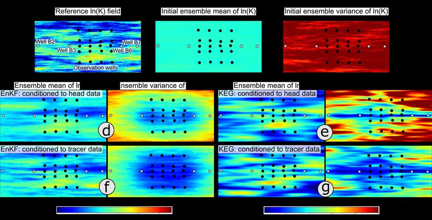
The top row of Figure 6 displays the reference log-hydraulic conductivity field (a), the initial
ensemble-mean (b), and the initial ensemble variance (c). Note that the same initial ensemble was used
in both ensemble Kalman-based methods. To facilitate a visual comparison of the parameter fields
estimated by both methods, Figure 6 also displays the ensemble-mean of log-hydraulic conductivity
and associated variance, obtained after all hydraulic-head (d ande) and tracer (f and g) data had
been assimilated. In the following, we first discuss the results of the parameter estimation based on
hydraulic-head data only, followed by those obtained after the additional assimilation of tracer data.
In both methods, the corresponding ensemble conditioned on hydraulic heads was used as the initial
ensemble in the assimilation of tracer data.
Figure 6. Top: reference log-hydraulic conductivity field (a), initial ensemble-mean of the log-hydraulic
conductivity field (b), and initial ensemble variance of log-K (c). Middle: ensemble-mean of the
log-hydraulic conductivity conditioned to all hydraulic-head data and its associated variance, estimated
with the EnKF (d) and the KEG (e). Bottom: ensemble-mean of the log-hydraulic conductivity
conditioned to all head and tracer data and its associated variance, estimated with the EnKF (f) and the
KEG (g). White dots: injection/extraction wells. Black dots: observation points.
6.1. Assimilation of Drawdown Data
A visual inspection of the log-hydraulic conductivity fields conditioned to hydraulic-head data
(Figure 6d,e) reveals that the high hydraulic conductivity zones that are located close to the pumping
and observation points, are well recovered by both methods. However, the estimation rapidly
deteriorates with distance to the observation points and pumping wells, especially for the KEG.
In general, the ensemble mean of log-hydraulic conductivity estimated with the KEG is smoother
than for the EnKF, suggesting that steady-state hydraulic head values provide less information of
small-scale variations in hydraulic conductivity than transient head data. Improvements in the
estimation of parameters with the EnKF were observed when normal-score transformations and aGeosciences 2020, 10, 276 16 of 27
damping factor were applied. We evaluated the individual effects of these tuning settings (results not
shown), but a combination of normal-score transformations and damping always outperformed the
application of only one of these settings. The best performance was achieved with a damping factor
β of 0.1. There is no clear method to define an optimal value for the damping factor β. In the EnKF,
Hendrick-Franssen and Kinzelbach [24] recommend using a value of 0.1 in groundwater problems
with mildly heterogeneous aquifers (variance of log-K close to 1). The damping factor reduces the
perturbation of the parameters in the update, improving pseudolinearizations, however, at the cost
of smoother fields. The more time-points of the hydraulic-head time series are assimilated, the more
damping is necessary, because the transient heads are strongly correlated in time. The KEG assimilates
only steady-state hydraulic heads, therefore damping is not applicable.
The mean absolute error (MAE) of the ensemble-average of the log-hydraulic conductivity field
was reduced by ~17% with the EnKF, whereas the same error metric increased by 2% with the KEG
(Table 3). We attribute the latter increase to the disagreement between reference and estimated
parameters furthest from the pumping wells and observation points. The ensemble spread quantified
by the mean ensemble standard deviation (MESD) was reduced by 30% and 16% with the EnKF
and KEG, respectively. Small ensemble spreads are not necessarily a sign of successful parameter
estimation and can be indicative of filter inbreeding, especially when no similar reduction of the misfit
is observed. Filter inbreeding quantified by the MESD/MAE ratio [23] yielded values of 0.92 and
0.89 for the EnKF and KEG, respectively (see Table 3). Average SSIM index values SSI M of 0.47 and
0.42 were estimated for the ensemble-mean of log-hydraulic conductivity fields obtained with the
EnKF and the KEG, respectively, confirming a better representation of the spatial structure of the
reference field with the EnKF, but also suggesting that the parameter fields updated with the KEG are
not entirely wrong, as implied by the increase of the MAE.
Table 3. Mean absolute error (MAE) of the ensemble-averaged log-K field, mean ensemble standard
deviation of log-K (MESD), MESD/MAE ratio, and ensemble-averaged structural similarity index
(SSIM) estimated after the assimilation of hydraulic data from pumping tests A and B. EnKF: ensemble
Kalman filter. KEG: Kalman ensemble generator.
MAE ln(K) MESD ln(K) MESD/MAE SSI M
Method (K in ms−1 ) (K in ms−1 ) (–) (–)
initial 0.73 0.79 1.08 1.0
EnKF 0.61 0.56 0.92 0.47
KEG 0.75 0.67 0.89 0.42
The spatial distribution of the ensemble spread for each method is also shown in Figure 6.
In the EnKF, the variance was smoothly reduced within the most sensitive region of the domain
(i.e., where data is available). By contrast, the KEG only partially achieved a variance reduction in the
area enclosed by the pumping wells and observation points, with a rapid increase of the estimation
variance with distance from the observation points.
Figure 7 shows scatterplots of the ensemble-mean and spread of simulated drawdown versus the
reference values computed at all observation points, for pumping tests A (Figure 7a) and B (Figure 7b).
The transient drawdown records used by the EnKF are shown as black crosses and the steady-state
values used by the KEG as red squares. To compare the performance of both methods at the end
of the parameter updates, the blue squares in Figure 7 show the drawdown values simulated at the
last assimilation time-step with the EnKF, which correspond to the steady-state drawdown values.
The ensemble spread in the transient data is shown only for the last assimilation step (blue lines).
The estimated root mean square errors were computed for the full transient data in the EnKF, and the
steady-state hydraulic heads at the last KEG assimilation iteration.Geosciences 2020, 10, 276 17 of 27
Figure 7. Calibration plot for the assimilated transient drawdown of pumping tests A (a) and B (b) used
with the EnKF (black crosses), and the steady-state drawdown for the last update iteration with the
KEG. Blue squares correspond to the last assimilation time-step with the EnKF. RMSE: root mean
square errors. Red and blue bars represent the ensemble spread of drawdown simulations.
During the assimilation of data from pumping test A, the steady-state drawdown is better
reproduced by the parameter ensemble of the KEG, despite the fewer details of the reference field
recovered. If the purpose of the data assimilation is to improve model predictions, these results alone
would suggest that no real advantage of the full transient records exist over the steady-state values.
However, the parameter ensemble of the EnKF showed less filter inbreeding issues, and a gradual
improvement in the predictions was observed after transient data of pumping test B were included.
The root mean square errors of the predicted drawdown of pumping test A are larger in the EnKF
(~150 mm) than in the KEG (9 mm), but are largely influenced by the misfit observed during the
assimilation of early-time drawdown. A considerable reduction is achieved after using data from
pumping test B, with RMSE of ~3 mm and ~2 mm for the EnKF and KEG, respectively, which are values
close to the assumed measurement error of 1 mm. Biased estimates in drawdown of pumping test
A were observed in the EnKF, in which simulated drawdown was mostly underestimated. This bias
was corrected to some degree at the end of the assimilation of the drawdown data of pumping test B
(blue points in Figure 7b), where the reference values are covered by the ensemble spread (blue lines in
Figure 7b).
These results illustrate the importance of the information contained in transient records.
Although computationally more demanding, transient data provide valuable information about aquifer
heterogeneity, that is missed if data assimilation is based only on steady-state values. Furthermore,
aquifer storativity can be incorporated in the estimation only if transient data are included. The latter
is important in real applications with transient forcings, in which aquifer storativity is uncertain.
As alternative to assimilating full transient drawdown records, temporal moments could be used.
The temporal moment-generating equations are steady-state equations with distributed source terms
depending on lower-order moments [14].
6.2. Sequential Assimilation of Concentration Data
The bottom row in Figure 6 shows the estimated ensemble mean and associated variance of
log-hydraulic conductivity after tracer data had been assimilated with the EnKF ( Figure 6f) and the
KEG ( Figure 6g). The corresponding initial ensemble mean of log-hydraulic conductivity, that is,
those conditioned to drawdown data, are presented in the middle row of Figure 6.
In general, accounting for tracer data helps refining the spatial structure of the parameter fields.
For the EnKF, an improvement of the ensemble mean of log-hydraulic conductivity could be observedGeosciences 2020, 10, 276 18 of 27
close to the observation wells, where some of the erroneous low hydraulic conductivity values obtained
with the head data were corrected. However, differences between the reference and estimated fields
outside this region were amplified, affecting the performance metrics, i.e., an increase of the mean
absolute error of log-hydraulic conductivity and a decrease in the average structural similarity index
(see Table 4). The reduction in the ensemble variance was not constrained to the region where data is
available, indicating some degree of filter inbreeding. This is quantitatively confirmed by the estimated
MESD and MAE values of 0.46 and 0.62, respectively, yielding an MESD/MAE ratio for the EnKF
of 0.74.
Table 4. Mean absolute error (MAE) of the ensemble-averaged log-K field, mean ensemble standard
deviation of log-K (MESD), MESD/MAE ratio, and ensemble-averaged structural similarity index
(SSIM) estimated after the assimilation the tracer data from tracer tests A and B. EnKF: ensemble
Kalman filter. KEG: Kalman ensemble generator.
MAE ln(K) MESD ln(K) MESD/MAE SSI M
Method (K in ms−1 ) (K in ms−1 ) (–) (–)
initial 0.73 0.79 1.08 1.0
EnKF 0.62 0.46 0.74 0.43
KEG 0.78 0.48 0.61 0.40
To reduce filter inbreeding and prevent the appearance of extreme parameter values, a stronger
damping could be applied, but this would also prevent relevant changes in the parameters and
predictions of the simulated observations. In that case, to achieve relevant improvements in the
estimation of parameters, more informative data would be required. In real-world applications,
additional data could be provided by performing more tracer tests, with the injection and extraction
of a tracer solution at different locations. An alternative to a strong damping is to increase the
ensemble size. Better approximations of the numerical covariances are obtained with larger ensembles,
and therefore the impact of the damping factor becomes less crucial. The ensemble size, however,
is constrained by the high computational costs required for transient transport simulations. To further
improve the numerical covariances, localization methods may be applied, in which covariances are
computed considering only those parameters that are located in regions believed to be sensitive to
the data.
Stronger changes could be observed in the ensemble of parameters of the KEG, which were
conditioned to the mean tracer arrival times. Some of the small-scale features of the reference field
that were missing after the assimilation of hydraulic-head data are better resolved (Figure 6g) after
assimilating the mean tracer travel times, especially in the region covered by the observation wells.
It is noticeable that the erroneous zone of low hydraulic conductivity developed below the extraction
wells B6 and B7 during the assimilation of hydraulic-head data is accentuated in the ensemble mean of
log-hydraulic conductivity conditioned to all tracer data. An elongated zone with a strong reduction
of the ensemble variance aligns with the injection and extraction wells, and extends all along the y-axis.
This behavior has been reported in previous estimations of aquifer parameters based on synthetic
tomographic tracer-tests [16], and is closely related to the distinct sensitivity of tracer arrival times on
log-hydraulic conductivity [11,12].
We observed a stronger reduction of the ensemble variance in the KEG than in the EnKF,
yielding an MESD/MAE ratio of 0.61 (Table 4). The MESD and MAE metrics are affected mainly by the
spurious parameter estimates outside the region covered by the observation wells. A decrease in the
SSI M from 0.42 after assimilation of hydraulic data, to 0.40 after using the mean tracer arrival times,
suggests that the spatial structure of the ensemble mean of parameters has been slightly deteriorated;
however, as for the MESD and MAE, this metric is strongly affected by the wrong estimations outside
the region covered by the observation wells.You can also read