The impact of hydrological model structure on the simulation of extreme runoff events - Recent
←
→
Page content transcription
If your browser does not render page correctly, please read the page content below
Nat. Hazards Earth Syst. Sci., 21, 961–976, 2021
https://doi.org/10.5194/nhess-21-961-2021
© Author(s) 2021. This work is distributed under
the Creative Commons Attribution 4.0 License.

The impact of hydrological model structure
on the simulation of extreme runoff events
Gijs van Kempen1 , Karin van der Wiel2 , and Lieke Anna Melsen1
1 Hydrology   and Quantitative Water Management, Wageningen University, Wageningen, the Netherlands
2 Royal   Netherlands Meteorological Institute (KNMI), De Bilt, the Netherlands

Correspondence: Lieke Anna Melsen (lieke.melsen@wur.nl)

Received: 8 May 2020 – Discussion started: 14 July 2020
Revised: 21 December 2020 – Accepted: 3 January 2021 – Published: 12 March 2021

Abstract. Hydrological extremes affect societies and ecosys-     etal and economic impacts. On the global scale, fatalities
tems around the world in many ways, stressing the need to        and economic losses related to high-flow events have in-
make reliable predictions using hydrological models. How-        creased dramatically over the past decades (Di Baldassarre
ever, several different hydrological models can be selected to   et al., 2010; Winsemius et al., 2016), among others due to
simulate extreme events. A difference in hydrological model      an increase in settlements in flood-prone regions. The im-
structure results in a spread in the simulation of extreme       pacts of low-flow events can be recognised in among others
runoff events. We investigated the impact of different model     the water supply, crop production and the hydropower sec-
structures on the magnitude and timing of simulated extreme      tors (Van Loon, 2015). To mitigate the societal impact of hy-
high- and low-flow events by combining two state-of-the-         drological extremes, knowledge of the processes leading to
art approaches: a modular modelling framework (FUSE) and         these extreme events is vital. Hydrological modelling is one
large ensemble meteorological simulations. This combina-         of the main tools in this quest for knowledge but comes with
tion of methods created the opportunity to isolate the impact    uncertainties. Here we aim to investigate the impact of hy-
of specific hydrological process formulations at long return     drological model structure on the magnitude and timing of
periods without relying on statistical models. We showed that    simulated extreme runoff events.
the impact of hydrological model structure was larger for           Hydrological mitigation efforts often relate to the return
the simulation of low-flow compared to high-flow events and      period of the extreme event, a measure that describes the “ex-
varied between the four evaluated climate zones. In cold and     tremeness” of the events. It is a traditional method to relate
temperate climate zones, the magnitude and timing of ex-         the magnitude of an event to the probability of occurrence
treme runoff events were significantly affected by different     of the event (Gumbel, 1941; Salas and Obeysekera, 2014),
parameter sets and hydrological process formulations, such       based on which decision makers can define their policy. Fre-
as evaporation. In the arid and tropical climate zones, the      quency analysis of extremes aims at estimating runoff levels
impact of hydrological model structures on extreme runoff        corresponding to certain return periods (Laio et al., 2009).
events was smaller. This novel combination of approaches         However, the limited length of available observational hy-
provided insights into the importance of specific hydrolog-      drological records means we rely on statistical models to es-
ical process formulations in different climate zones, which      timate return periods most of the time (Meigh et al., 1997;
can support adequate model selection for the simulation of       Michele and Rosso, 2001; Smith et al., 2015; Sousa et al.,
extreme runoff events.                                           2011), e.g. by fitting a generalised extreme value (GEV) dis-
                                                                 tribution.
                                                                    Despite the wide application of GEV analysis to relate
1   Introduction                                                 runoff to return periods, there are some important caveats to
                                                                 this method. The statistical models are particularly used for
Extreme high- and low-flow events, often referred to as          extrapolation – to estimate the probability of yet unobserved
floods and droughts, respectively, have high natural, soci-

Published by Copernicus Publications on behalf of the European Geosciences Union.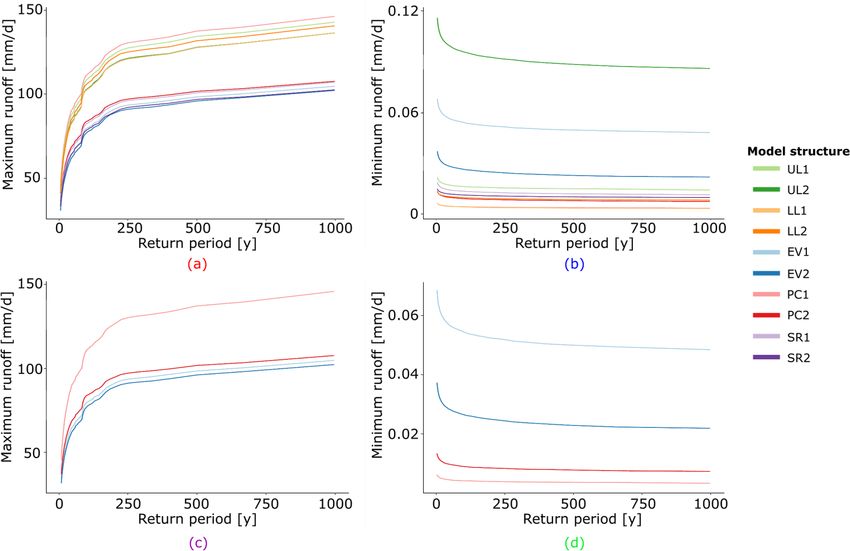
962                                                  G. van Kempen etal.: The impact of model structure on extreme events

extremes. As such, the projected hydrological extremes are         ble meteorological simulations. The forcing data set consists
highly sensitive to small changes in the parameters of statis-     of 2000 years of daily meteorological data, representing the
tical models (Engeland et al., 2004; Smith et al., 2015; Kle-      present-day climate conditions. This data set will be used to
meš, 2000), leading to distributions that might substantially      force several hydrological models within the FUSE frame-
change when a single data point is added (see e.g. Brauer          work. The different model structures will be used to evalu-
et al., 2011). Furthermore, the physical processes leading to      ate various hydrological process formulations, to determine
extrapolated extreme events can not be investigated. A recent      which process formulations have the largest impact on the
alternative to extreme value statistics models, proposed for       simulated magnitude and timing of extreme high- and low-
example by Van der Wiel et al. (2019), is to use large ensem-      flow events in different climate zones. Due to the length of
ble model simulations: a climate model simulates long time         the forcing time series, the extreme runoff events in the tail
series of meteorological conditions, and with a hydrological       of the distribution can be evaluated using simulated values.
model this is translated to runoff, resulting in a long time se-   Hence, we do not rely on statistical models to extrapolate
ries that does not require extrapolation for the investigation     extreme events. As such, this study contributes to the under-
of events of longer return periods.                                standing of the impact of model structural uncertainty in hy-
    In this approach, hydrological models are employed to          drological models on simulated extreme runoff events.
translate meteorological time series into hydrological time
series, from which relevant events can be selected and in-
vestigated. Uncertainty is, however, also inevitable in model      2     Methods
simulations (Oreskes et al., 1994). In hydrological mod-
elling, different sources of uncertainty can be distinguished,     We assessed the impact of hydrological model structural un-
for instance data uncertainty, parameter uncertainty and           certainty on extreme runoff events by using large ensemble
model structural uncertainty (Ajami et al., 2007). Data un-        meteorological simulations in combination with the hydro-
certainty can be related to random or systematic errors in         logical modular modelling framework FUSE. We examined
the model forcing. Parameter uncertainty can be caused by          four different climate zones because hydrological processes
sub-optimal identification of parameter values or equifinal-       vary considerably between climates (Pilgrim, 1983), which
ity, and model structural uncertainty relates to incomplete or     leads to different processes being of importance in control-
biased model structures (Butts et al., 2004). It is important      ling the extreme events (Di Baldassarre et al., 2017; Eagle-
to gain insight into the uncertainty of environmental models       son, 1986). In the R version of FUSE (Vitolo et al., 2015),
and to communicate these insights to decision makers (Liu          10 different model structures were employed, and to repre-
and Gupta, 2007), especially in the perspective of extreme         sent the complete parameter space, 100 parameter sets were
events that give rise to policy making.                            used for every model structure. The simulated extreme runoff
    Data uncertainty and parameter uncertainty can be quan-        events were compared based on their magnitude and timing.
tified by a combination of error propagation and sampling
(Li et al., 2010; McMillan et al., 2011a). The quantification      2.1    Meteorological forcing data
of model structural uncertainty is more challenging, since it
takes a considerable amount of time and effort to set up and       We employed a 2000-year time series of meteorological data,
run several model structures. Furthermore, it is difficult to      generated by the EC-Earth global coupled climate model
link intermodel differences to alterations in certain hydrolog-    (v2.3, Hazeleger et al., 2012). This 2000-year time series
ical process formulations (Clark et al., 2008), because mod-       originally consisted of a large ensemble of 400 sets of 5-year
els often differ in several process formulations. This is where    runs. In this study, these 400 sets were assumed to be one
the use of modular modelling frameworks (MMFs), a tool             long time series, which enables extensive return period anal-
which facilitates switching between model structures (Addor        ysis. This time series represents a period with a simulated
and Melsen, 2019), might provide ways forward in the evalu-        absolute global mean surface temperature (GMST) equal to
ation of model structural uncertainty. In a MMF it is possible     the observed GMST in the years 2011–2015 based on Had-
to alter a minor part of the model structure, which allows the     CRUT4 data (Morice et al., 2012). The time series thus rep-
researcher to isolate choices in the model development pro-        resents present-day climatic conditions. In Van der Wiel et al.
cess (Knoben et al., 2019). The Framework for Understand-          (2019), this data set was used to evaluate the benefits of the
ing Structural Errors (FUSE, Clark et al., 2008) is an exam-       large ensemble technique for hydrology. Further details on
ple of a modular modelling framework, which can be used to         the design of the meteorological forcing data are provided in
diagnose differences in hydrological model structures.             that paper.
    This study is designed to evaluate the impact of hydro-           The 2000-year meteorological time series as employed by
logical model structure on the magnitude and timing of sim-        Van der Wiel et al. (2019) has global coverage at 1.1◦ hori-
ulated extreme runoff events with different return periods.        zontal resolution. However, for this study we restricted our-
We combine two state-of-the-art approaches: the hydrolog-          selves to four climate zones, represented by one grid cell for
ical modular modelling framework FUSE and large ensem-             each climate zone (Fig. 1). Simulated monthly averaged 2 m

Nat. Hazards Earth Syst. Sci., 21, 961–976, 2021                                   https://doi.org/10.5194/nhess-21-961-2021
G. van Kempen etal.: The impact of model structure on extreme events                                                                    963

Figure 1. Köppen–Geiger climate map indicating the locations of the selected grid cells for the four different climate zones and their
corresponding climatology and hydrology (central map taken from Peel et al., 2007, their Fig. 10). The climate graphs show simulated cli-
matological monthly precipitation sums (blue bars) and monthly average temperatures (red lines). The hydrological conditions are visualised
using simulated monthly average runoff levels. The different line colours represent the 10 evaluated model structures, and the spread induced
by the different parameter sets is shown using grey bands.

temperatures and precipitation sums were obtained from the               2.2   Framework for Understanding Structural Errors
EC-Earth model to classify grid cells based on the Köppen–                     (FUSE)
Geiger criteria and allow the selection of appropriate grid
cells for this study. We selected four grid cells to represent           FUSE is a modular modelling framework, which can be
the arid (BWh), cold (Dfc), temperate (Cfb) and tropical                 used to diagnose differences in hydrological model structures
(Aw) climate. This set of climate zones offers a comprehen-              (Clark et al., 2008). FUSE is developed based on four par-
sive representation of the global climate zones (Kottek et al.,          ent models: the US Geological Survey’s Precipitation-Runoff
2006; Peel et al., 2007).                                                Modelling System (PRMS, Leavesley, 1984), the NWS
   Daily 2 m temperature, precipitation and potential evapo-             Sacramento model (Burnash et al., 1973), TOPMODEL
transpiration data for the full 2000 years were then acquired            (Beven and Freer, 2001) and different versions of the variable
for the four selected grid cells. The 2 m temperature and daily          infiltration capacity (ARNO/VIC) model (Liang et al., 1994).
precipitation fluxes were directly available from the EC-                This framework enables the assessment of intermodel dif-
Earth model. Potential evapotranspiration fluxes were cal-               ferences in another way compared to other model intercom-
culated following the Penman–Monteith method (Zotarelli                  parison studies (Henderson-Sellers et al., 1993; Reed et al.,
et al., 2015). The precipitation and potential evapotranspi-             2004). In FUSE, each model component can be adapted in
ration fluxes were used as input in the FUSE models; the                 isolation, and therefore the effect of specific hydrological
2 m temperature was used to force the snow module (see                   process formulations can be investigated. In the next subsec-
Sect. 2.2).                                                              tion we further discuss which model structures we selected
                                                                         and which process formulations were tested.
                                                                            All model structures used in this study were lumped hy-
                                                                         drological models, which were run at a daily time step. We
                                                                         employed a spin-up period of 5 years, before forcing the hy-

https://doi.org/10.5194/nhess-21-961-2021                                          Nat. Hazards Earth Syst. Sci., 21, 961–976, 2021
964 G. van Kempen etal.: The impact of model structure on extreme events
Table 1. The model structures that were employed in this study. Each letter refers to a specific hydrological process formulation as in Clark
et al. (2008); the model IDs are described by Vitolo et al. (2015). The model abbreviations are related to the alteration in the model structure
and are used throughout this paper.
Model component Model number
1 2 3 4 5 6 7 8 9 10
Upper layer A B C C C C A A A A
Lower layer A A A C B B B B C C
Base flow A A A B C C C C B B
Evaporation A A B B A B A A A A
Percolation C C C C C C C B B B
Interflow A A A A A A A A A A
Surface runoff A A A A B B A A A B
Routing A A A A A A A A A A
Model ID 802 800 642 626 808 652 790 880 874 896
Abbreviation UL1 UL2 LL1 LL2 EV1 EV2 PC1 PC2 SR1 SR2
Alteration Upper layer Lower layer Evaporation Percolation Surface Runoff
drological models with the 2000-year meteorological time be altered, and the process formulations for simulating base
series. The simulated monthly average runoff varied among flow, evaporation, percolation, surface runoff, interflow and
the evaluated model structures and parameter sets (Fig. 1). routing can be changed. The lower-layer architecture is inti-
Therefore, it is essential to select an adequate hydrological mately tied to the process formulation of base flow. There-
model for the simulation of runoff levels, and it will likely be fore, they need to be changed simultaneously and only a few
of larger importance when simulating extreme runoff events. combinations are possible.
FUSE as implemented in R (Vitolo et al., 2015) does Ten different model structures were evaluated in this study.
not include a snow module. However, snow storage and Table 1 provides an overview of the selected hydrological
snowmelt might be important components in the hydrologi- model structures. In the odd model numbers, new model
cal cycle of the colder climate zones. Therefore, a snow mod- structures were constructed, and in the even model numbers,
ule was implemented. First, a threshold temperature was de- a single hydrological process was altered in the model struc-
fined at 0 ◦ C, below which precipitation is assumed to fall ture relative to the preceding odd model number. By compar-
as snow. Secondly, snowmelt is simulated by using a simple ing the extreme runoff events simulated between consecutive
degree-day method (Kustas et al., 1994): odd- and even-numbered model structures, we analysed the
impact of a specific hydrological process on extreme event
M = a(Ta − Tb ), (1)
simulation, indicated by the alteration in Table 1.
in which M represents snowmelt (cm d−1 ), a the degree- For our synthetic experiment, we decided to apply a fixed
day factor (cm ◦ C−1 d−1 ), Ta the average daily temperature routing scheme. The effect of routing parameters on the dis-
(◦ C) and Tb the base temperature (◦ C). The range in the charge signal is delay and attenuation. As such, the main ef-
degree-day factor is between 0.35 and 0.60 under most cir- fect of the routing scheme would be to decrease the peak
cumstances (Kustas et al., 1994). Therefore, the degree-day height. Since we evaluate our model results on (among oth-
factor was fixed at a value of 0.475 cm ◦ C−1 d−1 , and Tb was ers) peak height, the routing would dominate the results with-
set to 0 ◦ C. The degree-day method employed daily 2 m tem- out providing insights into the underlying runoff-generating
perature data to subdivide the precipitation data into rain and processes. Besides routing, the process formulation of inter-
snow and to determine the melt rate. The different FUSE flow was left unchanged throughout this study, as it was not
model structures were subsequently forced by these subdi- explicitly parameterised in TOPMODEL and ARNO/VIC
vided precipitation fluxes. The degree-day parameters were (Clark et al., 2008).
kept constant across the experiments because we only ex- In contrast to other studies that evaluate different model
plore one snow formulation (in contrast to the other pro- structures (Atkinson et al., 2002), this study evaluated differ-
cesses, for which model formulations were all varied). ences among model structures that are deemed to be equally
plausible. Hence, there were no prior expectations of specific
2.2.1 Selected model structures models to outperform other models. This means that the em-
phasis in FUSE is not on the lacking parts of hydrological
In total, 1248 different model structures can be constructed in
models but on the intermodel differences that are caused by
FUSE as implemented in R (Vitolo et al., 2015) by combin-
different representations of the real world (Clark et al., 2008).
ing different hydrological process formulations from the par-
ent models. The architecture of the upper and lower layer can
Nat. Hazards Earth Syst. Sci., 21, 961–976, 2021 https://doi.org/10.5194/nhess-21-961-2021G. van Kempen etal.: The impact of model structure on extreme events 965
Figure 2. D statistics for maximum (a) and minimum (b) runoff in one model structure (UL1) with 12 parameters, which result from the
Kolmogorov–Smirnov test. The other model structures show a similar trend (not shown). The bands are a result of the different parameter
samples; the different colours represent the four climate zones.
2.2.2 Parameters rameter ranges provided by Vitolo et al. (2015), as given in
Table 2.
In this synthetic experiment, the parameters of the hydrolog-
ical models were not calibrated to real catchment observa- 2.3 Magnitude of extreme runoff events
tions. Instead, the parameters of the models were sampled
over their full range. Since in calibrated experiments it is al- The magnitudes of the simulated extreme events were eval-
ways difficult to differentiate the effect of parameter values uated by comparing the distribution of runoff values based
from the effect of model structure, the parameter sampling on four return periods: 25, 50, 100 and 500 years. The as-
approach also created the opportunity to assign the effect on sociated runoff levels were determined by sorting the time
extreme events either to parameter values or to model struc- series of annual maximum and minimum daily runoff values.
ture. This resulted in 2000 sorted runoff values from which events
To investigate the appropriate and feasible number of were selected. For instance, for the 500-year return period,
parameter sets required to sufficiently capture parame- the fourth most extreme value in the sorted time series was
ter space, the Kolmogorov–Smirnov test was employed taken.
(Massey, 1951). With the Kolmogorov–Smirnov test, we The different model structures yielded different simulated
compare the difference in the distribution of the hydrolog- magnitudes for extreme runoff events (Fig. 3a). Every model
ical model output between a small parameter sample and structure was run using 100 different parameter sets, which
a large benchmark sample. Our benchmark sample had a led to bands around the projected extreme runoff events
size of 5000 parameter sets. We applied the Kolmogorov– (Fig. 3b). The runoff values and their bands were subse-
Smirnov test to assess the annual maximum and minimum quently evaluated for 25-, 50-, 100- and 500-year return pe-
daily runoff from 10 up to 200 parameter sets, each time riods (Fig. 3c). The different parameter sets resulted in 100
with a 10-sample increment. The model runs were exe- extreme runoff values at a specific return period for every
cuted for 30 years to save computation time, because this model structure. In order to test whether the projected differ-
is considered sufficient to represent the mean climate con- ence in the distributions of these runoff values (Fig. 3d) was
ditions (McMichael et al., 2004). The D statistic describes significantly different from the paired model, a two-sample
the largest distance between the empirical cumulative dis- t test was applied. This test was used to evaluate related
tribution functions (ECDFs), which indicates that when the model structures based on a change in one single hydro-
D statistic decreases, the ECDFs are more likely to originate logical process formulation (Table 1). By comparing related
from the same data set. model structures, the impact of corresponding hydrological
We found that the optimal trade-off between computer process formulations could be isolated for specific climate
time and sufficiently capturing parameter space was at zones and return periods.
100 parameter sets, as the D statistic stabilised at this value For the magnitude analysis of low-flow events, we encoun-
(Fig. 2). Since there are different process formulations, the tered that some combinations of model structures and pa-
number of sampled parameters varied between 11 and 15 for rameter sets led to a very low fixed value (in the order of
the different model structures. Nevertheless, for justification 10−4 and less), which we refer to as hard-coded lower limits.
we used 100 parameter sets for all model structures, indepen- These lower limits varied between model structures, depend-
dent of the number of parameters. The parameter sets were ing on the configuration of different storage reservoirs. These
generated using Latin hypercube sampling, based on the pa- limits assure numerical stability but could obfuscate our anal-
https://doi.org/10.5194/nhess-21-961-2021 Nat. Hazards Earth Syst. Sci., 21, 961–976, 2021966 G. van Kempen etal.: The impact of model structure on extreme events
Table 2. Description and range of the parameters that were sampled, based on Vitolo et al. (2015)
Parameter Description Unit Values
Min Max
rferradd additive rainfall error mm 0 0
rferrmlt multiplicative rainfall error – 1 1
frchzne fraction tension storage in recharge zone – 0.05 0.95
fracten fraction total storage in tension storage – 0.05 0.95
maxwatr1 depth of the upper soil layer mm 25 500
percfrac fraction of percolation to tension storage – 0.05 0.95
fprimqb fraction storage in first baseflow reservoir – 0.05 0.95
qbrate2a baseflow depletion rate first reservoir d−1 0.001 0.25
qbrate2b the baseflow depletion rate second reservoir d−1 0.001 0.25
qbprms baseflow depletion rate d−1 0.001 0.25
maxwatr2 depth of the lower soil layer mm 50 5000
baserte baseflow rate mm d−1 0.001 1000
rtfrac1 fraction of roots in the upper layer – 0.05 0.95
percrte percolation rate mm d−1 0.01 1000
percexp percolation exponent – 1 20
sacpmlt SAC model percolation multiplier for dry soil layer – 1 250
sacpexp SAC model percolation exponent for dry soil layer – 1 5
iflwrte interflow rate mm d−1 0.01 1000
axvbexp ARNO/VIC b exponent – 0.0001 3
sareamax maximum saturated area – 0.05 0.95
loglamb mean value of the topographic index m 5 10
tishape shape parameter for the topographic index gamma distribution – 2 5
qbpowr baseflow exponent – 1 10
timedelay time delay in runoff d 2.5 2.5
Figure 3. Illustration of the conducted procedure for the comparison of the extreme event magnitude. The four lines with different colours
represent the different model structures (theoretical structure 1–4). (a) The simulated runoff can be plotted against return period for the
different models. (b) The uncertainty bounds are due to the 100 different parameter samples per model. (c) The parameter samples were
compared at different return periods. (d) The projected difference between the distributions at a given return period of the various model
structures was tested using a two-sample t test; an example of a significant and a not-significant difference is shown.
ysis because the difference between distributions simulating to evaluate the timing of the 500-year events based on the
lower limits would be significant if the lower limits between entire 2000-year time series. Extreme hydrological events do
two model structures had different values. Conceptually, the not always result from extreme meteorological conditions but
lower limits represent zero discharge: the river has run dry. could also originate from a sequence of moderate weather
As such, no significant difference should be found when two conditions (Van der Wiel et al., 2020). By assessing the tim-
models reached this lower limit. Therefore, in all simulations ing of extreme runoff events, we investigated whether the
the lower limit in discharge was set equal to zero. timing of the extreme runoff events is controlled by differ-
ent model structures and parameter sets or determined by the
2.4 Timing of extreme runoff events meteorological forcing.
An asset from the ensemble approach for return period eval-
uation compared to GEV statistics is that it also allows us
Nat. Hazards Earth Syst. Sci., 21, 961–976, 2021 https://doi.org/10.5194/nhess-21-961-2021G. van Kempen etal.: The impact of model structure on extreme events 967 Figure 4. Illustration of the procedure for the comparison of the timing of extreme events, equal to or greater than 500-year events. (a) In each simulation, the monthly maximum daily runoff (MMDR) values were sorted and the four most extreme events were selected (green cells); this table shows an example for one parameter set. (b) All parameter sets of one model structure were concatenated, and the sum (red cells) indicated the variation in timing in one model structure. A score of 100 means that for all different parameter sets, the same event is selected. (c) All model structures of one climate zone were concatenated, and the sum (blue cells) indicated the variation in extreme event timing in all model structures for one climate zone. The values in the blue cells have a maximum score of 1000 (10 models, with 100 parameter samples each). A score of 1000 indicates that all models and all parameter sets identify the same event as a 500-year event (100 % model agreement). Given that we have 2000 years of simulations and evaluate 500-year events, the ideal case where all models agree would result in four events with a score of 1000. (d) Stacked bar charts are used to visualise the model agreement of specific runoff events. Each row in panel (c) represents one colour in the coloured bars in panel (d); the total height of each bar is determined by the value in the blue cells in panel (c). Grey shading behind the bars indicates the theoretical maximum for 500-year events: four runoff events with 100 % model agreement. The timing of extreme runoff events with 500-year return rameter values. For instance, in Fig. 4d, one event is iden- periods was compared. This was done in four steps, as de- tified by almost all simulations, and it approaches a fully picted in Fig. 4. coloured bar chart. The percentage of model agreement was First, we sorted all the monthly maxima and minima determined by the number of model simulations that identify daily runoff values and their corresponding simulation month a specific extreme runoff event out of a total of 1000 model (Fig. 4a). The four most extreme events in this sorted 2000- simulations, where all model simulations employed a unique year data set represent the extreme events equal to or greater combination of a model structure and a corresponding pa- than the 500-year events. These four most extreme events rameter set. were determined for each model simulation, so for each com- If all combinations of different model structures and pa- bination of model structure and parameter sets. rameter sets were to agree upon the timing of this extreme Then, we evaluated to what extent the same events were event, only four events would be identified in total. This selected for different parameter sets, but with the same model would lead to the theoretical maximum, where there are four structure. If one event were for instance selected for all 100 fully filled stacked bar charts and an x axis going to a maxi- parameter sets, this particular event would have a score of mum of four. This would be shown by four fully stacked bar 100 in the red row of Fig. 4b. If this event were only selected charts, in other graphs shown by grey shading. When the sim- for half of the parameter sets, it would have a score of 50. If ulations do not agree upon the timing, there will be more bars across all parameter sets the same four events were identified, in the chart, indicating the variation in the timing. The value this would result in four times a score of 100 in Fig. 4b. This of the x axis indicates the total number of selected extreme indicates that the influence of hydrological parameters on the events. For example, a value of 20 on the x axis indicates timing of the extreme event is negligible. that across all simulations 20 different 500-year events with This procedure was repeated across all 10 model struc- a different timing were identified. We sort the selected events tures. If the same event were selected for all parameter sets by model agreement, with events of bigger model agreement (n = 100) and for all models (n = 10), it would result in a (higher bars) shown on the right. score of 1000 in the blue row of Fig. 4c. If the same four events were selected across all models and all parameter sets, four times a score of 1000 would be found. In that case, both 3 Results model structure and model parameters have negligible influ- ence of the timing of the extreme event: the event is mainly 3.1 Magnitude of extreme runoff events triggered by meteorological circumstances. Finally, the model agreement of the specific extreme This section describes the impact of model structures on ex- runoff events was evaluated in stacked bar charts (Fig. 4d). treme event magnitude for different climate zones, hydrolog- The colours of the stacked bars represent the different model ical process formulations and return periods. We compared structures, and the height of these bars indicates the model the distribution of the magnitudes of the extreme high- and agreement within a specific model structure for different pa- low-flow events for related model structures, based on four https://doi.org/10.5194/nhess-21-961-2021 Nat. Hazards Earth Syst. Sci., 21, 961–976, 2021
968                                                     G. van Kempen etal.: The impact of model structure on extreme events

Figure 5. The ensemble mean of the annual maximum (a, c) and minimum (b, d) daily runoff levels at different return periods in the tropical
climate zone. The ensemble mean is obtained based on 100 parameter sets. In panels (a) and (b) all model structures are visualised. In panels
(c) and (d), a selection of only four model structures is presented to emphasise the difference between the model structures. These four model
structures are related by alterations in the evaporation (EV1, EV2) and percolation (PC1, PC2) process formulations (Table 1). The colours
of the panel labels refer to the boxes of the same colours in Fig. 6.

different return periods, and for four different climate zones.             An alteration in the model structure has significant impact
Alterations in the hydrological process formulations lead to             in about a quarter of the model output comparisons during
a difference in the magnitude of extreme runoff events, as               high-flow events (Fig. 6a). The difference between the mag-
depicted in Fig. 3a, which is an example showing the prin-               nitude distributions of the high-flow events is non-significant
ciple. Figure 5 shows the same information but based on ac-              for alterations in the architecture of the upper and lower layer
tual simulations of high flows (Fig. 5a and c) and low flows             and in the process formulation of surface runoff. This means
(Fig. 5b and d) in the tropical climate zone. We then em-                that the magnitude of high-flow events for all climate zones
ployed a two-sample t test to calculate the p values (Fig. 6),           and return periods is not sensitive to changes in the formula-
which were used to distinguish the statistically significant             tion of these hydrological processes.
(p ≤ 0.05) and non-significant (p > 0.05) differences in the                In the arid climate zone, the impact of alterations in model
distribution of extreme event magnitudes as in Fig. 3d.                  structures on high-flow events has the least impact. This indi-
   Panels (c) and (d) of Fig. 5 highlight four models in the             cates that the magnitudes of the high-flow events are mainly
tropical climate zone for comparison. The model structures               controlled by the meteorological forcing. In the cold and tem-
that are related by an alteration in the process formulation of          perate climate zones, the high-flow events are sensitive to al-
percolation simulate a difference in extreme high-flow mag-              terations in the process formulation of two hydrological pro-
nitude for all return periods (red lines in Fig. 5c). Based on           cesses: evaporation and percolation. This indicates that the
the t test conducted on these distributions, this results in a           magnitudes of the high-flow events are not only determined
significant impact of alterations in the process formulation             by the meteorological forcing, but there is also a notable im-
of percolation for all return periods (as displayed in Fig. 6).          pact of the hydrological model structure, specifically for the
In contrast, the model structures related by an alteration in            formulation of these two processes. Finally, in the tropical
the process formulation of evaporation simulate comparable               climate zone, the high-flow events are only sensitive to al-
runoff values across all return periods for high flows (blue             terations in the process formulation of percolation. The other
lines in Fig. 5c). Therefore, there is no significant impact on          hydrological process formulations do not significantly affect
the magnitude of extreme high-flow events caused by this                 the magnitude of high-flow events in this climate zone.
hydrological process formulation (Fig. 6). For the low flows,               For low-flow events, the model structure has a greater im-
an alteration in the percolation formulation (Fig. 5d) does              pact on the simulation of extreme events. An alteration in the
not lead to statistically significant differences in the low-flow        model structure has significant impact in half of the model
distribution (Fig. 6), whereas an alteration in the evaporation          output comparisons during low-flow events (Fig. 6b). In the
formulation leads to a difference at the 0.1 significance level.         arid climate zone, the low-flow events are sensitive to alter-

Nat. Hazards Earth Syst. Sci., 21, 961–976, 2021                                            https://doi.org/10.5194/nhess-21-961-2021
G. van Kempen etal.: The impact of model structure on extreme events                                                                        969

Figure 6. Statistically significant (p ≤ 0.05) and non-significant (p > 0.05) differences between the distribution of magnitudes for extreme
runoff events, assessed by a two-sample t test. The colours indicate whether an alteration in the model structure has a statistically significant
impact on the magnitude of extreme high- (a) and low-flow (b) events. This is shown for the four climate zones (arid, cold, temperate and
tropical, indicated at the top) and the four different return periods (25, 50, 100 and 500 years). The red values in panel (b) indicate the
percentage of simulations which reached zero runoff conditions (dry river). The coloured boxes refer to the results displayed in the panels of
Fig. 5.

ations in the architecture of the upper and lower layer. In                agreement on the timing of extreme high-flow events with a
the cold and temperate climate zones, the low-flow events                  return period equal to or greater than 500 years, as earlier
are also sensitive to alterations in the architecture of the up-           depicted in Fig. 4d. For the low-flow events, the timing eval-
per and lower layer and additionally to changes in the pro-                uation could not be conducted, because of the nature of low-
cess formulation of evaporation. In the tropical climate zone,             flow events to persist longer. This will be further discussed
the low-flow events are less sensitive to alterations in the ar-           in this section.
chitecture of the lower layer and the process formulation of                  The impact of different hydrological process formulations
evaporation but still sensitive to alterations in the upper-layer          and parameter sets on the timing of extreme high-flow events
architecture. In most climate zones, changing the formulation              varies between the selected climate zones. In the arid and
of multiple hydrological processes significantly impacts the               tropical climate zones, there are multiple events with a model
simulation of the magnitude of low-flow events, which im-                  agreement exceeding 99 %. In these cases, almost all model
plies that the model structure is an important source of uncer-            simulations agree on the timing of these extreme events. Just
tainty. The meteorological forcing is clearly not the only fac-            10 and 8 runoff events were selected (out of a total of 24 000
tor controlling the magnitude of simulated low-flow events.                potential events) as extreme high-flow events in the arid and
   A phenomenon that does play an important role in the eval-              tropical climate zones, respectively (Fig. 7). This means that
uation of low flows is that eventually in some cases the sim-              there are only a few model simulations that deviate by sim-
ulated runoff goes to zero, indicating that no more water is               ulating the most extreme runoff events at a different point
flowing through the river. For instance, in the arid climate               in the time series. For these climate zones, this implies that
zone, for the two models where percolation is altered, 100 %               the timing is mainly prescribed by the meteorological forc-
of the simulations have zero discharge already for the 25-                 ing. This might be explained by the precipitation climatology
year return period events. Differences in low flows as a con-              in these climate zones. On average, in the arid climate zone
sequence of changing the percolation formulation can then                  the daily precipitation sum exceeds 1 mm only during 11 d
no longer be traced and thus do not lead to a significant dif-             a year. Precipitation is therefore scarce and characterised by
ference.                                                                   short events of high intensity (Goodrich et al., 1995), which
                                                                           propagate into extreme runoff events. In the tropical climate
3.2   Timing of extreme runoff events                                      zone, there is a high precipitation rate throughout the com-
                                                                           plete time series. However, there is a pronounced wet season
The timing of extreme high-flow events is evaluated using                  from October until April (Fig. 1). There are multiple extreme
stacked bar charts. Figure 7 shows the percentage of model                 precipitation events larger than 150 mm d−1 . The 500-year

https://doi.org/10.5194/nhess-21-961-2021                                             Nat. Hazards Earth Syst. Sci., 21, 961–976, 2021
970 G. van Kempen etal.: The impact of model structure on extreme events Figure 7. Stacked bar charts that visualise the percentage of model agreement for extreme high-flow events. Four different climate zones are evaluated in the different subplots: arid (a), cold (b), temperate (c) and tropical (d). Extreme runoff events are identified when they are equal to or greater than the 500-year return level. The linked model structures (Table 1) are related to each other by comparable colours. Grey shading indicates the theoretical maximum of four events with 100 % model agreement, which would imply a negligible impact of model structure and parameters on high-flow event timing. extreme runoff events are initiated by these extreme precipi- riods, and therefore it was not possible to select the four tation events. most extreme events. This invalidates our method to inves- In both the cold and temperate climate zone, there is only tigate the impact of different model structures on the timing one event with a model agreement exceeding 99 % (Fig. 7). of low-flow events, at least with the definition of low-flow In the cold and temperate climate zones, there are 20 and 38 events as we employ it (directly evaluating the runoff). Zero different events selected as extreme events, respectively. The runoff, representing a dry river, mostly occurs in the drier cli- selected runoff events with the highest model agreement are mate zones. In the arid climate zone, the runoff levels drop to initiated by the most extreme precipitation events, whereas zero in 69 % of all the model simulations. In the cold climate the selected extreme runoff events with a low model agree- zone, 53 % of the model combinations simulate zero runoff. ment are most likely initiated by compound events (Van der In this climate zone, the temperature regularly drops below Wiel et al., 2020; Zscheischler et al., 2018). Hence, the tim- 0 ◦ C (Fig. 1), which indicates that precipitation falls as snow ing of extreme high-flow events may depend more on hydro- instead of rain. This transition affects the runoff-generating logical processes and consequently vary across hydrological processes (Immerzeel et al., 2009), which results in lower model structures and parameter values in these climate zones. runoff levels during colder periods (Fig. 1). In the temper- The stacked bar charts indicate which model structures lead ate and tropical climate zones, 39 % and 36 %, respectively, to the selection of events with low agreement. Some model of all combinations of model structures and parameter sets structures seem to show deviant behaviour, but there is no simulate zero runoff. convincing pattern visible; most model structures seem to be represented in low-agreement events. Therefore, there is no clear relationship between the extreme runoff events with a 4 Discussion low model agreement and specific model structures. We hy- pothesise that this uncertainty can be assigned to the differ- This study evaluates the spread introduced by different hy- ence in parameter sets. drological model structures and parameters on the magnitude To evaluate the timing of extreme low-flow events, a sim- and timing of simulated extreme runoff events. Both differ- ilar approach was applied compared to the high-flow events. ences and similarities can be identified between the distri- However, for several combinations of model structures and butions of runoff values for the high- and low-flow events. parameter sets, zero runoff was simulated (Fig. 5b). These Alterations in hydrological model structures more often re- periods of zero runoff often persisted for longer time pe- sult in significant differences in low flows (45 %) compared Nat. Hazards Earth Syst. Sci., 21, 961–976, 2021 https://doi.org/10.5194/nhess-21-961-2021
G. van Kempen etal.: The impact of model structure on extreme events                                                          971

to high flows (24 %), which implies a larger model structural      4.1   Climate synthesis
uncertainty in the magnitude of low-flow events. High-flow
events mainly depend on precipitation, i.e. meteorological         The magnitude and timing of the extreme high-flow events
forcing, while the influence of other runoff-generating pro-       in the arid climate zone are mainly controlled by the me-
cesses such as soil moisture and base flow is marginal (Zhang      teorological forcing. This is contrary to previous studies in
et al., 2011). This is not to say that these processes are not     which the runoff in dry catchments was more sensitive to
relevant: merely, our results demonstrate that the way these       different hydrological models (Jones et al., 2006; Lidén and
processes are formulated in the model has limited impact on        Harlin, 2000), but here we specifically refer to high-flow
the model result. The situation during high-flow events is of-     events in arid climates. In this climate zone, precipitation is
ten characterised by a precipitation surplus. Therefore, there     scarce and often characterised by extremely variable, high-
will be more or less continuous groundwater recharge by per-       intensity and short-duration events (Goodrich et al., 1995).
colation in the unsaturated zone (Knutsson, 1988), which ex-       Consequently, runoff in arid climate zones is characterised
plains why the formulation of percolation appears as a rele-       by a dominance of Hortonian overland flow (Segond et al.,
vant hydrological process to estimate the magnitude of high-       2007). This runoff-generating process is not included in the
flow events.                                                       implementation of FUSE, which might reduce the impact of
   Hydrological models are traditionally designed to simu-         different model structures (Clark et al., 2008). Also the tem-
late the runoff response to rainfall, and therefore it seems to    poral resolution at which we ran the model and evaluated the
be more challenging to simulate low-flow events (Staudinger        high-flow events might be relevant. The extremely flashy pre-
et al., 2011). The low-flow events are mainly sensitive to         cipitation patterns can cause flash floods that occur over the
alterations in the architecture of the upper and lower layer.      course of a few hours. We evaluate the model results at the
Earlier research indicates the importance of the lower-layer       daily time step, which can cover up the occurrence of flash
architecture and the process formulation of base flow in sim-      flood events. For the low-flow events, we found more spread
ulating low-flow events (Staudinger et al., 2011). The archi-      in the magnitude as a consequence of altering process formu-
tecture of the upper and lower layer defines the water content     lations. Alterations in multiple hydrological processes result
in these layers (Clark et al., 2008). This water content con-      in significant differences.
trols the runoff-generating processes during low-flow events          In the cold and temperate climate zones, there is more
due to a precipitation deficit and reduces the importance of       spread in the simulations regarding the magnitude and tim-
the percolation process (Andersen et al., 1992). Therefore,        ing of extreme runoff events. The magnitudes of extreme
alterations in the process formulation of percolation mainly       high- and low-flow events are sensitive to alterations in mul-
affect high-flow events in the wet climate zones. Alterations      tiple hydrological process formulations, which implies that
in model structures have no distinct impact on the simulated       several hydrological processes are important in the runoff-
timing of high-flow events. Nevertheless, there is a spread in     generating processes in these climate zones, as also discussed
the timing of these events, which is most likely caused by the     by Scherrer and Naef (2003). In different model simulations,
difference in parameter sets.                                      different high-flow events are identified as the most extreme
   Besides these differences, there are also similarities in the   runoff events, which leads to a spread in the timing of these
simulation of high- and low-flow events. The magnitudes of         events. This spread is partly assigned to the difference in pa-
high- and low-flow events in the cold and temperate climate        rameter sets.
zone show significant differences for the same alterations            We only tested a limited number of processes and pro-
in the hydrological process formulations. Furthermore, al-         cess formulations. However, especially in the cold and tem-
terations in the process formulation of surface runoff have        perature climate zones, extreme events related to snowmelt
no significant impact on the magnitude of both types of ex-        can potentially occur. Therefore, the process formulation of
treme runoff events. This might be due to the lacking im-          snowmelt could have significant impact on the simulations.
plementation of infiltration excess overland flow in FUSE          This was, however, not tested because we only used a sin-
(Clark et al., 2008). This could be an important factor for        gle degree-day snow formulation. The results are therefore
surface runoff, especially in arid climate zones (Reaney et al.,   conditional on the processes that we altered and that were
2014). Another factor might be the temporal resolution of the      available within the FUSE framework.
model runs: the models are run at a daily time step, while sur-       In the tropical climate zone, the spread in the magnitude
face runoff is especially relevant at shorter time steps (Morin    and timing of extreme runoff events is small, which indi-
et al., 2001; Melsen et al., 2016).                                cates that the extreme events are mainly controlled by the
   In the next sections we synthesise the results per climate,     meteorological forcing. There is only one process formula-
discuss our study design and make a note about translating         tion that simulates a significant impact on the magnitude:
hydrology to societal impacts.                                     percolation for the high flows and the upper-layer architec-
                                                                   ture for the low-flow events. The formulation of the perco-
                                                                   lation process controls the high-flow events in the tropical
                                                                   climate zone, as there are months with large amounts of pre-

https://doi.org/10.5194/nhess-21-961-2021                                   Nat. Hazards Earth Syst. Sci., 21, 961–976, 2021
972 G. van Kempen etal.: The impact of model structure on extreme events
cipitation (Fig. 1). Due to these large amounts of precipita- a new 5-year set. Nevertheless, we decided to treat this large
tion, water is subjected to percolation through the succeed- ensemble as a single time series, in order to allow for ex-
ing layer (Bethune et al., 2008; Savabi and Williams, 1989). tensive return period analysis. We consider the effect of the
The role of the upper-layer architecture in the simulation of concatenation limited since we only evaluate the annual and
low-flow events might be related to evaporation dynamics – monthly maximum and minimum daily runoff levels. The
although the evaporation formulation has a less significant employed time series does not allow for the evaluation of
impact (0.05 < p ≤ 0.1). multi-year low-flow events, despite these events being ex-
We found no distinct relationship between the length of re- tremely relevant considering their societal impact.
turn periods and the degree of uncertainty in the magnitude Besides choices in the sampling strategy and choices in
of extreme runoff events. There are situations in which the the treatment of the meteorological forcing, we also made
difference between related distributions of high-flow events choices in the characteristics of high- and low-flow events
becomes significant when the length of the return period in- that we evaluated. Because this is a first extensive explo-
creases, e.g. the percolation process formulation in the arid ration of the role of model structure on the simulation of
climate zone. There are also distributions of related model extreme events with long return periods, we evaluate high
structures that are significantly different at shorter return pe- and low flows for their most straightforward characteristic:
riods, e.g. the evaporation process formulation in the tem- the maximum and the minimum runoff. There are, however,
perate climate zone. This contrast might be explained by the ample other characteristics that could be of relevance in the
difference in importance of specific hydrological processes context of hydrological extremes. For high-flow events, be-
or parameters for events at different return periods. sides peak height and timing, also volume is a frequently
evaluated characteristic (Lobligeois et al., 2014), while for
4.2 Study design low-flow events duration and volume deficit are other fre-
quently applied characteristics (Tallaksen et al., 1997). Our
We designed a synthetic experiment to conduct controlled approach, being a combination of long-term meteorological
experiments on the role of model structure on the simulation simulations and a modular modelling framework, can easily
of extreme runoff events. There are, however, a few impli- be extended to these characteristics.
cations when using a synthetic approach. In this study, the Model selection is a crucial step in hydrological mod-
models were not calibrated in order to isolate the impact of elling. Different hydrological models might lead to substan-
different model structures. It is however common practice to tially different outcomes (Melsen et al., 2018). When hy-
use a pre-defined model structure, which is fitted to the lo- drologists are familiar with a certain model, they tend to
cal circumstances via parameter calibration (McMillan et al., stick to this model, even though other models might be
2011b). In this study the complete parameter range was sam- more adequate for a specific objective (Addor and Melsen,
pled: all combinations of parameter values were considered 2019). Model intercomparison studies can provide guidance
equally plausible and interdependence of parameters was not for model selection and improve model adequacy in the fu-
considered since we used the Latin hypercube sampling ap- ture. This study evaluates the impact of alterations in model
proach (Clarke, 1973; Helton and Davis, 2003). Tuning the structures on extreme runoff events. Some alterations in the
parameters to a specific location could reduce the parameter model structure lead to significant impacts in the simulation.
range, and smaller parameter ranges could lead to more re- For example, in the tropical climate zone, the formulation of
alistic runoff values (Cooper et al., 2007), which might have the percolation process is important. This information can be
revealed a relatively higher impact of model process formula- regarded in model selection of future studies, which will re-
tion on model results. This, however, comes at a loss of gen- sult in more adequate model selection. It should, however, be
erality. Also, when calibrating hydrological models to simu- noted that the framework employed in this study (FUSE) is
late extreme runoff events, other challenges remain. In par- only representative for a particular suit of bucket-based mod-
ticular, the limited availability of historical observations can els. Whereas these models are suitable for long-term simula-
create a problem for the reliable calibration of extreme events tions due to their low data demand and high computational
(Wagener et al., 2010); since many observation records do efficiency, results might look different if a more process-
not exceed a length of 50 years, models are forced to simu- based framework, such as SUMMA (Clark et al., 2015a, b),
late outside of their calibration range. This negatively influ- had been employed.
ences model performance, as for instance demonstrated by
Imrie et al. (2000). 4.3 Societal impact
The 2000-year meteorological time series used in this
study originally consists of a simulated large ensemble of This study evaluated the translation of meteorology to hy-
400 sets of 5-year runs. These 400 sets were concatenated drological extreme impact events. Return periods were used
artificially. This concatenation might lead to strange transi- to sort runoff events based on their extremeness, as return
tions of meteorological conditions once every 5 years, as the periods are frequently used in policy design (Marco, 1994;
December month is followed by the next January month of Read and Vogel, 2015). However, this study does not trans-
Nat. Hazards Earth Syst. Sci., 21, 961–976, 2021 https://doi.org/10.5194/nhess-21-961-2021G. van Kempen etal.: The impact of model structure on extreme events 973
ter sets. The magnitudes of the low-flow events are signif-
icantly affected by alterations in the architecture of the up-
per and lower layer. In the cold and temperate climate zones,
we found a larger spread in the simulations of the extreme
runoff events. Multiple hydrological processes significantly
affect the magnitude of the high- and low-flow events, which
implies that the model structure is an important source of
uncertainty. Therefore, it is essential to select an adequate
hydrological model when simulating extreme events in cold
and temperate climate zones. Besides that, there is a spread in
the timing of high-flow events, caused by different parameter
sets in these climate zones. The magnitudes of the high- and
low-flow events in the tropical climate zone are affected by
the formulation of percolation and upper layer, respectively.
Figure 8. Summary of the results: indicated are the process for- The timing of these events is hardly affected by hydrological
mulations that significantly affect the distributions of the extreme model structure or parameter sets, which implies that the tim-
runoff events in the different climate zones. The process implemen- ing of these events is dictated by the meteorological forcing.
tations refer to the formulation of hydrological processes in differ-
The timing of low-flow events is not evaluated in this study,
ent model structures. “No hydro. impact” indicates that the effect of
as many simulations resulted in zero runoff for extended pe-
the hydrological model was limited, which implies that neither al-
terations in the model structure nor alterations in the parameter sets riods.
significantly affected the simulated extreme runoff events. The results revealed a spread in the simulation of ex-
treme runoff events as a consequence of different hydrolog-
ical model structures. The impact of different model struc-
late hydrological impact events to the societal impact, which tures is larger for the simulation of low-flow events com-
implies that fatalities and economic losses are not examined. pared to high-flow events. For the low-flow events, hard-
This relationship might be affected by non-linear effects, coded lower limits were found, which were implemented for
similar to the meteorology–hydrology relationship (Van der numerical stability. This revealed the numerical challenge
Wiel et al., 2020). Therefore, a direction for future research that comes with simulating extremely low values. In this
is to link societal impact to return periods of extreme runoff study, we interpreted these hard-coded lower limits as zero
events. The accurate assessment of vulnerability and societal runoff. The extreme events were assessed at different return
impact requires information related to exposure and sensitiv- periods. However, no clear relationship was found between
ity (Cardona et al., 2012). the model structural uncertainty in the magnitude of extreme
runoff events and the return period length.
Insights provided by this study contribute to a better un-
5 Conclusions derstanding of the importance of the hydrological model for-
mulation of specific processes in different climate zones.
Hydrological extremes are natural hazards that affect a large These insights can be used in future studies, which will result
number of people on a global scale. Several hydrological in more adequate model selection leading to improved un-
models were employed to simulate these extremes, with the derstanding and more reliable predictions of extreme runoff
aim to investigate the impact of hydrological model structure events.
on the simulation of extreme runoff events. The combination
of two state-of-the-art approaches, the hydrological modular
modelling framework FUSE and large ensemble meteorolog- Code and data availability. All codes to process the data (R code)
ical simulations to study extreme events, provided insights and the results themselves are available upon request from the cor-
into uncertainties of the simulations. Parameters of the hy- responding author. The meteorological forcing and all simulated
drological models were sampled in a synthetic experiment, runoff data of the four evaluated climate zones are publicly avail-
able; see https://doi.org/10.4121/13562270.v2 (van Kempen et al.,
which enabled the examination of the impact of different hy-
2021).
drological process formulations on the magnitude and timing
of extreme high- and low-flow events, independent of cali-
bration.
Author contributions. KvdW and LAM designed the study in con-
The impact of hydrological process formulations on mag- sultation with GvK. KvdW provided the meteorological forcing
nitude and timing of extreme runoff events varies among dif- data, which GvK employed to carry out the hydrological sim-
ferent climate zones (Fig. 8). In the arid climate zone, the ulations and analyses. GvK wrote the manuscript with support
magnitude and timing of the extreme high-flow events are from KvdW and LAM.
not affected by changing process formulations or parame-
https://doi.org/10.5194/nhess-21-961-2021 Nat. Hazards Earth Syst. Sci., 21, 961–976, 2021You can also read