Temperature response measurements from eucalypts give insight into the impact of Australian isoprene emissions on air quality in 2050 - ACP
←
→
Page content transcription
If your browser does not render page correctly, please read the page content below
Atmos. Chem. Phys., 20, 6193–6206, 2020
https://doi.org/10.5194/acp-20-6193-2020
© Author(s) 2020. This work is distributed under
the Creative Commons Attribution 4.0 License.This work is distributed un-
der
the Creative Commons Attribution 4.0 License.

Temperature response measurements from eucalypts give insight
into the impact of Australian isoprene emissions
on air quality in 2050
Kathryn M. Emmerson1 , Malcolm Possell2 , Michael J. Aspinwall3,4 , Sebastian Pfautsch3 , and Mark G. Tjoelker3
1 ClimateScience Centre, CSIRO Oceans and Atmosphere, Aspendale, VIC 3195 Australia
2 Schoolof Life and Environmental Sciences, University of Sydney, Sydney, NSW, Australia
3 Hawkesbury Institute for the Environment, Western Sydney University, Penrith, NSW, Australia
4 Department of Biology, University of North Florida, Jacksonville, Florida 32224, USA

Correspondence: Kathryn Emmerson (kathryn.emmerson@csiro.au)

Received: 28 January 2020 – Discussion started: 3 February 2020
Revised: 6 April 2020 – Accepted: 27 April 2020 – Published: 28 May 2020

Abstract. Predicting future air quality in Australian cities     4 ppb. Nevertheless, these forecasted increases in ozone are
dominated by eucalypt emissions requires an understand-          up to one-fifth of the hourly Australian air quality limit, sug-
ing of their emission potentials in a warmer climate. Here       gesting that anthropogenic NOx should be further reduced to
we measure the temperature response in isoprene emissions        maintain healthy air quality in future.
from saplings of four different Eucalyptus species grown
under current and future average summertime temperature
conditions. The future conditions represent a 2050 climate
under Representative Concentration Pathway 8.5, with av-         1   Introduction
erage daytime temperatures of 294.5 K. Ramping the tem-
perature from 293 to 328 K resulted in these eucalypts emit-     Biogenic volatile organic compounds (BVOCs) are emit-
ting isoprene at temperatures 4–9 K higher than the default      ted by vegetation in response to external stressors such as
maximum emission temperature in the Model of Emissions           heat, light and herbivory (Sharkey and Monson, 2017). There
of Gases and Aerosols from Nature (MEGAN). New basal             are hundreds of individual BVOCs all exhibiting different
emission rate measurements were obtained at the standard         emission behaviours (e.g. with or without a light depen-
conditions of 303 K leaf temperature and 1000 µmol m−2 s−1       dence), but the largest global flux of a single BVOC is
photosynthetically active radiation and converted into land-     isoprene (2-methyl-1,3-butadiene; C5 H8 ), with an estimated
scape emission factors. We applied the eucalypt tempera-         440–600 Tg C yr−1 (Guenther et al., 2012). Isoprene reacts
ture responses and emission factors to Australian trees within   rapidly in the atmosphere, contributing to ozone (O3 ) and
MEGAN and ran the CSIRO Chemical Transport Model for             secondary organic aerosol (SOA) formation. For cities sur-
three summertime campaigns in Australia. Compared to the         rounded by forests, BVOC emissions can dominate airsheds,
default model, the new temperature responses resulted in less    contributing to peak summertime ozone (Utembe et al.,
isoprene emission in the morning and more during hot after-      2018) and early morning ozone spikes (Millet et al., 2016)
noons, improving the statistical fit of modelled to observed     if not quenched by the hydroxyl radical (OH) on the previ-
ambient isoprene. Compared to current conditions, an addi-       ous day.
tional 2 ppb of isoprene is predicted in 2050, causing hourly       In addition to the different environmental reasons a plant
increases up to 21 ppb of ozone and 24-hourly increases of       will emit BVOCs, plants emit their own unique signature of
0.4 µg m−3 of aerosol in Sydney. A 550 ppm CO2 atmosphere        BVOCs with varying strengths, even amongst plants in the
in 2050 mitigates these peak Sydney ozone mixing ratios by       same genus. Native to Australia, eucalypt trees are amongst
                                                                 the highest BVOC emitters of any plant species (Evans et al.,

Published by Copernicus Publications on behalf of the European Geosciences Union.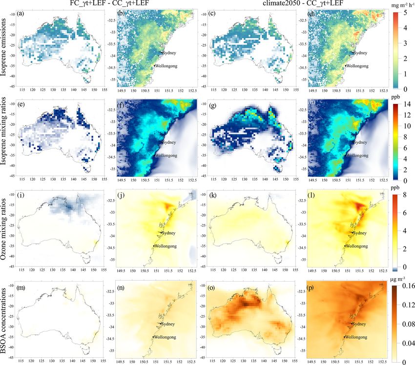
6194                                           K. M. Emmerson et al.: Isoprene emissions from eucalypts in a 2050 climate

1982; Benjamin et al., 1996; Kesselmeier and Staudt, 1999),        mate warming impacts on isoprene emission capacity pro-
emitting isoprene constitutively and storing monoterpenes          vides a lens to study how air quality in Australia could be
within oil reservoirs in the leaves (Brophy et al., 1991). How-    impacted in the future. Using a regional chemical transport
ever, very few of the 800 species in the Eucalyptus genus          model allows us to alter the dynamics of MEGAN to suit
(Department of Agriculture and Water Resources, 2018) have         these new temperature responses for Australia.
been studied for emissions. This is problematic as biogenic           This study aims to (i) determine the temperature response
modellers tend to base simulations on a few measurements           of isoprene in four Eucalyptus species grown under two treat-
which represent a fraction of the potential diversity of species   ments, representing current average summertime tempera-
and emission rates. For example, the Eucalyptus isoprene           tures and a 2050 climate, and (ii) use these measurements
emission factors for the Model of Emissions of Gases and           to determine the impacts of isoprene in a future climate on
Aerosols from Nature (MEGAN) were based on six studies,            predicted levels of O3 and SOA.
only one of which was conducted in Australia (see Emmer-
son et al., 2016). The Australian study measured large differ-
ences of 63 µg g−1 h−1 of isoprene between the lowest- and         2     Methods
highest-emitting eucalypt species, with E. globulus showing
the greatest emission rates (He et al., 2000). Natural occur-      2.1    The MEGAN default temperature response
rence of E. globulus is restricted to temperate south-east Aus-
                                                                   Guenther et al. (2012) define the emission of BVOCs in terms
tralia (including Tasmania).
                                                                   of activity factors representing the environmental conditions
   Use of landscape emission factors (LEFs) weighted by
                                                                   described above. Here we are interested in studying the tem-
higher-emitting trees has caused over-predictions in mod-
                                                                   perature response of isoprene, γ T (unitless):
elled isoprene (Emmerson et al., 2016, 2019a). As young
leaves tend to emit more isoprene than older leaves, conduct-
                                                                                            CT 2 × exp(CT 1 × x)

ing emission measurements on saplings has been questioned           γ T = Eopt ×                                           , (1)
                                                                                     (CT 2 − CT 1 × (1 − exp(CT 2 × x)))
(Street et al., 1997), although adult trees will contain a mix-
ture of leaf ages. However, BVOC emission models such as           where Eopt is the optimum emission point, and CT 1
MEGAN require isoprene emission rates to be determined at          (95 kJ mol−1 ) and CT 2 (230 kJ mol−1 ) are coefficients that
standard conditions of 303 K and 1000 µmol m−2 s−1 photo-          fit the response to a range of ecosystems.
synthetically active radiation (PAR) (Guenther et al., 2012).
Measurements made at other temperatures and PAR fluxes                      (1/Topt ) − (1/T )
                                                                    x=                           ,                           (2)
need scaling to these standard conditions, which can intro-                     0.00831
duce uncertainties of up to 20 % (He et al., 2000). The stan-
dard temperature and light level conditions are better pro-        where T is the temperature of the leaf (K) and 0.00831 is the
vided for in a controlled greenhouse environment, which ne-        gas constant (kJ K−1 mol−1 ). The optimum temperature for
cessitates using saplings.                                         emission throughout MEGAN, Topt , is calculated below.
   MEGAN describes the emission of BVOCs in terms of
temperature, PAR, leaf area index, leaf age, soil moisture         Topt = Tmax + (0.6 × (T240 − TS ))                          (3)
and suppression via ambient CO2 concentrations. Whilst the         Eopt = Ceo × exp(0.05 × (T24 − TS ))
MEGAN parameterisations are fitted from a wide range of                  × exp(0.05 × (T240 − TS )),                           (4)
ecosystem responses to environmental conditions, there are
spatial and temporal exceptions to these standards, which are      where Tmax is 313 K, TS is the standard leaf temperature
comprehensively reviewed by Niinemets et al. (2010). Many          (297 K), and T24 and T240 are the average leaf temperatures
studies have investigated impacts of climate change on iso-        of the previous 24 and 240 h, respectively. Ceo is an empirical
prene by changing the inputs to MEGAN, such as ambient             coefficient of 2 for isoprene.
temperatures and CO2 concentrations (e.g. Bauwens et al.,
2018), and have also investigated how land use might change        2.2    Experimental conditions
the geographical extent of plant functional types (PFTs)
(e.g. Arneth et al., 2011) without changing the MEGAN pa-          Four eucalypt species were chosen based on their prevalence
rameterisations themselves. Here we report new controlled          in Australia and in particular New South Wales (Table 1).
isoprene response measurements from four eucalypt tree             E. camaldulensis and E. tereticornis have a wide geograph-
species, which show different temperature responses than as-       ical representation within Australia, with a latitudinal native
sumed by MEGAN. We also use the controlled experimen-              growing range of 9–38◦ S (Atlas of Living Australia, 2019)
tal conditions to impose a projected 2050 climate to investi-      (Supplement Fig. S1). E. camaldulensis is the most widely
gate whether eucalypts growing in a warmer climate show a          naturally distributed species of all eucalypts in Australia (At-
different temperature sensitivity of isoprene emissions than       las of Living Australia, 2019). The native climatic distribu-
eucalypts growing in the current climate. Accounting for cli-      tion range of E. botryoides and E. smithii is restricted to the

Atmos. Chem. Phys., 20, 6193–6206, 2020                                              https://doi.org/10.5194/acp-20-6193-2020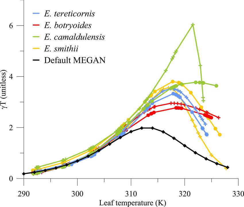
K. M. Emmerson et al.: Isoprene emissions from eucalypts in a 2050 climate                                                                                                     6195

Table 1. Geographic range size of each Eucalyptus species in Australia and the isoprene emission rate based on dry leaf weight.

        Tree                      Common name                      Area (km2 )a         % weight         Emission category           Average emission (µg g−1 h−1 )
        E. camaldulensis          River red gum                       6 040 600              86.32       high                               16.6b 28.0c 32.5d
        E. tereticornis           Forest red gum                        792 575              11.32       high                                   32.7e 38.2f
        E. smithii                Blackbutt peppermint                   95 750               1.37       unknown                                     –
        E. botryoides             Bangalay                               74 175               1.06       moderate                                   5.3b
      a Species area in 2014 (from González-Orozco et al., 2016). b He et al. (2000). c Karkik and Winer (2001). d Benjamin et al. (1996). e Nelson et al. (2000). f Jiang et al.
      (2020), from trees growing in ambient CO2 concentrations.

south-east coastal regions. All four species are forecast to ex-                               flow rate through the cuvette was set to 700 µmol s−1 . Light
ist in future, but only E. camaldulensis is predicted to expand                                was provided using LumiGrow Pro 325 LED growth lamps
its growing area by 2085 (González-Orozco et al., 2016).                                       (LumiGrow, Novato, CA, USA) positioned above the cuvette
   Plant species can be classified as low (less than                                           to provide 1000 µmol m−2 s−1 PAR as measured by the LI-
1 µg g−1 h−1 ), moderate (1–10 µg g−1 h−1 ) or high (greater                                   6400XT cuvette’s light sensor. Leaf temperature was con-
than 10 µg g−1 h−1 ) isoprene emitters (Benjamin et al.,                                       trolled using the Walz cuvette and was programmed to in-
1996). Of the four eucalypts used in this study, E. camal-                                     crease leaf temperature in 5 K steps from 293 to 328 K in
dulensis and E. tereticornis are high isoprene emitters (Ta-                                   7 min intervals to accommodate adjustment to new steady-
ble 1), whilst E. botryoides is classed as moderate. The emis-                                 state values of photosynthesis at each temperature. This time
sion category of E. smithii is unknown. All tabulated mea-                                     corresponds to the duration of intermediate-length sunflecks
surements were scaled to the standard conditions from other                                    in plant canopies (Pearcy, 1990) and also results in a com-
temperatures and PAR.                                                                          mon, standardised heat dose for all the leaves (Niinemets and
   Eighty trees (20 of each species) were grown from seed                                      Sun, 2015). Basal emission rates are taken as the emission
at Hawkesbury Institute for the Environment in Richmond,                                       rate measured at 1000 µmol m−2 s−1 PAR and 303 K.
NSW. After 8 weeks seedlings were transplanted into 6.9 L                                         After the gas exchange measurements, leaves were de-
pots filled with alluvial soil and split randomly into two treat-                              tached and their area measured using an LI-3100C leaf area
ment groups, each containing 10 seedlings of each species.                                     meter (LI-COR, Inc.). Leaves were oven-dried at 105 ◦ C for
The first treatment group was grown for 85 d at an average                                     72 h, after which their dry weight was recorded.
daily temperature of 291 K (current climate), and the sec-                                        Mixing ratios of isoprene by volume were determined
ond treatment group was grown for 85 d at 294.5 K (future                                      using a high-resolution proton-transfer-reaction mass spec-
climate). In this time the seedlings put on vigorous growth                                    trometer (PTR-MS, Ionicon GmbH, Innsbruck, Austria). The
and developed into ∼ 1.5 m tall saplings with plenty of leaves                                 operating parameters of the PTR-MS were held constant dur-
(see Supplement Fig. S2). The future-climate treatment rep-                                    ing measurements except for the secondary electron mul-
resents temperature conditions in Australia in 2050 assuming                                   tiplier voltage, which was optimised before every calibra-
RCP8.5, the highest Representative Concentration Pathway                                       tion. The drift tube pressure, temperature and voltage were
(RCP), in which the business-as-usual scenario sees CO2                                        2.2 hPa, 50 ◦ C and 600 V, respectively. The parameter E/N
reach 940 ppm by 2100 (van Vuuren et al., 2011). The treat-                                    was ∼ 125 Td (1.25 × 10⁻¹⁵ V cm2 ) and the reaction time
ments maintained the diurnal variation of the ambient tem-                                     was ∼ 100 µs. The count rate of H3 O+ qH2 O ions was 1 %–
perature at 9 K. Further details on the growth conditions of                                   2 % of the count rate of H3 O+ ions, which was 5.0–5.5 ×
these eucalypts are described in Aspinwall et al. (2019) prior                                 106 s−1 . Normalised sensitivities and isoprene volume mix-
to their study of how eucalypts respond to heatwave stress.                                    ing ratios were calculated through calibrations as described
   We will use our new experimental data to revise the LEF                                     by Taipale et al. (2008) using 5 ppmv isoprene (Apel-Riemer
maps for Australia, weighting the results according to the                                     Environmental Inc., Broomfield, CO, USA) diluted in high-
summed area of the four species (Table 1).                                                     purity nitrogen (BOC Ltd, Sydney, NSW, Australia). Proto-
                                                                                               nated isoprene was detected by the PTR-MS as its molecular
2.3     Temperature response measurements                                                      mass plus 1 (i.e. M + H + 1 = 69). The duty cycle for each
                                                                                               measurement period was 5 s.
Leaf gas exchange measurements were made continuously                                             Isoprene–temperature response measurements were repli-
with an LI-6400XT portable photosynthesis system (LI-                                          cated on five or six saplings of each species in each tem-
COR, Inc., Lincoln, NE, USA) connected to a Walz 3010-                                         perature treatment group (Supplement Fig. S3). The Solver
GWK1 leaf cuvette (maximum leaf surface area of 140 cm2 ;                                      program (generalised reduced gradient non-linear method,
Heinz Walz GmbH, Effeltrich, Germany). The Walz cuvette                                        default settings; Microsoft Excel for Office 365; Microsoft
was controlled via a PC using Walz software (GFS-Win                                           Corporation, Redmond, WA, USA) was used to estimate four
v.3.47g). CO2 concentrations were set to 400 ppmv, and the

https://doi.org/10.5194/acp-20-6193-2020                                                                              Atmos. Chem. Phys., 20, 6193–6206, 2020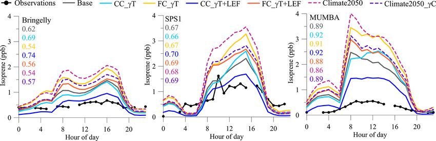
6196 K. M. Emmerson et al.: Isoprene emissions from eucalypts in a 2050 climate
dition to BVOCs, the framework has successfully predicted
pollen (Emmerson et al., 2019b), health effects from ship-
ping (Broome et al., 2016) and air quality (Chambers et al.,
2019). The C-CTM is driven by meteorology from the Con-
formal Cubic Atmospheric Model (CCAM; McGregor and
Dix (2008)), taking boundary conditions from ERA-Interim.
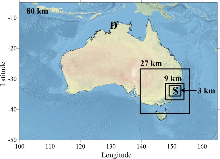
Four nested domains are used at spatial resolutions of 80,
27, 9 and 3 km to downscale the atmospheric constituents
over topography that increases with complexity at higher
resolutions. The inner 3 km domain contains 114 × 110 grid
cells to encompass Sydney, Wollongong and the surrounding
forested regions (Fig. 1).
The model chemistry scheme is MOZART-T1 (Emmons
et al., 2020), incorporating the latest research on isoprene
oxidation pathways via additional radical production under
low-NOx conditions. The aerosol framework is a two-bin
Figure 1. Map to show nests of model domains from 80 km
Australia-wide to 3 km inner Sydney domain. “S” and “D” mark
sectional scheme, processing organic species by the volatility
the locations of Sydney and Darwin, respectively. basis set (Shrivastava et al., 2008) and processing inorganic
species via ISORROPIA_II (Fountoukis and Nenes, 2007).
The high- and low-NOx aerosol mass yields for the organic
MEGAN coefficients, CT 1 , CT 2 , Tmax and Ceo , to minimise species, including isoprene, are provided by Tsimpidi et al.
the difference between the result of Eq. (1) and the measured (2010).
temperature responses for each tree species and growth tem- Australia-wide anthropogenic emissions come from an in-
perature treatment. The basal emission rates for each species ventory based on human population density on a 10 km ×
(µg g−1 h−1 ) were normalised to the average basal emission 10 km grid resolution (updated from Physick et al., 2002).
factor for that species and its growth temperature treatment. Anthropogenic emissions for Sydney in the 3 km domain are
Normalising these data scales the actual emission rates and based on the most recent NSW inventory for the year 2008
ensures they have a common basal emission factor of unity. (EPA NSW, 2012). The full-canopy-environment version of
MEGAN, version 2.1 (Guenther et al., 2012), was built into
2.4 Observations of isoprene mixing ratios the C-CTM to calculate the biogenic emissions (Emmerson
et al., 2016). Isoprene emissions, R, in a given grid cell, xy,
Few measurements of ambient isoprene exist in Australia. are predicted using LEF maps in combination with the land
Hourly observations made by proton-transfer-reaction mass fraction, χ, occupied by 16 PFTs, j , using
spectrometry are available for three summertime urban field
nPFT
campaigns near Sydney (Fig. 1). These observations will be R = LEFx,y
X
(γx,y × χj ), (5)
used to evaluate model predictions using our temperature j =1
response functions of isoprene emission. Isoprene observa-
tions are available from Bringelly for January and Febru- where γ represents the sum of all activity factors for light,
ary of 2007, from SPS1 in Westmead for February and temperature, soil moisture, leaf area index and leaf age. The
March of 2011 (Keywood et al., 2019), and from MUMBA γ for soil moisture is applied using data provided by the Soil–
in Wollongong for January and February of 2013 (Paton- Litter–Iso model (SLI), as recommended by Emmerson et al.
Walsh et al., 2017, 2018). Maximum (and average) measured (2019a). Monthly leaf area index data come from MODIS
temperatures were 308.9 K (295.9 K) for Bringelly, 310.0 K MCD15A2 version 4.
(295.6 K) for SPS1 and 317.2 K (295.3 K) for MUMBA. Cli- A PFT map based on the ESA CCI Land Cover distribution
mate projections for Australia forecast increases in aver- for the year 2010 (ESA, 2016) was created. The ESA land
age temperatures with an accompanying increase in the fre- cover data were used in conjunction with the MODIS 44B
quency of extreme heatwave days (Bureau of Meteorology (Vegetation Continuous Fields) product level 5.1 for the year
and CSIRO, 2018). 2012 to provide the percentage of tree, grass and shrub cover.
Details on how these land cover data were aggregated or split
2.5 The CSIRO Chemical Transport Model into the 16 PFTs required by MEGAN2.1 are provided in
the Supplement. Eucalypts fall under the broadleaf evergreen
The CSIRO Chemical Transport Model (C-CTM) is a mod- temperate tree category.
elling framework designed to predict the atmospheric con-
centrations of gases and aerosols due to emissions, trans-
port, chemical production and loss, and deposition. In ad-
Atmos. Chem. Phys., 20, 6193–6206, 2020 https://doi.org/10.5194/acp-20-6193-2020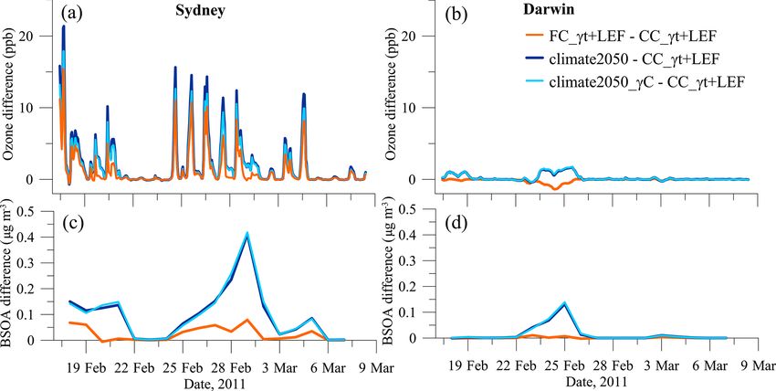
K. M. Emmerson et al.: Isoprene emissions from eucalypts in a 2050 climate                                                      6197

                                                                       for E. tereticornis and E. smithii, decreasing at higher leaf
                                                                       temperatures. Both E. camaldulensis and E. botryoides per-
                                                                       sist at high γ T until 328 K, when measurements stopped. For
                                                                       trees grown under future-climate conditions, the γ T peak is
                                                                       also ∼ 317 K, and there is a different response of E. camaldu-
                                                                       lensis and E. botryoides compared to the other species. γ T in
                                                                       E. camaldulensis increases steeply with increasing leaf tem-
                                                                       perature until 321.5 K, thereafter decreasing sharply. This re-
                                                                       sponse is common amongst the five E. camaldulensis in the
                                                                       future-climate treatment, although there is scatter around this
                                                                       fitted response. The E. camaldulensis result will dominate the
                                                                       weighted variables used in the modelling because of its larger
                                                                       geographic distribution (Table 1). We discuss the impact of
                                                                       this sharp downturn in γ T at high temperatures in Sect. 3.3.

                                                                       3.2   Isoprene emission rates

                                                                       The basal isoprene emission rates (BERs; µg g−1 h−1 ) were
Figure 2. Comparison of γ T with leaf temperature calculated us-       measured at the standard 303 K and 1000 µmol m−2 s−1 PAR
ing default values in MEGAN to results from four eucalypt tree
                                                                       (Table 2). As the current-climate growth treatment repre-
species under current-climate (filled circles) and future-climate (+
                                                                       sents present-day climatic conditions, we only compare these
sign) growth conditions.
                                                                       with measurements made previously on the same species.
                                                                       The E. tereticornis BER measurements are lower than those
                                                                       made by Nelson et al. (2000) and Jiang et al. (2020); how-
3     Results and discussion                                           ever our E. camaldulensis BER measurements are around
                                                                       10 µg g−1 h−1 higher than those listed by Benjamin et al.
3.1    Temperature response results                                    (1996), and our E. botryoides BER measurements are ∼
                                                                       37 µg g−1 h−1 higher than those measured by He et al. (2000).
The fitted temperature responses for each eucalypt tree
                                                                       He et al. (2000) used a mixture of young and mature leaves
species under both current- and future-climate growth con-
                                                                       in their experiments, which could be one explanation for
ditions are stronger and shifted to higher leaf temperatures
                                                                       the difference in emission rates as young leaves are ex-
than the MEGAN2.1 default response (Fig. 2). The peaks
                                                                       pected to be higher emitters than older leaves in Eucalyp-
in current-climate γ T are 40 %–90 % higher than the de-
                                                                       tus species (Street et al., 1997). However, as the growth
fault MEGAN, whilst the peaks in future-climate γ T are
                                                                       conditions (particularly light and temperature) and measure-
45 %–200 % higher. The position of the peaks is also shifted
                                                                       ment protocols in this study and He et al. (2000) were dif-
towards higher temperature optimums by approximately 4–
                                                                       ferent (we directly measured BER with a leaf cuvette at
9 K. For the current-climate growth treatment results, run-
                                                                       303 K and 1000 µmol m−2 s−1 PAR, while He et al., 2000,
ning MEGAN with default settings would underestimate γ T
                                                                       used a dynamic chamber and scaled emissions to 303 K
and subsequently the isoprene emission at leaf temperatures
                                                                       and 1000 µmol m−2 s−1 PAR using algorithms from Guen-
greater than 303 K. MEGAN assumes that at growth tem-
                                                                       ther et al., 1993), it is difficult to undertake a direct com-
peratures lower than the standard conditions, the amplitude
                                                                       parison. However, our measurements put the four eucalypt
of the temperature response (Eopt ) is lowered, and the peak
                                                                       species into the high-emission category.
of that response is shifted to a lower temperature (Topt ).
                                                                          To create new isoprene emission factor maps suitable for
These new data show that this is not necessarily true for all
                                                                       the modelling, we convert the BERs into landscape emission
species studied at each growth temperature. Our measure-
                                                                       factors (LEFisop ). The average BER for each growth treat-
ments also indicate that eucalypts have evolved to cope with
                                                                       ment is weighted according to its respective geographical
the high Australian temperatures and can continue to protect
                                                                       area in Table 1. BERs are then converted into LEFs using
themselves against heat damage via isoprene emission until
                                                                       the leaf mass per unit area (LMA) in grams per square metre
∼ 320 K. Tree species with wide geographical coverage such
                                                                       and scaled with the leaf area index (LAI) in square metres
as E. camaldulensis may also be better adapted to surviving
                                                                       per square metre, similar to Emmerson et al. (2018). The iso-
climate change (González-Orozco et al., 2016).
                                                                       prene emission factor for trees in each temperature treatment
   Each tree in each temperature treatment group produces a
                                                                       is given by tree_EFisop :
similar response (number of trees and their temperatures at
maximum γ T given in Table 2). For trees grown in the cur-
rent climate, the temperature optimum in γ T is 317–318 K              tree_EFisop = BER × LAI × LMA.                             (6)

https://doi.org/10.5194/acp-20-6193-2020                                                Atmos. Chem. Phys., 20, 6193–6206, 2020
6198 K. M. Emmerson et al.: Isoprene emissions from eucalypts in a 2050 climate
Table 2. Average isoprene basal emission rates (BER), leaf mass per unit area (LMA) and temperature at maximum γ T from each pool of
trees under the current- and future-climate growth conditions. Values in brackets are standard deviations. Data in the right-hand column are
derived from model fits.
Treatment Species No. of trees BER, µg g−1 h−1 LMA, g m−2 Temp at max γ T , K
Current climate E. tereticornis 6 29.14 (13.91) 61.53 (5.42) 317.8
E. smithii 6 41.21 (17.31) 54.93 (13.71) 317.8
E. botryoides 6 42.46 (23.64) 72.51 (15.25) 318.4
E. camaldulensis 6 42.87 (22.87) 72.79 (6.14) 322.1
Future climate E. tereticornis 6 41.57 (28.08) 64.05 (9.58) 317.3
E. botryoides 5 55.18 (27.27) 77.96 (12.55) 317.5
E. smithii 6 61.61 (20.01) 58.08 (5.10) 317.0
E. camaldulensis 5 66.95 (22.44) 73.18 (4.64) 321.5
In the C-CTM, northern Australian vegetation is represented CT 1 variable has the least and Ceo has the most impact on
by broadleaf shrubs (30 %–40 %) and C4 grasses (50 % to isoprene emissions. The high CT 2 value in the future-climate
80 % in some locations). If the isoprene emission factor maps treatment will not be refitted as the incurred 19 % decrease in
are only based on the new eucalypt BERs, these are unlikely isoprene is small compared with the 282 % increase caused
to be representative of shrubs and grasses. Here we ensure the by Ceo . Individually, Ceo has the greatest impact on isoprene
non-tree fraction of grid cells in Australia is not impacted by emissions but is regulated by increasing Tmax when used in
these changes using the tree fraction (treefrac) from the ESA tandem with other variables. However, when all variables op-
product. erate together the overall impact is an ∼ 80 % increase in iso-
prene emissions for both current- and future-climate growth
LEFisop = (tree_EFisop × treefrac) conditions. Inclusion of the average LEF reduces the maxi-
+ (orig_EFisop × (1 − treefrac)) (7) mum isoprene emission by 7 % in the current-climate treat-
ment conditions and increases by 23 % in the future-climate
This leaves the fraction of original isoprene LEFs treatment conditions on the default.
(orig_EFisop ) untouched for grass and shrub PFTs.
3.4 Model experiment set-up
3.3 Impacts of changing CT 1 , CT 2 , Tmax and Ceo
Seven model experiments are defined (Table 4) and are run
Table 3 shows the results of fitting CT1 , CT2 , Tmax and Ceo for the periods of the field campaigns described in Sect. 2.4.
compared to the default MEGAN values. These new fitted We model the impacts of using the new current- and future-
data are for the four tree species in the experiment, weighted climate treatment temperature response variables separately
according to their coverage in Table 1. The new average from the impacts of the new LEFs on atmospheric isoprene
LEFs from our four eucalypt species are 31 %–48 % lower mixing ratios. For experiments 1 to 5, we use the same
than the default average MEGAN LEF we use in the base hourly meteorology, present-day tree distribution maps and
run for the 3 km Sydney domain. Previous modelling showed LAI datasets to drive the C-CTM. This allows us to sepa-
that a 40 % reduction in isoprene was needed to better match rate the temperature effect in isoprene emissions from other
the observations from our three field campaigns (Emmerson influences which may change in a future climate. The inten-
et al., 2019a). tion is to investigate changes in isoprene emissions resulting
The value fitted for CT 2 is very high (1158.36 kJ mol−1 ) from the temperature response results, not to combine these
in the future-climate treatment compared with the current- with future land use changes and how the hourly meteorology
climate treatment (167.11 kJ mol−1 ) and default MEGAN will be impacted by climate change. However, in experiment
(230 kJ mol−1 ) due to the E. camaldulensis measurements 6 we use a simple delta-scaling approach to address how a
in Fig. 2. To assess whether CT 2 should be re-fitted we ex- future climate may impact the driving input temperatures to
amine the impacts of changing each of these variables one MEGAN.
at a time using a MEGAN box model designed in Jiang We take the average change (δ2050) in projected summer-
et al. (2020). As the impacts of the new measurements are time surface temperatures for Australia under the RCP8.5
strongest at higher temperatures, we assume conditions from scenario from eight models in the Coupled Model Inter-
the hottest day in the MUMBA campaign (18 January 2013). comparison Project 5 (CMIP5) (for details see Supplement).
The MEGAN box model runs for 24 h, and the results are Delta-scaling adds ∼ 2 K to the surface temperatures near
given as percentage changes to the maximum isoprene emis- Sydney. We only scale the surface temperature; thus experi-
sion in Table 3. For the given fitted values on this day, the ment 6 is not a 2050 representation of the whole atmosphere.
Atmos. Chem. Phys., 20, 6193–6206, 2020 https://doi.org/10.5194/acp-20-6193-2020K. M. Emmerson et al.: Isoprene emissions from eucalypts in a 2050 climate 6199
Table 3. Changes to MEGAN variables based on fitted data from current- and future-climate growth experiments. Percentages in brackets
indicate change in maximum daily isoprene emissions due to change in variable.
MEGAN2.1 Current-climate Future-climate
growth treatment growth treatment
Average LEF (µg g−1 h−1 ) 9491∗ 4919 (−48 %) 6585 (−31 %)
CT 1 (kJ mol−1 ) 95 110.55 (−1 %) 75.04 (+1 %)
CT 2 (kJ mol−1 ) 230 167.11 (+5 %) 1158.36 (−19 %)
Tmax (K) 313 325 (−55 %) 323 (−46 %)
Ceo 2 6.77 (+238 %) 7.69 (+282 %)
All variables without LEF +81 % +76 %
All variables + LEF −7 % +23 %
∗ Value of average LEF from the inner 3 km domain.
Table 4. Description of each model experiment. CC: current climate; FC: future climate.
Experiment Name Emission Temperature Meteorology used to γC
factors response drive MEGAN
1 Base default default current x
2 CC_γ T default fitted CC current x
3 CC_γ T +LEF CC LEF fitted CC current x
4 FC_γ T default fitted FC current x
5 FC_γ T +LEF FC LEF fitted FC current x
6 Climate2050 FC LEF fitted FC current + δ2050 x
7 Climate2050_γ C FC LEF fitted FC current + δ2050 X
This restricts the use of the delta-scaled temperatures as a in isoprene emission in the FC_γ T and FC_γ T +LEF exper-
MEGAN input and not the temperature used for chemical re- iments after 324 K is due to the high γ T of E. camaldulen-
actions as mass balance difficulties would occur by not also sis depicted in Fig. 2. However, these results will not impact
delta-scaling the pressure and air density through the height the C-CTM runs as no hourly temperature in our three field
of the atmosphere. We estimate that the reaction rate of iso- campaigns exceeds 317 K. Most of the impacts on the C-
prene with OH (calculated as 2.54 × 10⁻¹¹ exp(410/T ) in CTM runs will occur in the 288–308 K range. While there is
MOZART-T1) would decrease by 1.7 % with the 3.5 K tem- a very small decrease in the CC_γ T response compared with
perature rise between our current- and future-climate growth the default MEGAN profile at temperatures less than 300 K,
treatments. overall we expect more isoprene to be emitted in the CC_γ T
The climate2050 run does not include the associated in- and FC_γ T experiments than in the default MEGAN profile.
creases in CO2 mixing ratios, to be consistent with our mea- While it is intuitive to expect less isoprene to be emitted in
surements that were also not conducted in a higher-CO2 at- the CC_γ T +LEF and FC_γ T +LEF experiments than in the
mosphere. A seventh simulation assumes a 550 ppm CO2 at- base run (from Fig. 3), this may not be the case due to spa-
mosphere on top of the delta-scaled surface temperatures, tial heterogeneity in the new current- and future-climate LEF
employing the Heald et al. (2009) method for calculating maps. The LEFs used in Fig. 3 are based on the domain spa-
short- and long-term CO2 activity factors, γ C. Fixing the at- tial average value; however the LEFs in experiments 3 and
mospheric CO2 to 550 ppm reduces the isoprene emissions 5 are based on the distribution of LAI from Eq. (6), whilst
by 5 % in the short term and 13 % in the long term. experiments 1, 2 and 4 use the original MEGAN LEF distri-
If the leaf temperature is varied within Eqs. (1)–(4) and bution. The results from experiments 3 and 5 certainly show
γ T is multiplied by the LEF, the impacts of experiments 1– a sustained isoprene decrease below 314 and 311 K, respec-
5 on isoprene emission start at about 283 K (Fig. 3). Ex- tively. Distance from source to receptor, transport and dilu-
periment 6 follows the FC_γ T +LEF profile. Here, the new tion will all impact results and are determined by running the
current- and future-climate LEFs are normalised by the de- C-CTM.
fault MEGAN LEF. The default MEGAN profile has a peak
isoprene emission at 311 K. The CC_γ T and FC_γ T exper-
iments cause the isoprene emission peak to shift to 324 K,
with 3 times the default emission value. The sharp downturn
https://doi.org/10.5194/acp-20-6193-2020 Atmos. Chem. Phys., 20, 6193–6206, 20206200 K. M. Emmerson et al.: Isoprene emissions from eucalypts in a 2050 climate
stresses (Loreto and Fineschi, 2015) above and beyond leaf
cooling via transpiration processes (Sharkey et al., 2008).
High isoprene emitters can better survive prolonged heat-
waves (Yáñez-Serrano et al., 2019), although the Aspinwall
et al. (2019) study on our four eucalypt species showed that
trees grown under future-climate conditions suffered greater
heatwave damage than the same species in current-climate
conditions.
During all campaigns the CC_γ T results have decreased
the isoprene from the base runs in the morning between
08:00 and 11:00 AEDT because these temperatures are less
than 303 K, where the γ T values are less than the de-
fault MEGAN profile (Fig. 3). The CC_γ T +LEF experi-
ments represent present-day conditions, with roughly the cor-
rect magnitude (MUMBA excepted) of predicted isoprene
and best statistical fit compared with the observations. The
FC_γ T +LEF experiment has produced more daytime iso-
prene than the base run contrary to the prediction in Fig. 3
because the distribution of isoprene LEFs near the field cam-
Figure 3. Impacts of new MEGAN variables on normalised iso- paign sites is different to the default MEGAN LEFs. The cli-
prene emission rates at increasing ambient temperatures.
mate2050 experiment adds between 110 % and 170 % more
isoprene during the day, or approximately 2 ppb. Across
the three campaigns, the addition of a higher-CO2 atmo-
3.5 C-CTM results sphere reduced the daytime isoprene by 15 %–26 % of the
climate2050 run.
The C-CTM is compiled with changes to MEGAN imple- The MUMBA and SPS1 base diurnal profiles show too
mented according to Table 3, run for experiments 1–6 (Ta- much isoprene in the model overnight compared to observed
ble 4), and the isoprene time series is extracted at each field mean values, particularly in the period between midnight and
campaign site. The modelled mean diurnal profiles of iso- 06:00 AEDT. This is because there is more isoprene in the
prene are then compared to the mean diurnal observations model atmosphere than was quenched by the OH radical be-
taken at each field campaign (Fig. 4). Blank samples are fore the OH production ceased at sundown. The isoprene be-
taken at least twice a day, incurring frequent regular gaps comes more concentrated at the surface because of the re-
in observed isoprene. The CC_γ T variables only increase duced boundary layer height; the apparent increase between
the isoprene mixing ratios when temperatures exceed 303 K midnight and 03:00 AEDT is not due to night-time isoprene
(from Fig. 3). This has changed the shape of the diurnal pro- emissions. Conversely a slight rise in the model boundary
files of each field campaign in different ways, but generally layer at 04:00 AEDT in SPS1 causes dilution of the atmo-
the CC_γ T and CC_γ T +LEF experiments have increased spheric isoprene. While there are few measurements of iso-
the diurnal modelled to observed r 2 when compared with prene during these predawn periods, it is unlikely that iso-
the r 2 between the base run and observations. The average prene is present. Only when daytime isoprene is reduced in
modelled isoprene in the CC_γ T +LEF run is within ±1 the CC_γ T +LEF experiment do we see that the apparent
standard deviation of the observations 90 %–100 % of the night-time isoprene is decreased.
time during Bringelly and SPS1 and 33 % of the time dur- We investigate the spatial changes to isoprene, O3 and
ing MUMBA, which continues to exhibit high bias (Supple- biogenic SOA in an implied future by subtracting results
ment Fig. S4). In MUMBA, the CC_γ T increases the iso- from the CC_γ T +LEF experiment from the climate2050 ex-
prene mixing ratios above the base run between 11:00 and periment during the period of the SPS1 campaign (Fig. 5).
17:00 AEDT in the heat of the day. Very hot temperatures These emissions, mixing ratios and aerosol concentrations
during the day can often be accompanied by strong, gusty represent campaign averages from SPS1. We also show the
winds from the Australian interior. The hottest campaign day smaller differences found between the FC_γ T +LEF and
during MUMBA, 18 January 2013, was associated with the CC_γ T +LEF runs. The climate2050 experiment produces
highest average hourly wind measurement of 8 m s−1 . Hot up to 5.2 mg m−2 h−1 in isoprene emissions to the immediate
and windy conditions would cause lots of sun-flecking within north of Sydney (Fig. 5d), but there are also increases in the
the tree canopy, causing sudden temperature spikes on the north of Australia (Fig. 5c). The largest changes in isoprene,
leaf surface. Physiologically, the increased production of iso- amounting to 15.8 ppb, occur in sparsely inhabited northern
prene during temperature and light spikes helps to maintain Australia (Fig. 5g) and in urbanised pockets to the south and
photosynthesis (Behnke et al., 2010) during times of mild east, where Sydney is located. Urbanisation becomes impor-
Atmos. Chem. Phys., 20, 6193–6206, 2020 https://doi.org/10.5194/acp-20-6193-2020K. M. Emmerson et al.: Isoprene emissions from eucalypts in a 2050 climate 6201
Figure 4. Average diurnal time series in isoprene mixing ratios incurred by the different model experiments at each field campaign site. r 2
values between modelled and observed isoprene given in the same colours as the legend.
tant when the increased isoprene reacts with NOx in the at- large cities will likely encounter more NEPM exceedances.
mosphere, causing a peak increase in O3 of 9 ppb near Syd- The solution is not to remove native trees as they provide
ney with the climate2050 differences (Fig. 5l). However, the social amenity and have cultural significance for indigenous
FC_γ T +LEF differences (Fig. 5i) show a 0.5 ppb decrease populations. Rather, their emissions must be accommodated
in O3 in northern Australia via quenching by the additional via atmospheric NOx reductions. New urban developments
isoprene. Few inhabitants reside in northern Australia, mean- should consider the BVOC emission potential of trees be-
ing O3 production via anthropogenic NOx is minimised. Soil fore planting (Paton-Walsh et al., 2019), taking into account
NOx emissions are low in northern Australia as agricultural that non- or low-emitting trees may not withstand climate-
practices largely occur in the south-east and south-west of induced heatwaves (Peñuelas and Munné-Bosch, 2005).
Australia. The O3 deficit is still visible in the very north-east The SOA from isoprene is a small fraction of the PM2.5
of Australia in the climate2050 difference run (Fig. 5k). The limit (shown here as 24 h averages), though of the BVOC
increase in biogenic SOA occurs mainly in the north of Aus- aerosol yields, isoprene is not expected to dominate. The
tralia, where up to 0.21 µg m−3 more aerosol is predicted by aerosol yields from monoterpenes are 10–20 times higher
the climate2050 experiment than the CC_γ T +LEF experi- than the isoprene yield, and the monoterpene emission would
ment (Fig. 5o). increase in a warming climate (not investigated here). The
The size fraction of most secondary organic aerosol fits climate2050 differences (and climate2050_γ C) show days
within the PM2.5 classification, defined as particulate mat- with an increase of 0.42 µg m−3 in Sydney and 0.14 µg m−3
ter with an aerodynamic diameter less than 2.5 µm. Australia in Darwin (2 % and 1 % of the PM2.5 2025 NEPM, respec-
sets National Environmental Protection Measures (NEPMs) tively).
for PM2.5 and O3 to ensure a healthy standard of air quality
for the population. The NEPM for O3 is 100 ppb as a 1 h aver-
age and 25 µg m−3 as a 24 h average for PM2.5 , with the goal 4 Conclusions
of reducing the PM2.5 limit to 20 µg m−3 by 2025. We exam-
We have measured the isoprene emission response to con-
ine the increases brought about by climate-induced isoprene
trolled increases in temperature from four eucalypt species,
in the two cities impacted most by these changes, Sydney and
two of which have a large geographical growing extent
Darwin, in Australia’s north (Fig. 6).
in Australia. The trees were grown in temperatures repre-
The air quality index (AQI = NEPM/pollutant concentra-
senting current-climate summertime conditions in Australia
tion ×100) in Sydney and Darwin is classed as “very good”
and in temperatures representing the projected summertime
(AQI < 33) for both pollutants (years 2009–2014), with an
conditions of +3.5 K warming under the business-as-usual
improving trend for O3 but a declining trend for PM2.5 (Key-
RCP8.5 scenario. Climate projections for Australia forecast
wood et al., 2016). Darwin is a small city, and the biogenic
increases in average temperatures with an accompanying in-
component of O3 changes is less than 2 ppb. However peak
crease in the frequency of extreme heatwave days (Bureau of
O3 in Sydney increases by 10–15 ppb as an hourly average
Meteorology and CSIRO, 2018). This will likely increase the
in the FC_γ T +LEF differences but by 12–17 ppb in the
number of days above 303 K.
climate2050_γ C differences and by as much as 15–21 ppb
The current-condition experiments demonstrated a change
in the climate2050 differences (Fig. 6a, b). These increases
in the isoprene emission response to temperature as com-
represent 10 %–21 % of the O3 NEPM and show that by do-
pared with the default parameterisation in MEGAN. This
ing nothing (e.g. tree type and coverage or air quality poli-
is not a surprise as MEGAN is built to represent a range
cies do not change) and allowing the temperatures to rise,
in ecosystem responses but may go some way to explain
https://doi.org/10.5194/acp-20-6193-2020 Atmos. Chem. Phys., 20, 6193–6206, 20206202 K. M. Emmerson et al.: Isoprene emissions from eucalypts in a 2050 climate Figure 5. Difference between FC_γ T +LEF and CC_γ T +LEF runs (a, b, e, f, i, j, m, n) during the SPS1 campaign. The difference between the climate2050 runs and CC_γ T +LEF runs is shown in panels (c), (d), (g), (h), (k), (l), (o) and (p). (a–d) Isoprene emission, (e–h) isoprene mixing ratio, (i–l) ozone mixing ratio, (m–p) biogenic SOA concentration in Australia at 80 km and Sydney at 3 km domains. why difficulties have been encountered when modelling iso- weighted emission rates to LEFs for use in the C-CTM re- prene in Australia previously. Both the current- and future- sulted in a lower average LEF than is currently being used climate growth treatment temperature responses shifted the in the base run. This is due to low biomass measured on peak in γ T by 4–9 K, signifying that these four eucalypt our leaves and because the isoprene emission factors from species were observed to continue emitting isoprene until regions described as shrubs or grasslands were not altered. well past the default maximum temperature for emission at The spatial distribution of the new LEFs was based on the 313 K. This suggests that the eucalypts used in this study LAI distribution, which differs from the default MEGAN iso- have evolved to protect themselves against higher tempera- prene LEF map. tures as expected with climate change. The model results using the new current-climate growth Higher basal emission rates were measured in three of the temperature responses improved the statistical fits of the di- eucalypt species in our experiment than have been previ- urnal profiles compared to the measurements of average iso- ously measured. However, the conversion of these average prene across our three field campaign periods. The overall Atmos. Chem. Phys., 20, 6193–6206, 2020 https://doi.org/10.5194/acp-20-6193-2020
K. M. Emmerson et al.: Isoprene emissions from eucalypts in a 2050 climate                                                        6203

Figure 6. Differences in hourly ozone (a, b) and biogenic secondary organic aerosol (c, d) due to three 2050 experiments at Sydney and
Darwin during the SPS1 campaign period.

magnitude of the modelled profile was also brought into bet-         peratures was the simplest way of conducting future-climate
ter agreement with observations in combination with the new          experiments. Future work should investigate getting a down-
current-climate-growth LEFs. MEGAN2.1 essentially works              scaled version of the 2050 atmosphere from the CCAM,
using a series of variables dependent on vegetation type and         which would provide the hourly meteorology throughout the
biogenic compound emission traits, and the results here sug-         atmosphere that the C-CTM requires.
gest that the four MEGAN variables altered in our experi-               The future is expected to bring increased temperatures,
ments could also become ecosystem- or location-specific.             CO2 and land use changes. Sharkey and Monson (2014) eval-
   Our measurements were conducted on sapling trees, which           uated the isoprene trade-off in each of these scenarios and
may exhibit higher isoprene emissions than adult trees when          concluded that the temperature effects would dominate. O3
emission rates are expressed based on leaf mass but not when         is a secondary product of isoprene oxidation and is currently
they are based on leaf area (Street et al., 1997). Street et al.     maintained at healthy levels in Australia. In order to main-
(1997) attributed this to younger leaves having a higher spe-        tain these levels, air quality policy should investigate meth-
cific leaf area than older leaves because eucalypts exhibit het-     ods to reduce anthropogenic NOx emissions in city regions
erophylly (the foliage leaves on the same plant are of two dis-      to accommodate these climate-change-induced increases in
tinctly different types). The apparent difference in emission        BVOC emissions. In addition, tree-planting efforts in new ur-
rates between young and old leaves could be a consequence            ban developments should also consider the BVOC emission
of morphology rather than biochemistry, so we expect the             potential of prospective trees.
trend between the current- and future-climate-growth emis-
sions to be similar amongst trees of all ages. Our model
experiments simulating isoprene emissions in a 2050 cli-             Data availability. The       temperature     response       mea-
mate examined the differences between these runs and the             surements reported in this paper are available from
CC_γ T +LEF experiment. Three future experiments were                https://doi.org/10.25919/5ea918835c3fc (Emmerson et al.,
conducted, the first using present-day meteorology, the sec-         2020) along with modelled time series data used in Figs. 4 and 6.
                                                                     The LAI data product was retrieved from MCD15A2 version 4
ond using a delta-scaled surface temperature change to pro-
                                                                     from the online Data Pool, courtesy of the NASA Land Processes
jected 2050 summertime temperatures and the third using a            Distributed Active Archive Center (LP DAAC), USGS/Earth
550 ppm atmospheric CO2 on top of the delta-scaled temper-           Resources Observation and Science (EROS) Center, Sioux Falls,
atures. The FC_γ T +LEF experiment showed increases in               South Dakota, https://lpdaac.usgs.gov/data_access/data_pool (last
isoprene emissions in the north of Australia as well as closer       access: June 2004; NASA LP DAAC, 2004).
to Sydney. These increases led to O3 rising 10–15 ppb close
to Sydney as a result of the increased isoprene whilst decreas-
ing in sparsely populated northern Australia through quench-         Supplement. The supplement related to this article is available on-
ing by the additional isoprene. The climate2050 experiment           line at: https://doi.org/10.5194/acp-20-6193-2020-supplement.
showed much larger increases in isoprene, O3 and biogenic
SOA across Australia, tempered slightly by the addition of
increased atmospheric CO2 . Delta-scaling the surface tem-

https://doi.org/10.5194/acp-20-6193-2020                                               Atmos. Chem. Phys., 20, 6193–6206, 2020
6204 K. M. Emmerson et al.: Isoprene emissions from eucalypts in a 2050 climate
Author contributions. KME and MP devised the modelling study Brophy, J. J., House, A. P. N., Boland, D. J., and Lassak, E. V.: Di-
and wrote the manuscript. KME conducted the modelling. MP, gest of the essential oils of 111 species from northern and eastern
MJA, SP and MGT conducted the experimental work. MJA, SP and Australia, in: Eucalyptus Leaf Oils: Use, Chemistry, Distillation
MGT edited the manuscript. and Marketing, edited by: Boland, D. J., Brophy, J. J., and House,
A. P. N., Inkarta Press, Melbourne, 129–155, 1991.
Bureau of Meteorology and CSIRO: State of the Climate 2018,
Competing interests. The authors declare that they have no conflict available at: http://www.bom.gov.au/state-of-the-climate/index.
of interest. shtml (last access: 18 October 2019), 2018.
Chambers, S. D., Guerette, E.-A., Monk, K., Griffiths, A. D., Zhang,
Y., Duc, H., Cope, M., Emmerson, K. M., Chang, L. T., Silver,
Acknowledgements. Kathryn M. Emmerson thanks Christine J. D., Utembe, S., Crawford, J., Williams, A. G., and Keywood,
Wiedinmyer at the University of Colorado Boulder for assistance M.: Skill-Testing Chemical Transport Models across Contrasting
with the ESA land cover product data and John Clarke at CSIRO Atmospheric Mixing States Using Radon-222, Atmosphere, 10,
for helpful discussions on using the climate projection data. 25, https://doi.org/10.3390/atmos10010025 2019.
Department of Agriculture and Water Resources: Australia’s State
of the Forests Report 2018, available at: https://www.agriculture.
gov.au/abares/forestsaustralia/sofr/sofr-2018 (last access: 2 De-
Review statement. This paper was edited by Janne Rinne and re-
cember 2019), 2018.
viewed by two anonymous referees.
Emmerson, K. M., Galbally, I. E., Guenther, A. B., Paton-Walsh,
C., Guerette, E.-A., Cope, M. E., Keywood, M. D., Lawson, S.
J., Molloy, S. B., Dunne, E., Thatcher, M., Karl, T., and Malek-
nia, S. D.: Current estimates of biogenic emissions from euca-
References lypts uncertain for southeast Australia, Atmos. Chem. Phys., 16,
6997–7011, https://doi.org/10.5194/acp-16-6997-2016, 2016.
Arneth, A., Schurgers, G., Lathiere, J., Duhl, T., Beerling, D. Emmerson, K. M., Cope, M. E., Galbally, I. E., Lee, S., and Nelson,
J., Hewitt, C. N., Martin, M., and Guenther, A.: Global ter- P. F.: Isoprene and monoterpene emissions in south-east Aus-
restrial isoprene emission models: sensitivity to variability in tralia: comparison of a multi-layer canopy model with MEGAN
climate and vegetation, Atmos. Chem. Phys., 11, 8037–8052, and with atmospheric observations, Atmos. Chem. Phys., 18,
https://doi.org/10.5194/acp-11-8037-2011, 2011. 7539–7556, https://doi.org/10.5194/acp-18-7539-2018, 2018.
Aspinwall, M. J., Pfautsch, S., Tjoelker, M. G., Vårhammar, A., Emmerson, K. M., Palmer, P. I., Thatcher, M., Haverd, V., and
Possell, M., Drake, J. E., Reich, P. B., Tissue, D. T., Atkin, O. K., Guenther, A. B.: Sensitivity of isoprene emissions to drought
Rymer, P. D., Dennison, S., and Van Sluyter, S. C.: Range size over south-eastern Australia: Integrating models and satellite
and growth temperature influence Eucalyptus species responses observations of soil moisture, Atmos. Environ., 209, 112–124,
to an experimental heatwave, Glob. Change Biol., 25, 1665– https://doi.org/10.1016/j.atmosenv.2019.04.038, 2019a.
1684, https://doi.org/10.1111/gcb.14590, 2019. Emmerson, K. M., Silver, J. D., Newbigin, E., Lampugnani, E. R.,
Atlas of Living Australia: Eucalyptus camaldulensis, avail- Suphioglu, C., Wain, A., and Ebert, E.: Development and eval-
able at: https://bie.ala.org.au/species/https://id.biodiversity.org. uation of pollen source methodologies for the Victorian Grass
au/node/apni/2921040, last access: 6 September 2019. Pollen Emissions Module VGPEM1.0, Geosci. Model Dev., 12,
Bauwens, M., Stavrakou, T., Müller, J.-F., Van Schaeybroeck, 2195–2214, https://doi.org/10.5194/gmd-12-2195-2019, 2019b.
B., De Cruz, L., De Troch, R., Giot, O., Hamdi, R., Termo- Emmerson, K. M., Possell, M, Aspinwall, M. J., Pfautsch,
nia, P., Laffineur, Q., Amelynck, C., Schoon, N., Heinesch, S., and Tjoelker, M. G.: Data associated with “Tem-
B., Holst, T., Arneth, A., Ceulemans, R., Sanchez-Lorenzo, perature response measurements from eucalypts give in-
A., and Guenther, A.: Recent past (1979–2014) and future sight into the impact of Australian isoprene emissions
(2070–2099) isoprene fluxes over Europe simulated with the on air quality in 2050”, v1, CSIRO, Data Collection,
MEGAN–MOHYCAN model, Biogeosciences, 15, 3673–3690, https://doi.org/10.25919/5ea918835c3fc, 2020.
https://doi.org/10.5194/bg-15-3673-2018, 2018. Emmons, L. K., Orlando, J. J., Tyndall, G., Schwantes, R. H.,
Behnke, K., Loivamäki, M., Zimmer, I., Rennenberg, H., Schnitzler, Lamarque, J.-F., Marsh, D., Mills, M. J., Tilmes, S., Buch-
J.-P., and Louis, S.: Isoprene emission protects photosynthesis in holz, R. R., Gettelman, A., Garcia, R., Simpson, I., Meinardi,
sunfleck exposed Grey poplar, Photosynthesis research, 104, 5– S., and Pétron, G.: The Chemistry Mechanism in the Commu-
17, https://doi.org/10.1007/s11120-010-9528-x, 2010. nity Earth System Model version 2, J. Adv. Model. Earth Sy.,
Benjamin, M. T., Sudol, M., Bloch, L., and Winer, A. M.: Low- 12, e2019MS001882, https://doi.org/10.1029/2019MS001882,
emitting urban forests: A taxonomic methodology for assign- 2020.
ing isoprene and monoterpene emission rates, Atmos. Environ., EPA NSW: air-emissions-inventory, NSW Environment
30, 1437–1452, https://doi.org/10.1016/1352-2310(95)00439-4, Protection Authority, available at: https://www.epa.nsw.
1996. gov.au/your-environment/air/air-emissions-inventory/
Broome, R. A., Cope, M. E., Goldsworthy, B., Goldsworthy, L., air-emissions-inventory-2008 (last access: 21 May 2020),
Emmerson, K., Jegasothy, E., and Morgan, G. G.: The mortality 2012.
effect of ship-related fine particulate matter in the Sydney greater
metropolitan region of NSW, Australia, Environ. Int., 87, 85–93,
2016.
Atmos. Chem. Phys., 20, 6193–6206, 2020 https://doi.org/10.5194/acp-20-6193-2020K. M. Emmerson et al.: Isoprene emissions from eucalypts in a 2050 climate 6205
ESA: CI Land Cover dataset (v 1.6.1), available at: https://www. Physiology and Ecology, J. Atmos. Chem., 33, 23–88,
esa-landcover-cci.org/?q=node/169 (last access: 4 September https://doi.org/10.1023/A:1006127516791, 1999.
2019), 2016. Keywood, M., Selleck, P., Reisen, F., Cohen, D., Chambers,
Evans, R. C., Tingey, D. T., Gumpertz, M. L., and S., Cheng, M., Cope, M., Crumeyrolle, S., Dunne, E., Em-
Burns, W. F.: Estimates of Isoprene and Monoterpene merson, K., Fedele, R., Galbally, I., Gillett, R., Griffiths, A.,
Emission Rates in Plants, Bot. Gaz., 143, 304–310, Guerette, E.-A., Harnwell, J., Humphries, R., Lawson, S., Mil-
https://doi.org/10.1086/botanicalgazette.143.3.2474826, 1982. jevic, B., Molloy, S., Powell, J., Simmons, J., Ristovski, Z.,
Fountoukis, C. and Nenes, A.: ISORROPIA II: a computa- and Ward, J.: Comprehensive aerosol and gas data set from the
tionally efficient thermodynamic equilibrium model for K+ – Sydney Particle Study, Earth Syst. Sci. Data, 11, 1883–1903,
2−
Ca2+ –Mg2+ –NH+ + − −
4 –Na –SO4 –NO3 –Cl –H2 O aerosols, At- https://doi.org/10.5194/essd-11-1883-2019, 2019.
mos. Chem. Phys., 7, 4639–4659, https://doi.org/10.5194/acp-7- Keywood, M. D., Hibberd, M. H., and Emmerson, K. M.:
4639-2007, 2007. Australia: State of the environment 2016 – Atmosphere,
González-Orozco, C. E., Pollock, L. J., Thornhill, A. H., Mishler, independent report to the Australian Government Minis-
B. D., Knerr, N., Laffan, S. W., Miller, J. T., Rosauer, D. F., Faith, ter for the Environment and Energy, Australian Govern-
D. P., Nipperess, D. A., Kujala, H., Linke, S., Butt, N., Külheim, ment Department of the Environment and Energy, Canberra,
C., Crisp, M. D., and Gruber, B.: Phylogenetic approaches reveal https://doi.org/10.4226/94/58b65c70bc372, 2016.
biodiversity threats under climate change, Nat. Clim. Change, 6, Loreto, F. and Fineschi, S.: Reconciling functions and evolution of
1110–1114, https://doi.org/10.1038/nclimate3126, 2016. isoprene emission in higher plants, New Phytol., 206, 578–582,
Guenther, A. B., Zimmerman, P. R., Harley, P. C., Monson, R. K., https://doi.org/10.1111/nph.13242, 2015.
and Fall, R.: Isoprene and monoterpene emission rate variability: McGregor, J. L. and Dix, M. R.: An updated description of the
Model evaluations and sensitivity analyses, J. Geophys. Res.- Conformal-Cubic Atmospheric Model in High Resolution Sim-
Atmos., 98, 12609–12617, https://doi.org/10.1029/93JD00527, ulation of the Atmosphere and Ocean, edited by: Hamilton, K.
1993. and Ohfuchi, W., 51–76, Springer, 2008.
Guenther, A. B., Jiang, X., Heald, C. L., Sakulyanontvittaya, Millet, D. B., Baasandorj, M., Hu, L., Mitroo, D., Turner,
T., Duhl, T., Emmons, L. K., and Wang, X.: The Model of J., and Williams, B. J.: Nighttime Chemistry and Morn-
Emissions of Gases and Aerosols from Nature version 2.1 ing Isoprene Can Drive Urban Ozone Downwind of a Ma-
(MEGAN2.1): an extended and updated framework for mod- jor Deciduous Forest, Environ. Sci. Technol., 50, 4335–4342,
eling biogenic emissions, Geosci. Model Dev., 5, 1471–1492, https://doi.org/10.1021/acs.est.5b06367, 2016.
https://doi.org/10.5194/gmd-5-1471-2012, 2012. NASA LP DAAC: MODIS leaf area index data product was
He, C., Murray, F., and Lyons, T.: Monoterpene and isoprene emis- retrieved from MCD15A2 version 4 from the online Data
sions from 15 Eucalyptus species in Australia, Atmos. Environ., Pool, courtesy of the NASA Land Processes Distributed Active
34, 645–655, https://doi.org/10.1016/S1352-2310(99)00219-8, Archive Center (LP DAAC), USGS/Earth Resources Observa-
2000. tion and Science (EROS) Center, Sioux Falls, South Dakota,
Heald, C. L., Wilkinson, M. J., Monson, R. K., Alo, C. A., Wang, available at: https://lpdaac.usgs.gov/data_access/data_pool, last
G., and Guenther, A.: Response of isoprene emission to am- access: June 2004.
bient CO2 changes and implications for global budgets, Glob. Nelson, P. F., Nancarrow, P. C., Haliburton, B., Tibbet, A. R., Chase,
Change Biol., 15, 1127–1140, https://doi.org/10.1111/j.1365- D., and Trieu, T.: Biogenic emissions from trees and grasses,
2486.2008.01802.x, 2009. CSIRO investigation Report ET/IR297, Tech. rep., 2000.
Jiang, M., Medlyn, B. E., Drake, J. E., Duursma, R. A., Anderson, Niinemets, Ü. and Sun, Z.: How light, temperature, and
I. C., Barton, C. V. M., Boer, M. M., Carrillo, Y., Castañeda- measurement and growth [CO2 ] interactively control iso-
Gómez, L., Collins, L., Crous, K. Y., De Kauwe, M. G., dos San- prene emission in hybrid aspen, J. Exp. Bot., 66, 841–51,
tos, B. M., Emmerson, K. M., Facey, S. L., Gherlenda, A. N., https://doi.org/10.1093/jxb/eru443, 2015.
Gimeno, T. E., Hasegawa, S., Johnson, S. N., Kännaste, A., Mac- Niinemets, Ü., Arneth, A., Kuhn, U., Monson, R. K., Peñue-
donald, C. A., Mahmud, K., Moore, B. D., Nazaries, L., Neilson, las, J., and Staudt, M.: The emission factor of volatile iso-
E. H. J., Nielsen, U. N., Niinemets, Ü., Noh, N. J., Ochoa-Hueso, prenoids: stress, acclimation, and developmental responses, Bio-
R., Pathare, V. S., Pendall, E., Pihlblad, J., Piñeiro, J., Powell, geosciences, 7, 2203–2223, https://doi.org/10.5194/bg-7-2203-
J. R., Power, S. A., Reich, P. B., Renchon, A. A., Riegler, M., 2010, 2010.
Rinnan, R., Rymer, P. D., Salomón, R. L., Singh, B. K., Smith, Paton-Walsh, C., Guérette, É.-A., Kubistin, D., Humphries, R.,
B., Tjoelker, M. G., Walker, J. K. M., Wujeska-Klause, A., Yang, Wilson, S. R., Dominick, D., Galbally, I., Buchholz, R., Bhu-
J., Zaehle, S., and Ellsworth, D. S.: The fate of carbon in a mature jel, M., Chambers, S., Cheng, M., Cope, M., Davy, P., Emmer-
forest under carbon dioxide enrichment, Nature, 580, 227–231, son, K., Griffith, D. W. T., Griffiths, A., Keywood, M., Law-
https://doi.org/10.1038/s41586-020-2128-9, 2020. son, S., Molloy, S., Rea, G., Selleck, P., Shi, X., Simmons, J.,
Karkik, J. and Winer, A.: Measured isoprene emission rates and Velazco, V.: The MUMBA campaign: measurements of ur-
of plants in California landscapes: comparison to estimates ban, marine and biogenic air, Earth Syst. Sci. Data, 9, 349–362,
from taxonomic relationships, Atmos. Environ., 35, 1123–1131, https://doi.org/10.5194/essd-9-349-2017, 2017.
https://doi.org/10.1016/S1352-2310(00)00258-2, 2001. Paton-Walsh, C., Guérette, E.-A., Emmerson, K., Cope,
Kesselmeier, J. and Staudt, M.: Biogenic Volatile Or- M., Kubistin, D., Humphries, R., Wilson, S., Buchholz, R.,
ganic Compounds (VOC): An Overview on Emission, Jones, N. B., Griffith, D. W. T., Dominick, D., Galbally,
I., Keywood, M., Lawson, S., Harnwell, J., Ward, J., Griffiths,
https://doi.org/10.5194/acp-20-6193-2020 Atmos. Chem. Phys., 20, 6193–6206, 2020You can also read