Producing realistic climate data with generative adversarial networks
←
→
Page content transcription
If your browser does not render page correctly, please read the page content below
Nonlin. Processes Geophys., 28, 347–370, 2021
https://doi.org/10.5194/npg-28-347-2021
© Author(s) 2021. This work is distributed under
the Creative Commons Attribution 4.0 License.

Producing realistic climate data with generative adversarial
networks
Camille Besombes1,4 , Olivier Pannekoucke2 , Corentin Lapeyre1 , Benjamin Sanderson1 , and Olivier Thual1,3
1 CERFACS,     Toulouse, France
2 CNRM,     Université de Toulouse, Météo-France, CNRS, Toulouse, France
3 Institut de Mécanique des Fluides de Toulouse (IMFT), Université de Toulouse, CNRS, Toulouse, France
4 Institut National Polytechnique de Toulouse, Toulouse, France

Correspondence: Camille Besombes (besombes@cerfacs.fr), Olivier Pannekoucke (opannekoucke@cerfacs.fr),
Corentin Lapeyre (lapeyre@cerfacs.fr), Benjamin Sanderson (sanderson@cerfacs.fr) and Olivier Thual (thual@cerfacs.fr)

Received: 9 February 2021 – Discussion started: 16 February 2021
Revised: 8 June 2021 – Accepted: 17 June 2021 – Published: 30 July 2021

Abstract. This paper investigates the potential of a Wasser-      of the weather (Wilks and Wilby, 1999; Peleg et al., 2018).
stein generative adversarial network to produce realistic         However, in numerical weather prediction the dimension of a
weather situations when trained from the climate of a gen-        simulation can be very large: an order of 109 is often encoun-
eral circulation model (GCM). To do so, a convolutional neu-      tered (Houtekamer and Zhang, 2016). The small size of en-
ral network architecture is proposed for the generator and        sembles used in data assimilation, due to computational lim-
trained on a synthetic climate database, computed using a         itations, leads to a misrepresentation of the balance present
simple three dimensional climate model: PLASIM.                   in the atmosphere such as an increment in the geopotential
   The generator transforms a “latent space”, defined by a        height, resulting in an unbalanced incremented wind because
64-dimensional Gaussian distribution, into spatially defined      of localization (Lorenc, 2003). Issues of small finite samples
anomalies on the same output grid as PLASIM. The analysis         of weather forecast ensembles could be addressed by con-
of the statistics in the leading empirical orthogonal functions   sidering larger synthetic ensembles of generated situations.
shows that the generator is able to reproduce many aspects of     With current methods it is difficult to generate a realistic cli-
the multivariate distribution of the synthetic climate. More-     mate state at a low computational cost. This is usually done
over, generated states reproduce the leading geostrophic bal-     by using analogs or by running a global climate model for a
ance present in the atmosphere.                                   given time (Beusch et al., 2020) but remains costly. Gener-
   The ability to represent the climate state in a compact,       ators can also be used for super resolution so as to increase
dense and potentially nonlinear latent space opens new per-       the resolution of a forecast leading to better results than in-
spectives in the analysis and handling of the climate. This       terpolations (Li and Heap, 2014; Zhang et al., 2012).
contribution discusses the exploration of the extremes close         The last decade has seen new kinds of generative meth-
to a given state and how to connect two realistic weather sit-    ods from the machine-learning field using artificial neural
uations with this approach.                                       networks (ANNs). Among these, generative adversarial net-
                                                                  works (GANs) (Goodfellow et al., 2020), and more precisely
                                                                  Wasserstein GANs (WGANs) (Arjovsky et al., 2017), are
                                                                  effective data-driven approaches to parameterizing complex
1   Introduction                                                  distributions. GANs have proven their power in unsupervised
                                                                  learning by generating high-quality images from complex
The ability to generate realistic weather situations has numer-   distributions. Gulrajani et al. (2017) trained a WGAN on the
ous potential applications. Weather generators can be used to     ImageNet database (Russakovsky et al., 2015), which con-
characterize the spatio-temporal complexity of phenomena          tains over 14 million images with 1000 classes, and suc-
in order, for example, to assess the socio-economical impact

Published by Copernicus Publications on behalf of the European Geosciences Union & the American Geophysical Union.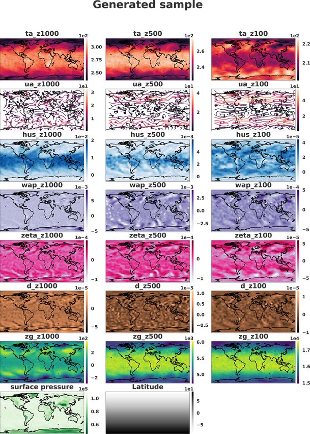
348                                                           C. Besombes et al.: Producing realistic climate data with GANs

cessfully learned to produce new realistic images. Several          mentation of the primitive equations on the sphere. An ar-
techniques developed for computer vision with GANs seem             chitecture is proposed for the generator and trained using an
promising for domains in the geosciences. Notable examples          approach based on the Wasserstein distance. A multivariate
of usage to date include Yeh et al. (2017) to do inpainting,        state is obtained by the transformation of a sample from a
where the objective is to recover a full image from an incom-       Gaussian random distribution in 64 dimensions by the gener-
plete one, Ledig et al. (2017) to do super resolution, or Isola     ator. Thanks to this sampling strategy, it is possible to com-
et al. (2017) to do image-to-image translation, where an im-        pute a climate as represented by the generator. Different met-
age is generated from another one, e.g., translate an image         rics are considered to compare the climate of the generator
that contains a horse into one with a zebra.                        with the true climate and to assess the realism of the gener-
   Data-driven approaches and numerical weather prediction          ated states. Because the distribution is known, the generator
are two domains that share important similarities. Watson-          provides a new way to explore the climate, e.g., simulating
Parris (2021) explains that both domains use the same meth-         the intensification of a weather situation or interpolating two
ods to answer different questions. This study and Boukabara         weather situations in a physically plausible manner.
et al. (2019) also show that numerical weather prediction              The article is organized as follows. The formalism of
contains lots of interesting challenges that could be tackled       WGAN is first introduced in Sect. 2 with the details of the
by machine-learning methods. It clarifies the growing litera-       proposed architecture. Then, Sect. 3 evaluates the ability of
ture about data-driven techniques applied to weather predic-        the generator to reproduce the climate of PLASIM with as-
tion. Scher (2018) used variational autoencoders to generate        sessment of the climate states that are produced by the gen-
the dynamics of a simple general circulation model condi-           erator. The conclusions and perspectives are given in Sect. 4.
tioned on a weather state. Weyn et al. (2019) trained a convo-
lutional neural network (CNN) on gridded reanalysis data in
order to generate 500 hPa geopotential height fields at fore-       2     Wasserstein generative adversarial network to
cast lead times up to 3 d. Lagerquist et al. (2019) developed a           characterize the climate
CNN to identify cold and warm fronts and a post-processing
                                                                    2.1    Parameterizing the climate of the Earth system
method to convert probability grids into objects. Weyn et al.
(2020) built a CNN able to forecast some basic atmospheric
                                                                    The Earth system is considered to be the solution of an evo-
variables using a cubed-sphere remapping in order to allevi-
                                                                    lution equation
ate the task of the CNN and impose simple boundary condi-
tions.                                                              ∂t χ = M(χ ),                                                (1)
   While there is a growing interest in using deep-learning
methods in weather impact or weather prediction (Reichstein         where χ denotes the state of the system at a given time and
et al., 2019; Dramsch, 2020), few applications have been de-        M characterizes the dynamics including the forcing terms,
scribed using GANs applied to physical fields in recent years       e.g., the solar annual cycle. While χ should stand for con-
(Wu et al., 2020). Notable examples include application to          tinuous multivariate fields, we consider its discretization in a
subgrid processes (Leinonen et al., 2019), to simplified mod-       finite grid so that χ ∈ X with X = Rn , where n denotes the
els such as the Lorenz ’96 model (Gagne et al., 2020) or to         dimension. Equation (1) describes a chaotic system. The cli-
data processing like satellite images (Requena-Mesa et al.,         mate is the set of states of the system along its time evolution.
2018). In particular, little is known about the feasibility of      It is characterized by a distribution or a probability measure,
designing and training a generator that would be able to pro-       denoted pclim .
duce multivariate states of a global atmosphere. A first diffi-        Obtaining a complete description of pclim is intractable
culty is to propose an architecture for the generator, with the     due to the complexity of natural weather dynamics and be-
specific challenge of handling the spherical geometry. Most         cause a climate database, pdata , is limited by numerical re-
of the neural network architectures in computer vision handle       sources and is only a proxy for this distribution.
regular two-dimensional images instead of images represent-            For instance, in the present study, the true weather dynam-
ing projected spherical images. Boundary conditions of these        ics M are replaced by the PLASIM model that has been
projections are not simple, as the spherical geometry also in-      time-integrated over 100 years of 6 h forecasts. Accounting
fluences the spread of the meteorological object as a function      for the spinup, the first 10 years of simulation are ignored.
of its latitude. These effects have to be considered in the neu-    Thus, the climate pclim is approximated from the resulting
ral network architecture. Another difficulty is to validate the     climate database of 90 years, pdata . The synthetic dataset is
climate resulting from the generator compared with the true         presented in detail in Sect. 3.1.
climate.                                                               Thus, pdata lives in the n-dimensional space X, but it is
   In this study, in order to evaluate the potential of GANs        non-zero only on an m-manifold M (where m  n) that can
applied to the global atmosphere, a synthetic climate is            be fractal. The objective is to learn a mapping
computed using the PLASIM global circulation simulator
(Fraedrich et al., 2005a), a simplified but realistic imple-        g : Z 7 −→ X                                                 (2)

Nonlin. Processes Geophys., 28, 347–370, 2021                                          https://doi.org/10.5194/npg-28-347-2021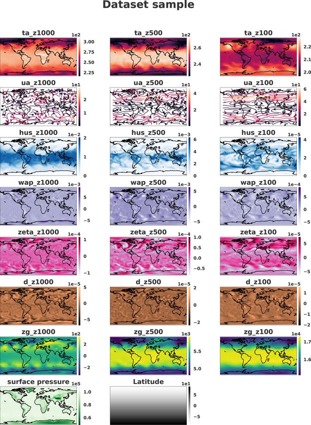
C. Besombes et al.: Producing realistic climate data with GANs                                                                       349

from Z = Rm , the so-called latent space, to X. Moreover, g          port theory and can be seen as the minimum work required
must transform a Gaussian N (0, Im ) to pdata ⊂ M.                   (in the sense of mass×transport) to transform the distribution
   The main advantage of such a formulation is to have a             pθ into the distribution pclim . Thus, the set 5(pθ , pclim ) can
function g that maps a low-dimensional continuous space Z            be seen as all the possible mappings, also called couplings, to
to M. This property could be useful in the domain of the             transport the mass from pθ to pclim . The Wasserstein distance
geosciences, notably in the climate sciences, where a high-          is a weak distance: it is based on the expectation, which can
dimensional space is ruled by important physical constraints         be estimated whatever the kind of distribution. Hence, the
and parameters.                                                      optimization problem is stated as
   Here the generator is a good candidate for learning the
physical constraints that make a climate state realistic with-       θ ∗ = argminθ W (pθ , pclim ),                                   (4)
out the need to run a complete simulation. The construction
                                                                     which leads to the WGAN approach.
of the generator is now detailed.
                                                                        One of the major advantages of the Wasserstein distance
2.2   Background on Wasserstein generative adversarial               is that it is real-valued for non-overlapping distributions. In-
      networks                                                       deed, the Kullback–Leibler (KL) divergence is infinite for
                                                                     disjoint distributions, and using it as a loss function leads to
To characterize the climate, we first introduce a simple Gaus-       a vanishing gradient (Arjovsky et al., 2017). The Wasserstein
sian distribution pz = N (0, Im ) of zero mean and covari-           distance does not exhibit vanishing gradients when distribu-
ance the identity matrix Im , defined on the space Z = Rm ,          tions do not overlap, as did the KL divergence in the original
called the latent space. The objective of an adversarial net-        GAN formulation.
work is to find a nonlinear transformation of this space Z              Unfortunately, the formulation in Eq. (3) is intractable. A
to X as written in Eq. (2) so that the Gaussian distribution         reformulation is necessary using the dual form discovered by
maps to the climate distribution, i.e., g# (pz ) = pclim , where     Kantorovich (Kantorovich and Rubinshtein, 1958). Refram-
g# denotes the push forward of a measure by the map g,               ing the problem as a linear programming problem yields
defined here as follows: for any measurable set E of X,
                                                                     W (pθ , pclim ) =        sup
g# (pz )(E) = pz (g −1 (E)), where g −1 (E) denotes the mea-                             f ∈1−Lipshitzian
surable set of Z that is the pre-image of E by g. The latent
space, Z, can be seen as an encoded climate space where                Ex∼pclim f (x) − Ex∼pθ f (x) ,                                 (5)
each point drawn from pz corresponds to a realistic climate          where 1 − Lipshitzian denotes the set of Lipshitzian func-
state and where the generator is the decoder. Looking for            tions f : Rn → R of coefficient 1, i.e., for any (x1 , x2 ) ∈ Rn ,
such a transformation is non-trivial.                                |f (x1 ) − f (x2 )| ≤ ||x1 − x2 ||, || · || being the Euclidian norm
   The search is limited to a family of transformations {gθ }        of Rn . For any 1 − Lipshitzian function f the computation of
characterized by a set of parameters θ. Thus, for each θ , the       Eq. (5) is simple: the first expectation can be approximated
nonlinear transform of the Gaussian pz by gθ is a distribu-          by
tion pθ . The goal is then to find the best set of parameters
θ ∗ such that θ ∗ = argminθ di(pθ , pclim ), where di is a mea-

                                                                     Ex∼pclim f (x) ≈ Ex∼pdata f (x) ,                                 (6)
sure of the discrepancy between the two distributions, so that
pθ ∗ approximates pclim . This method is known as genera-            where the right-hand side is computed as the empirical mean
tive learning, where gθ is implemented as a neural network           over the climate database pdata that approximates pclim in the
of trainable parameters θ . Note that, being a neural network,       weak sense Eq. (6). The second expectation can be computed
the resulting gθ is then a differentiable function.                  from the equality
   Even with this simplified framework, the search for an op-
                                                                     Ex∼pθ f (x) = Ez∼N (0;Im ) f (gθ (z)) ,                    (7)
timal θ is not easy. One of the difficulties is that the differen-
tiability of gθ requires the comparison of continuous distri-        where the expectation of the right-hand side can be approxi-
bution pθ with pclim , which is not necessarily a density on a       mated by the empirical mean computed from an ensemble of
continuous set. To alleviate this issue, Arjovsky et al. (2017)      samples of z which are easy to sample due to the Gaussianity.
introduced an optimization process based on the Wasserstein             However, there is no simple way to characterize the set
distance defined for the two distributions pclim and pθ by           of 1 − Lipshitzian functions, which limits the search for
                                                                   an optimal function in Eq. (5). Instead of looking at all
W (pθ , pclim ) =      inf     E(x,y) kx − yk ,                (3)
                 γ ∈5(pθ ,pclim )                                    1 − Lipshitzian functions, a family of functions {fw } param-
                                                                     eterized by a set of parameters w is introduced. In practice, it
where 5(pθ , pclim ) denotes the set of all joint
                                              R distributions        is engendered by a neural network with trainable parameters
γ (x, y) whose marginals are, respectively, y γ (·, dy) = pθ         w, called the critic.
    R
and x γ (dx, ·) = pclim . The Wasserstein distance, also called         Finally, if the weights of the network are constrained to a
the Earth mover distance (EMD), comes from optimal trans-            compact space W, which can be done by the weight-clipping

https://doi.org/10.5194/npg-28-347-2021                                          Nonlin. Processes Geophys., 28, 347–370, 2021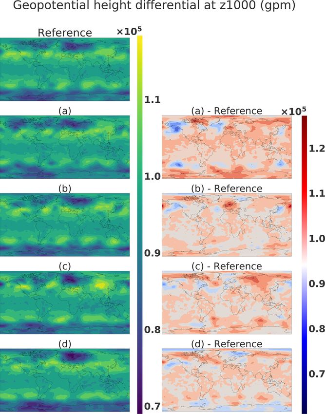
350                                                            C. Besombes et al.: Producing realistic climate data with GANs

method described in Arjovsky et al. (2017), then {fw }w∈W            parameter w̃(θq ) solution Eq. (9) (lines 3–11 in Algorithm 1).
will be K-Lipschitzian with K depending only on W and                In the second step, the critic is frozen and the generator is set
not on individual weights of the network. This yields                as trainable in order to compute θq+1 from Eq. (12) (lines
                                                               12–17 in Algorithm 1). Note that in Algorithm 1, the steep-
max Ex∼pdata fw (x) − Ez∼N (0;Im ) fw (gθ (z))                       est descent is replaced by an Adam optimizer (Kingma and
w∈W
                                                                  Ba, 2014), a particular implementation of stochastic gradient
      ≤      sup      Ex∼pdata f (x)
        f ∈1−Lipshitzian
                                                                     descent which has been shown to be efficient in deep learn-
                                                                  ing.
      − Ez∼N (0;Im ) f (gθ (z)) ,                            (8)        The following sections will aim to create a climate data
which tells us that the critic tends to the Wasserstein distance     generator from the WGAN method. The next section will
when trained optimally, i.e., if we find the max in Eq. (8)          describe the architecture of the network adapted to the com-
and if f is in (or close to) {fw }w∈W . The weight-clipping          plexity of the dataset used.
method was replaced by the gradient penalty method in Gul-
rajani et al. (2017) because it diminished the training quality      2.3   Neural network implementation
as mentioned in Arjovsky et al. (2017). Because it results
from a neural network, any function fw is differentiable, so         WGANs are known to be time-consuming to train, usually
that the 1−Lipshitzian condition remains to ensure a gradient        needing a high number of iterations due to the alternating as-
norm bounded by 1, i.e., for any x ∈ X, ||∇fw (x)|| ≤ 1. To          pect of the training algorithm between the critic and the gen-
do so, Gulrajani et al. (2017) have proposed computing the           erator. Our initial architecture used a simple convolutional
optimal parameter w̃(θ ) as the solution of the optimization         network for both, with a high number of parameters, but it
problem                                                              proved difficult to train a fitting multimodal distribution such
                                                                     as green distributions in the left panels in Fig. 15. That is why
w̃(θ ) = argsupw L(θ, w),                                    (9)     for this study a ResNet-inspired architecture (He et al., 2016)
                                                                     was chosen. The goal of the residual network is to reduce the
where L is the cost function                                         number of parameters of the network and avoid gradient van-
                                                                 ishing, which is a recurrent problem for deep networks that
L(θ, w) = Ex∼pdata fw (x) − Ez∼N (0;Im ) fw (gθ (z))
                     h                                               results in an even slower training.
                                    2 i
          + λEx̂∼p̂ ||∇fw (x̂)|| − 1 ,                 (10)             A network is composed of a stack of layers; when a spe-
                                                                     cific succession of layers is used several times, we can refer
with λ the magnitude of the gradient penalty and where x̂ is         to it as a block. The link between two layers is named a con-
uniformly sampled from the straight line between a sample            nection; a shortcut connection refers to a link between two
from pdata to a sample from pθ (line 8) of Algorithm 1. The          layers that are not successive in the architecture. A residual
optimal solution w̃(θ ) is obtained from a sequential method         block (Figs. 2 and 3) is composed with stacked convolution
where each step is written as                                        and a parallel identity shortcut connection. The idea is that it
                                                                     is easier to learn the residual mapping than all of it, so resid-
wk+1 = wk + βk ∇w L(θ, wk ),                                (11)     ual blocks can be stacked without observing a vanishing gra-
                                                                     dient. Moreover, a residual block can be added to an N -layer
where βk is the magnitude of the step. In an adversarial way,        network without reducing its accuracy because it is easier to
Eq. (10) could be solved sequentially, e.g., by the steepest         learn F (x) = 0 by setting all the weights to 0 than it is to
descent algorithm with an update given by                            learn the identity function. Residual blocks allow building of
θq+1 = θq − αq ∇θ W (pθq , pclim ),                         (12)     deeper networks without loss of accuracy.
                                                                        One should note that the PLASIM simulator is a spec-
where αq is the magnitude of the step. We chose to use the           tral model run on a Gaussian grid that consequently enforces
two-sided penalty for the gradient penalty method, as it was         the periodic boundary condition. In order to impose the pe-
shown to work well in Gulrajani et al. (2017). At conver-            riodic boundary condition in the generated samples, it was
gence, the Wasserstein distance is approximated by                   necessary to create a wrap padding layer, which takes multi-
                                                                   ple columns at the eastern side and concatenates them to the
W (pθ , pclim ) ≈ Ex∼pdata fw̃(θ) (x)                                western side and vice versa. In the critic, the wrap padding is
                                                                     only after the input, since the critic will discriminate the im-

                  − Ez∼N (0;Im ) fw̃(θ) (gθ (z)) .       (13)
                                                                     ages from the generator that are not continuous in the west–
Hence, the solution of the optimization problem Eq. (4) is           east direction. In the generator, the wrap padding layer is in
obtained from a sequential process composed of two steps,            every residual block; it is necessary because the reduced size
summarized in Algorithm 1. In the first step, the weights of         of the convolution kernel compared to the image size makes
the generator are frozen with a given set of parameters θq and       it more difficult for the network to extract features from both
the critic neural network is trained in order to find the optimal    sides of the image simultaneously. The north–south bound-

Nonlin. Processes Geophys., 28, 347–370, 2021                                           https://doi.org/10.5194/npg-28-347-2021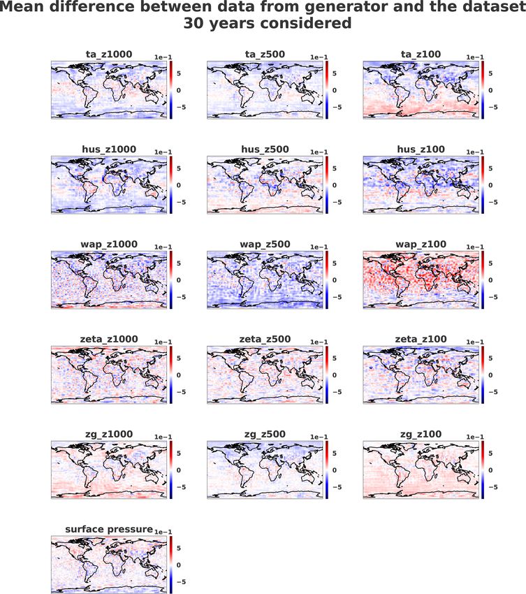
C. Besombes et al.: Producing realistic climate data with GANs                                                                   351

ary is padded by repeating the nearest line, called the nearest      in the critic architecture following Gulrajani et al. (2017); the
padding layer. In Figs. 1–5 padding layer arguments have             batch normalization changes the discriminator’s problem by
to be understood as (longitude direction, latitude direction),       considering all of the batch in the training objective, whereas
where the integer means the number of columns or rows to             we are already penalizing the norm of the critic’s gradient
be taken from each side and placed next to the other one; e.g.,      with respect to each sample in the batch.
Wrappadding (0, 3) means the output image is six columns
larger than the input. If the argument is not mentioned, then        2.3.2   Generator architecture
the arguments for wrap and nearest padding are (0, 1) and
(1, 0), respectively.                                                The input of the generator network (see Fig. 4) is an m-
                                                                     dimensional vector containing noise drawn from the nor-
2.3.1   Critic network                                               mal distribution N m (0, Im ) for the numerical experiment
                                                                     m = 64. The output of the generator has the shape of a sam-
The critic network input has the shape of a sample from the          ple of the dataset X ∈ Rnlat×nlon×nfield . The input is passed
dataset X ∈ Rnlat×nlon×nfield .                                      through a fully connected layer of output shape (8, 16, 128)
   Its output must be a real number because it is an approx-         and fed to residual blocks. The rest of its architecture is also
imation of the Wasserstein distance between the distribution         a residual network with a succession of modified convolu-
of the batch of images from the dataset and the one from             tional blocks (relative to the one in the critic network). Mod-
the generator that is being processed. The architecture ends         ifications of the convolutional block are the following.
with a dense layer of one neuron with linear activation. The
core of the structure is taken from the residual network and           1. An upsampling layer is added to increase the image size
can be seen in Fig. 1. After the custom padding layers men-               for some convolutional blocks.
tioned previously, the critic architecture is a classical residual
                                                                       2. Wrap and nearest padding layers are added in, respec-
network, starting with a convolution with 7 × 7 kernels, fol-
                                                                          tively, the west–east and north–south directions.
lowed by a maximum pooling layer to reduce the image size
and a succession of convolutional and identity blocks (Figs. 2         3. A batch normalization layer is present after convolu-
and 3). At each strided convolutional block, s = 2 in Fig. 3,             tional layers.
the image size is divided by a factor 2. It is equivalent to
a learnable pooling layer that can increase the result (Sprin-       One could argue that the ReLU activation function is not
genberg et al., 2014). Finally, an average pooling is done, and      differentiable in 0, but this is managed by taking the left
the output is fed to a fully connected layer of 100 neurons and      derivative in the software implementation. The study does
then to the output neuron. Batch normalization is not present        not claim that the network architectures used are optimal: the

https://doi.org/10.5194/npg-28-347-2021                                          Nonlin. Processes Geophys., 28, 347–370, 2021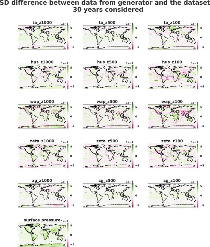
352                                                          C. Besombes et al.: Producing realistic climate data with GANs

                                                                   Figure 2. Residual identity block for the critic.
Figure 1. Critic architecture.

computational burden was too high to run a parameter sensi-
tivity study. Guidelines from Gulrajani et al. (2017) were fol-    Table 1. Hyperparameters for training step.
lowed, and the hyperparameters were adapted to the current
problem. It showcases an example of hyperparameters pro-                                         Network
ducing interesting results, and inspired readers are encour-        Hyperparameters                              Generator       Critic
aged to modify and improve this architecture.                       Iterations                                         30 000   150 000
                                                                    Batch size                                            128       128
2.3.3   Training parameters                                         Optimizer                                          Adam      Adam
                                                                    Initial learning rate (lr)                          1e−3      1e−3
For the training phase, the neural network’s hyperparameters        Learning rate decay every 3000 iterations             0.9       0.9
are summarized in Table 1. The training was performed on            Number of trainable weights                         1.5e6       4e6
an Nvidia Tesla V100-SXM2 with 32 GB of memory over                 λ in Eq. (10)                                                    10
2 d. The choice of the optimizer, initial learning rate, weight
of gradient penalty (λ in Eq. 10) and ratio between critic and

Nonlin. Processes Geophys., 28, 347–370, 2021                                          https://doi.org/10.5194/npg-28-347-2021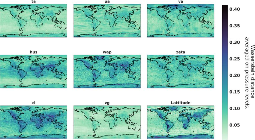
C. Besombes et al.: Producing realistic climate data with GANs                                                                       353

Figure 3. Residual convolutional block for the critic. If s is different
from 1, it is referenced as a strided convolutional block in Fig. 1.
                                                                           Figure 4. Generator architecture.

generator iteration was directly taken from Gulrajani et al.
(2017). The iterations mentioned in Table 1 are the number
of batches seen by each neural network.                                    distributions and should converge to 0. However, WGAN-
   The training loss in Fig. 6 was smoothed using exponential              GP is not yet proven to be locally convergent under proper
smoothing:                                                                 conditions (Nagarajan and Kolter, 2017); the consequence is
st = αyt + (1 − α) st−1 ,                                          (14)    that it can cycle around equilibrium points and never reach
                                                                           a local equilibrium. Condition on loss derivative is also dif-
where yt is the value of the original curve at index t, st is              ficult because of the instability of the GAN training proce-
the smoothed value at index t and α is the smoothing fac-                  dure. Consequently, a quality check using metrics adapted to
tor (equal to 0.9 here). An initial spinup of the optimization             the domain on which the GAN is applied is still necessary.
process tends to exhibit an increase in the loss of the first              Moreover, at the end of the training, a first experiment was
steps of the training phase before decreasing. This can be ex-             conducted to see whether the generations are present in the
plained by the lack of useful information in the gradient due              dataset. The histogram of the Euclidian distance divided by
to the initial random weights in the network. A decrease in                the number of pixels in one sample between one generation
the Wasserstein distance can be seen in Fig. 6, which indi-                and all of the dataset can be seen in Fig. 7. Here, one can
cates a convergence during the training phase, although it is              see that the minimum is around 0.8, which shows that the
possible to use the loss of the critic as a convergence criterion          generated image is not inside the dataset. This experiment
because the Wasserstein loss is used and has a mathematical                shows that the generator is able to generate samples without
meaning such as the distance between synthetic and real data               reproducing the dataset. It should be noted that in the WGAN

https://doi.org/10.5194/npg-28-347-2021                                                Nonlin. Processes Geophys., 28, 347–370, 2021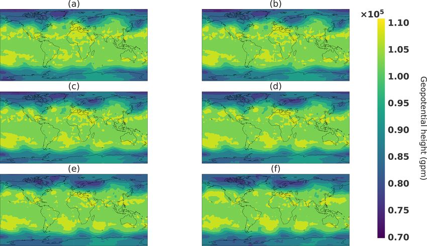
354                                                            C. Besombes et al.: Producing realistic climate data with GANs

                                                                     Figure 6. Smoothed version of the Wasserstein distance computed
                                                                     during the training. The vertical axis is in log scale.

                                                                     Figure 7. Two-norm distance between a generated sample and all
                                                                     the dataset samples.

Figure 5. Residual convolutional block for the generator. The up-
sampling layer can be removed if not necessary and is mentioned      Table 2. Variables used in the dataset.
when used in Fig. 4.
                                                                                       Variables
                                                                       Name                          Short name   Prognostic   Diagnostic
                                                                       Temperature (K)               ta           ×
framework, the generator never directly sees a sample from
                                                                       Eastward wind (m s−1 )        ua                        ×
the dataset.                                                           Northward wind (Pa s−1 )      va                        ×
   There are no stopping criteria for the training, and it was         Relative humidity (frac.)     hus          ×
stopped after 35 000 iterations in the interest of computa-            Vertical velocity (Pa s−1 )   wap                       ×
tional cost. It should be highlighted that the performance of          Vorticity (s−1 )              ζ            ×
generative networks and especially GANs is difficult to eval-          Divergence (s−1 )             d            ×
                                                                       Geopotential height (gpm)     zg           ×
uate. In the deep-learning literature, the quality of the images
                                                                       ln(surface pressure)          P                         ×
generated is assessed using a reference image dataset such as          Latitude (degree)             lat                       ×
ImageNet (Russakovsky et al., 2015) and computing the in-
ception score (IS) or the Fréchet inception distance (FID).

Nonlin. Processes Geophys., 28, 347–370, 2021                                              https://doi.org/10.5194/npg-28-347-2021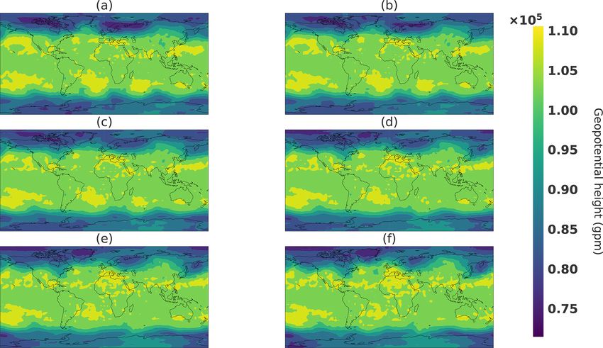
C. Besombes et al.: Producing realistic climate data with GANs                                                                   355

Both use the inception network trained on ImageNet: the IS              Each database sample is an 82-channel (nfield) two-
measures the quality and diversity of the images by classi-          dimensional matrix of size 64 (nlat) by 128 (nlon) pixels. The
fying them and measuring the entropy of the classification,          channels represent seven physical three-dimensional vari-
while the FID computes a distance between the features ex-           ables: the temperature (ta), the eastward (ua) and northward
tracted by the inception network and is more robust to GAN-          (va) wind, relative humidity (hus), vertical velocity (wap),
mode collapse.                                                       the relative vorticity (ζ ), divergence (d) and geopotential
   Because our study does not apply to the ImageNet dataset,         height (zg) at 10 pressure levels from 1000 to 100 hPa, plus
it is necessary to compute our own metrics. Section 3 pro-           the surface pressure (ps). Another channel was added to rep-
poses an approach for this kind of method in the domain              resent the latitude: it is an image going from −1 at the top of
of geosciences and more precisely the study of atmospheric           the image (North Pole) to 1 at the bottom (South Pole) in ev-
fields. Our main objective is to assess the fitting quality of       ery column. It was found that hard coding the latitude in the
the dataset climate distribution.                                    data improved the learning of physical constraints, allowing
                                                                     the network to be sensitive to the fact that the data are repre-
                                                                     sented by the equirectangular projection of the atmospheric
                                                                     physical fields, and, for example, the size of meteorologi-
3     Evaluation and exploration of the generator                    cal objects increases closer to the poles. Finally, the choice
                                                                     of having diagnostic variables in the dataset was to help the
The metrics by which the results will be analyzed are visual         post-processing, and assessment of their necessity requires
aspects, capacity to generate atmospheric balances and statis-       further research.
tics of the generations compared to climate distribution. For
the latter, the chosen metric is the Wasserstein distance. Be-       3.2   Comparison between climate dataset and
cause it is the same metric the generator has to minimize                  generated climate
during the training step, it seems a good candidate to as-
sess the training quality. One could argue that the network is       Our study aims to have a generator able to reproduce the cli-
overly trained on this metric; that is why we use other metrics      mate distribution present in the dataset made from the low-
such as mean and standard deviation differences and singular         resolution GCM PLASIM. This section proposes a way to
value decomposition to complete our analysis. Finally, be-           assess the quality of the distribution learned by the WGAN.
cause no trivial stop criteria are available, it is interesting to      The first required property for a weather generator is a
see where the magnitude of the Wasserstein distance is large         low computational cost compared to the GCM that produced
so as to diagnose some limitations of the trained generator          the data. Here the simulation with the GCM PLASIM took
that would provide some ideas of improvements.                       50 min for a 100-year simulation in parallel on 16 processors,
                                                                     whereas the generator took 3 min to generate 36 500 samples
3.1    Description of the synthetic dataset                          equivalent to a 100-year simulation on an NVIDIA Tesla V-
                                                                     100.
To create synthetic data, a climate model known as PLASIM               Each generated sample is compared with dataset samples.
(Fraedrich et al., 2005a) was used, which is a general circula-      Figures 8 and 9 show a sample where only the pressure lev-
tion model (GCM) of medium complexity based on a simpli-             els 1000, 500 and 100 hPa are represented for readability. It
fied general circulation model PUMA (Portable University             should be noted that the generated fields seem to be spatially
Model of the Atmosphere) (Fraedrich et al., 2005b). This             noisy compared to the dataset. The periodic boundary is re-
model based on primitive equations is a simplified analog            spected knowing that in the dataset the borders are located at
for operational numerical weather prediction (NWP) models.           the longitude 0◦ where no discontinuities can be observed. In
This choice facilitates the generation of synthetic data thanks      the figures, the image is translated in order to have Europe at
to its low resolution and reasonable computational cost. Dif-        the center of the image and to see whether some discontinu-
ferent components can be added to the model in order to im-          ities remain.
prove the circulation simulation such as the effect of ocean            In order to quantitatively assess the generator quality,
with sea ice, orography with the biosphere or annual cycle.          Figs. 10 and 11 show the mean and standard deviation pixel-
   A 100-year daily simulation was run at a T42 resolution           wise differences over 10 800 samples (equivalent to 30 years
(an approximate resolution of 2.8◦ ). We used orography and          of data) between normalized dataset and generations. It ap-
annual cycle parameterization; ocean and biosphere mod-              pears that fields where small-scale patterns are present are
elization were turned off in order to keep the dataset sim-          the most difficult to fit for the generator.
ple enough for our exploratory study. We removed the first              In order to go further in the analysis of the generated cli-
10 years in order to keep only the stationary part of the sim-       mate states, a singular value decomposition (SVD) was per-
ulation. These resulting 90 years of simulation constitute the       formed over 30 years of the dataset (renormalized over the
sampling of the climate distribution that we aim to reproduce.       30 years). Then the same number of generated data was con-
As preprocessing, each of the channels was normalized.               sidered and projected onto the five first principal components

https://doi.org/10.5194/npg-28-347-2021                                          Nonlin. Processes Geophys., 28, 347–370, 2021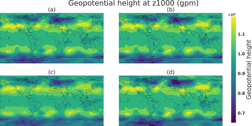
356                                                              C. Besombes et al.: Producing realistic climate data with GANs

Figure 8. Sample on three different pressure levels (1000, 500 and 100 hPa) taken from the dataset. The samples were horizontally transposed
in order to have Europe at the center of the images. Coastlines were added a posteriori for readability. Units available in Table 2.

of the SVD that represent 75 % of explained variance of the             structure of the original data is being preserved, and Fig. 12
dataset. In Fig. 12 the dot product is represented between              shows that the five eigenvectors are similar. One should note
SVD components derived from the dataset (ui )i∈{0,...,4} and            that the SVD algorithm used from Pedregosa et al. (2011)
another one derived from the generated data (vi )i∈{0,...,4} .          suffers from sign indeterminacy, meaning that the signs of
Figure 12 represents the cross-covariance matrix defined by             SVD components depend on the random state and the algo-
sij = ui · vj . Values close to 1 or −1 show that the eigen-            rithm. For this reason, we consider the dot product close to
vectors for both datasets (original and generated) are simi-            both 1 and −1. One should note that an inversion remains
lar. This is another way of assessing whether the covariance            between the components with indexes 3 and 4, which could

Nonlin. Processes Geophys., 28, 347–370, 2021                                               https://doi.org/10.5194/npg-28-347-2021
C. Besombes et al.: Producing realistic climate data with GANs 357
Figure 9. Sample on three different pressure levels (1000, 500 and 100 hPa) generated by the network. The samples were horizontally
transposed in order to have Europe at the center of the images to verify the quality of the periodic boundary. Coastlines were added a
posteriori for readability.
be explained by a difference of eigenvalue order (sorted in erations. This suggests a way of improving our method in
decreasing order) in each dataset that determines the order of future work.
eigenvectors. The fourth principal direction (index 3 in the Figure 15 shows the temperature (at the pressure level
figure) of the generated data represents more variation of the 1000 hPa) distribution at different pixel locations corre-
generated dataset than the same direction explains variation sponding to the red dots in Fig. 14. Different latitudes (42,
in the original dataset. Figure 13 shows clearly the inversion −2 and −70◦ ) were chosen to represent diverse distribu-
of the last principal components between the dataset and gen- tions. A value of Wasserstein distance is associated with each
plot, representing the distance between the two normalized
https://doi.org/10.5194/npg-28-347-2021 Nonlin. Processes Geophys., 28, 347–370, 2021358 C. Besombes et al.: Producing realistic climate data with GANs Figure 10. Mean error over 30 years of the normalized dataset and the same number of normalized generated samples on three different pressure levels (1000, 500 and 100 hPa). The samples were horizontally transposed in order to have Europe at the center of the images. Coastlines were added a posteriori for readability. distributions. It is notable that the Wasserstein distance in It follows that a good way to see the general statistics the context of GAN training was introduced by Arjovsky learned by the generator is to plot the Wasserstein distance et al. (2017) in order to avoid the mode collapse phenomenon for every pixel and for every variable. This result can be vi- where the generated samples produced by the GAN are rep- sualized spatially in Fig. 16, where we observe that certain resenting only one mode of the distribution. In Fig. 15, even variables are better fitted by the generator than others. The if the figure shows that some bimodal distributions remain figure also shows that areas with more variability such as land approximated by a unimodal distribution, the span of these areas and more precisely mountainous areas are the most dif- distributions covers the multiple modes of the targeted distri- ficult to fit. As a way to better interpret this metric, Fig. 17 bution. This explains why the higher Wasserstein distance in represents the distributions corresponding to the minimum the figure is in the top-left panel, since despite the bimodal- and maximum values of the metric. The distribution of the generated distribution the high temperature values do not Wasserstein distance can also be visualized grouped by pres- seem to be represented by the generated samples. sure level and type of variable in Fig. 18. The wap variable Nonlin. Processes Geophys., 28, 347–370, 2021 https://doi.org/10.5194/npg-28-347-2021
C. Besombes et al.: Producing realistic climate data with GANs 359
Figure 11. Standard deviation error over 30 years of the normalized dataset and the same number of normalized generated samples on
three different pressure levels (1000, 500 and 100 hPa). The samples were horizontally transposed in order to have Europe at the center of
the images. Coastlines were added a posteriori for readability.
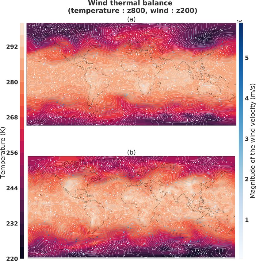
that represents the vertical velocity seems to be the one with 2006). The next two sections assess the ability of the genera-
the higher Wasserstein distance value. tor to reproduce the geostrophic and thermal wind balances.
3.3.1 Geostrophic balance
3.3 Analysis of the atmospheric balances
The geostrophic balance occurs at a low Rossby number
The previous subsection has shown the ability of the gen- when the rotation dominates the nonlinear advection term.
erator to engender weather situations and climate similar to Two forces are in competition: the Coriolis force, f k × u,
those of the simulated weather. However, geophysical fluids where k denotes the unit vector normal to the horizontal
are featured by multivariate fields that present known bal- (f is the Coriolis parameter and u is the wind) and the pres-
ance relations. Among these balances, the simplest ones are sure term −∇p 8, where 8 is the geopotential and where ∇p
the geostrophic and thermal wind balances (see, e.g., Vallis, denotes the horizontal gradient in the pressure coordinate.
https://doi.org/10.5194/npg-28-347-2021 Nonlin. Processes Geophys., 28, 347–370, 2021360 C. Besombes et al.: Producing realistic climate data with GANs
tial is found in the north of Europe. While the geopoten-
tial field is noisy (it is less smooth than in Fig. 19a), the
wind is again found to be nearly geostrophic, verifying the
geostrophic flow properties to within an error of 35 % (see
Fig. 20b). The geopotential and wind fields were projected
onto the solved dynamic truncation in order to remove the
subgrid component due to the noise in the output of the gen-
erator. Despite the truncation, the geostrophic approximation
seems to not be respected everywhere and could be a quanti-
tative metric to monitor in order to improve our method.
We find that weather situations generated from samples in
the latent space reproduce the geostrophic balance at an order
of approximation that is similar to the one of the real dataset.
This means that the generator is able to produce the realistic
multivariate link between the wind and the geopotential. This
property is essential in operational weather forecasting, e.g.,
in producing balanced fields in the ensemble Kalman filter.
3.3.2 Thermal wind balance
Figure 12. Scalar product of SVD components derived from a The thermal wind balance arises by combining the
dataset and generated data. geostrophic wind Eq. (15) and the hydrostatic approxi-
1
mations, ∂8∂p = − ρ , where ρ is the density (Vallis, 2006,
Sect. 2.8.4, p. 95): taking the derivative of Eq. (15) with re-
Asymptotically, the Coriolis force is then balanced by the spect to the pressure p makes the hydrostatic approximation
pressure term which leads to the geostrophic wind: appear, so that the vertical derivative of the geostrophic wind
can be written as
1
ug = k × ∇p 8. (15) ∂8 R
f = − k × ∇p T , (16)
∂p pf
The geostrophic flow is parallel to the line of constant
geopotential, and it is counterclockwise (clockwise) around where the ideal gas equation, p = ρRT , has been used.
a region of low (high) geopotential. The magnitude of the Equation (16) is the thermal wind balance that relates the
geostrophic wind scales with the strength of the horizontal vertical shear of the horizontal wind to the horizontal gradi-
gradient of geopotential Vallis (2006, Sect. 2.8.2, p. 92). ent of temperature. In particular, when the temperature falls
This asymptotic balance Eq. (15) is verified to within 10 % in the poleward direction, the thermal wind balance predicts
of error at mid latitude, that is, u = ug + uag , where the mag- an eastward wind that increases with height.
nitude of the ageostrophic wind, uag , is less than 0.1 of the Figure 21a and b show the vertical cross section of the
magnitude of the real wind u. zonal average of temperature and of the zonal wind for a
Figure 19a illustrates a particular boreal winter situation particular weather situation in the dataset, corresponding to
from the PLASIM dataset, focusing on the mid latitude and a boreal winter situation of the same weather situation rep-
presenting a low area of geopotential in the southwest of Ice- resented in Fig. 21: the temperature is higher in the South-
land. It appears that the wind is well approximated by the ern Hemisphere than in the Northern Hemisphere, with a
geostrophic wind, which is quantitatively verified in Fig. 20a strong horizontal gradient of temperature in latitude ranges
that shows the norm of the ageostrophic wind normalized by [−80◦ , −40◦ ] and [40◦ , 80◦ ]. At the vertical of the horizontal
the norm of the wind (that is, the relative error when ap- gradient of temperature, the wind is eastward and increases
proximating the wind by the geostrophic wind): the order with the height: this illustrates the thermal wind balance
of magnitude of the error is around 20 %. Properties of the which produces a strong curled jet at the vertical of the strong
geostrophic flow are visible, with a counterclockwise flow horizontal gradient of temperature as shown in Fig. 22a that
around the low geopotential. The wind is maximum where illustrates, for the same weather situation, the temperature
the horizontal gradient of geopotential is maximum, while at the bottom (800 hPa) with the horizontal wind at the top
its change in direction follows the trough. (200 hPa) of the troposphere.
A similar behavior can be observed in Fig. 19b, which il- The same illustrations are shown in Fig. 21c and d when
lustrates a weather situation selected from the render by the considering a generated situation, selected to correspond to a
generator of some samples in the latent space, so as to rep- boreal winter situation: the characteristics related to the ther-
resent a boreal winter situation. This time, a low geopoten- mal wind balance as observed before are found again. This
Nonlin. Processes Geophys., 28, 347–370, 2021 https://doi.org/10.5194/npg-28-347-2021C. Besombes et al.: Producing realistic climate data with GANs 361 Figure 13. Spatial components corresponding to principal components of SVDs applied to the dataset and the generated samples. results in the generator being able to render a weather sit- putted by the generator, which is beyond the scope of this uation that reproduces the thermal wind balance. Moreover, study. For example, it would be interesting to assess whether Fig. 23 shows the thermal wind balance averaged on 30 years other inter-variable balances are present, such as the ω equa- for the dataset (Fig. 23a) and generations (Fig. 23b); both are tion or vertical structures. Note that adding advanced diag- very similar. nostic fields in the output of the generator could be investi- This section has shown the ability of the generator to gated to improve the realism. reproduce some important balances present in the atmo- sphere. In particular, the generator is able to produce mid- latitude cyclones whose velocity field is in accordance with the geostrophic balance. The authors emphasize that it is nec- essary to conduct more analysis of the weather situations out- https://doi.org/10.5194/npg-28-347-2021 Nonlin. Processes Geophys., 28, 347–370, 2021
362                                                              C. Besombes et al.: Producing realistic climate data with GANs

Figure 14. Location from where the temperature distributions are plotted in Fig. 15. The Wasserstein distance value associated for each plot
was computed on normalized data.

Figure 15. Temperature distribution at different locations for 5000 samples from dataset (green) and generated (blue).

3.4   Exploration of the latent space structure and its                 trained, then each sample generated with it should represent
      connection to the climate                                         a typical weather situation. It is hard to figure out what the at-
                                                                        tractor of the climate is. However, the geometry of the Gaus-
An exploratory study was done on the property of the la-                sian in high dimension being known, it is easy to characterize
tent space and its consequence in the climate space in regard           the climate in the latent space.
to climate domain problematics. If the generator is perfectly

Nonlin. Processes Geophys., 28, 347–370, 2021                                               https://doi.org/10.5194/npg-28-347-2021
C. Besombes et al.: Producing realistic climate data with GANs 363
Figure 16. Wasserstein distance between 5000 datasets and generated samples on each pixel and each channel.
Figure 17. Distributions with the higher (a) and lower (b) Wasser-
stein distances computed on normalized data. The coordinates of
corresponding pixels are, respectively, in latitude and longitude.
3.4.1 Geometry of the normal distribution
For a normal law in the high dimension space Z = Rm , i.e.,
with m larger than 10, the distributions√of the samples are
all located in a spherical shell of radius m and of thickness
on order √1 (see, e.g., Pannekoucke et al., 2016). Because
2
the covariance matrix Im is a diagonal of constant variance, Figure 18. Wasserstein distance between 5000 datasets and gener-
no direction of Rm is privileged, leading to an isotropic dis- ated samples on each pixel grouped by pressure height (a) or vari-
tribution of the direction of the sampled vectors: their unit ables (b).
directions uniformly cover the unit sphere. Another property
https://doi.org/10.5194/npg-28-347-2021 Nonlin. Processes Geophys., 28, 347–370, 2021364 C. Besombes et al.: Producing realistic climate data with GANs
Figure 24 illustrates this low-dimensional representation
of an ensemble of 10 000 samples of the normal law in di-
mension m = 64. For instance, points A and B represent two
independent
√ samples: their distance to the origin is closed to
m = 8, and their angle is closed to π2 . While m = 64 can
be considered a very small dimension, it appears that the dis-
tribution of the
√ point’s distance to the origin is well fit by the
Gaussian N ( 64, 21 ) (see inset figure in Fig. 24). Hence, it
results that for this dimension, the interpretation of a Gaus-
sian distribution as a spherical shell applies, with interesting
consequences for extremes or typical states. A typical sample√
of this normal law is a point near the sphere of radius 64,
while an extreme √ sample has a norm lying in the tails of the
distribution N ( 64, 12 ).
This suggests evaluating whether the extremes of the latent
space correspond to those of the meteorological space.
Figure 19. Geostrophic and ageostrophic wind derived from geopo- 3.4.2 Connection between extremes in the latent and
tential at 500 hPa. Situation taken from dataset (a) and gener- physical spaces
ated (b).
Knowing what are the extremes in the latent space might be
helpful to determine what are the extremes of the climate,
at least to determine what are extreme situations closed to a
given state.
For any sample in the latent space,
√ say point A, we can
construct the point on the sphere m along the same direc-
tion of A, A, which can be considered the most likely typical
state near A. Along the same direction of A, we can also
construct
√ the extreme situations A± whose distances to the
3
origin, m ± √ , lay, respectively, in the left and right tails
2 √
of the Gaussian distribution N ( m, 12 ).
Figure 25 represents the weather situation generated from
a randomly drawn latent vector from a 64-dimensional Gaus-
sian N (0, 1) sample A (Fig. 25a). Panel (a) represents a la-
tent vector with a Euclidian norm equal to 7.69, close to the
mean of the radial distribution of the hypersphere mentioned
in Sect. 3.4.1. In the climate space this sample shows a me-
Figure 20. Relative error in the norm between geostrophic wind teorological object above northern Europe in the shape of a
and normal wind shown in Fig. 19 for the situation taken from geopotential minimum which can be interpreted as a storm.
dataset (a) and generated (b). This sample is the same as the one represented in Figs. 19b,
21b, and 22b.
The most likely typical state A (Fig. 25b) is the radial pro-
is that the angle formed by two sampled vectors is approx- jection of the latent vector A onto the mean of the radial dis-
imately of magnitude π2 : two random samples are orthogo- tribution; thus, its Euclidian norm is equal to 8. Because sam-
nal. These are simple consequences of the central limit the- ple A has a norm close to sample B, the weather situations
orem which predict, for instance, that the distance of a sam- are very similar at the geopotential height at z1000. This is an
ple √
to the center of the sphere is asymptotically the Gaussian expected effect because by construction of the generator the
N ( m, 12 ). input space is continuous, so two points in the latent space
Considering these properties, one can introduce a must be similar. Extreme situation A± along the direction
two dimensional pseudo-representation which preserves the of A is represented in Fig. 25c and d. Both panels shows
isotropy of the distribution as well as the distribution to the clear differences in the geopotential height. First the panel
origin: a random sample vector x = (x1 , x2 , · · ·, xm ) in Rm is (Fig. 25c) shows a decrease in the storm located above north-
represented by the projection P2 (x) = ||x|| q 21 2 (x1 , x2 ), ern Europe; the same effect is visible in the south of South
x1 +x2 America. However, the weather situation is very similar to
where || · || stands for the Euclidian norm in Rm . Fig. 25a. By contrast, Fig. 25d represents a deeper geopoten-
Nonlin. Processes Geophys., 28, 347–370, 2021 https://doi.org/10.5194/npg-28-347-2021C. Besombes et al.: Producing realistic climate data with GANs 365
Figure 21. Temperature (K) and zonal wind (m s−1 ) latitude zonals from a boreal winter situation: the thermal wind balance. Left panels
correspond to a situation taken from the dataset. (a) Zonal temperature and (c) zonal wind. Right panels correspond to a situation taken from
the generator. (b) Zonal temperature and (d) zonal wind.
generator aims to map a distribution (64-dimensional Gaus-
sian in the latent space) to another (weather distribution in
the PLASIM physical space). Rare events exist in the latent
space on the tails of the Gaussian distribution’s potentially
extreme weather situations. One of the ways to do a such
mapping is to use the radial direction to represent high- or
low-probability states of the climate. An important conclu-
sion is that, for a given situation, the most likely state and the
extremes are interesting physical states. This could open new
possibilities to study an extreme situation close to a given
one, which is an important topic, e.g., for insurance or to
improve the study of high weather impact in ensemble fore-
casting.
The link of the animation of such interpolation is available
on GitHub1 of the project.
3.4.3 Interpolation in the latent space
Even if there are no dynamics in the latent space, which
makes it impossible to construct a prediction from this space,
we can consider how to interpolate two latent states. A naive
answer is to compute the linear interpolation between two
Figure 22. Thermal wind balance from the boreal winter situation samples of the latent space A and B,
shown in Fig. 21: (a) sample from the dataset; (b) sample generated
by the generator. The temperature (K) is from pressure level 800 hPa Mt = G ((1 − t)A + tB) , (17)
and the wind (m s−1 ) from 200 hPa.
which results in the red chordal illustrated in Fig. 24. The
chordal interpretation highlights a major drawback of the lin-
ear interpolation: middle points of the chordal are extremes;
tial height minimum at the pre-existing storm of sample A.
these intermediate points should not correspond to typical (or
Thus, Fig. 25 seems to show a certain structure of the latent
even physically realizable) weather situations.
space generator where the radial direction could represent the
strength of the meteorological objects such as storms above 1 https://github.com/Cam-B04/Producing-realistic-climate-data-
Europe, for example. It could be explained by the fact that the with-GANs (last access: 15 January 2021)
https://doi.org/10.5194/npg-28-347-2021 Nonlin. Processes Geophys., 28, 347–370, 2021366 C. Besombes et al.: Producing realistic climate data with GANs
Figure 23. Temperature (K) and zonal wind (m s−1 ) latitude zonals averaged on the 30-year subsample. Left panels correspond to a situation
taken from the dataset: (a) zonal temperature and (c) zonal wind. Right panels correspond to a situation taken from the generator: (b) zonal
temperature and (d) zonal wind.
Figure 25. Generations obtained by radial interpolation in the latent
space. Panel (a) is the image corresponding to a randomly drawn la-
tent vector A (two-norm: 7.69), (b) is its projection onto the mean
of the same direction A (two-norm: 8.0), and (c) and (d) are the
projection onto, respectively, inferior A− (two-norm: 5.87) and su-
perior A+ (two-norm: 10.12) 1 % quantile (see Fig. 24).
So as to preserve the likelihood of the interpolated weather
situations, it is better to introduce a spherical interpolation.
This kind of interpolation has also been used in image pro-
cessing, where, e.g., White (2016) uses the formula
Figure 24. Pseudo-spherical metaphorical representation of 10 000
sin ((1 − t)θ) sin (tθ)
Mt = G A+ B , (18)
samples of the normal distribution in Rm with m = 64 and the dis- sin θ sin θ
tribution of the distance of samples to the center of the spherical
shell. For a sample A, A± denotes two extreme situations along the where θ is the angle A, dB and for t ∈ [0, 1] such as M0 =
direction of A. Any second sample B, typical of the distribution, G(A) and M1 = G(B).
appears orthogonal to A. The inset figure represents the radial dis- This interpolation will connect point A to point B within
tribution compared with the
√ asymptotic central limit theorem (CLT)
the spherical shell of typical states, as illustrated by the or-
Gaussian distribution N ( m, 21 ) (thin red curve). ange curve line in Fig. 24. Figure 26 shows snapshots of
the climate generated from a spherical interpolation in the
latent space between sample A and another random sample
Nonlin. Processes Geophys., 28, 347–370, 2021 https://doi.org/10.5194/npg-28-347-2021You can also read