Acoustic velocity measurements for detecting the crystal orientation fabrics of a temperate ice core - The Cryosphere
←
→
Page content transcription
If your browser does not render page correctly, please read the page content below
The Cryosphere, 15, 3507–3521, 2021
https://doi.org/10.5194/tc-15-3507-2021
© Author(s) 2021. This work is distributed under
the Creative Commons Attribution 4.0 License.

Acoustic velocity measurements for detecting the crystal
orientation fabrics of a temperate ice core
Sebastian Hellmann1,2 , Melchior Grab1,2 , Johanna Kerch3,4 , Henning Löwe5 , Andreas Bauder1 , Ilka Weikusat3,6 , and
Hansruedi Maurer2
1 Laboratory of Hydraulics, Hydrology and Glaciology (VAW), ETH Zurich, Zurich, Switzerland
2 Institute
          of Geophysics, ETH Zurich, Zurich, Switzerland
3 Alfred-Wegener-Institut Helmholtz-Zentrum für Polar- und Meeresforschung, Bremerhaven, Germany
4 GZG Computational Geoscience, Georg-August University, Göttingen, Germany
5 WSL Institute for Snow and Avalanche Research SLF, Davos, Switzerland
6 Department of Geosciences, Eberhard Karls University, Tübingen, Germany

Correspondence: Sebastian Hellmann (sebastian.hellmann@erdw.ethz.ch)

Received: 11 January 2021 – Discussion started: 4 February 2021
Revised: 20 June 2021 – Accepted: 23 June 2021 – Published: 28 July 2021

Abstract. The crystal orientation fabric (COF) in ice cores          are available within the sampling volume, and both meth-
provides detailed information, such as grain size and distribu-      ods provide consistent results in the presence of a similar
tion and the orientation of the crystals in relation to the large-   amount of grains. We also explore the limitations of ultra-
scale glacier flow. These data are relevant for a profound           sonic measurements and provide suggestions for improving
understanding of the dynamics and deformation history of             their results. These ultrasonic measurements could be em-
glaciers and ice sheets. The intrinsic, mechanical anisotropy        ployed continuously along the ice cores. They are suitable to
of the ice crystals causes an anisotropy of the polycrystalline      support the COF analyses by bridging the gaps between dis-
ice of glaciers and affects the velocity of acoustic waves           crete measurements since these ultrasonic measurements can
propagating through the ice. Here, we employ such acoustic           be acquired within minutes and do not require an extensive
waves to obtain the seismic anisotropy of ice core samples           preparation of ice samples when using point-contact trans-
and compare the results with calculated acoustic velocities          ducers.
derived from COF analyses. These samples originate from
an ice core from Rhonegletscher (Rhone Glacier), a tem-
perate glacier in the Swiss Alps. Point-contact transducers
transmit ultrasonic P waves with a dominant frequency of             1   Introduction
1 MHz into the ice core samples and measure variations in
the travel times of these waves for a set of azimuthal angles.       Improved glacier flow models require a profound knowledge
In addition, the elasticity tensor is obtained from laboratory-      on sub- and englacial processes and the properties governing
measured COF, and we calculate the associated seismic ve-            these processes. The data for studying englacial processes are
locities. We compare these COF-derived velocity profiles             usually derived either from borehole measurements or from
with the measured ultrasonic profiles. Especially in the pres-       ice core analyses. These ice core analyses provide useful
ence of large ice grains, these two methods show signifi-            physical properties, such as elastic parameters, density, elec-
cantly different velocities since the ultrasonic measurements        tric conductivity, and permittivity (e.g. Freitag et al., 2004;
examine a limited volume of the ice core, whereas the COF-           Wilhelms, 2005). Most of these properties are anisotropic
derived velocities are integrated over larger parts of the core.     in ice cores because the physical properties of a single ice
This discrepancy between the ultrasonic and COF-derived              crystal vary along its principal axes, and the crystals usu-
profiles decreases with an increasing number of grains that          ally exhibit preferential orientations under deformation. Fur-
                                                                     thermore, ice cores provide geometric details on the ice mi-

Published by Copernicus Publications on behalf of the European Geosciences Union.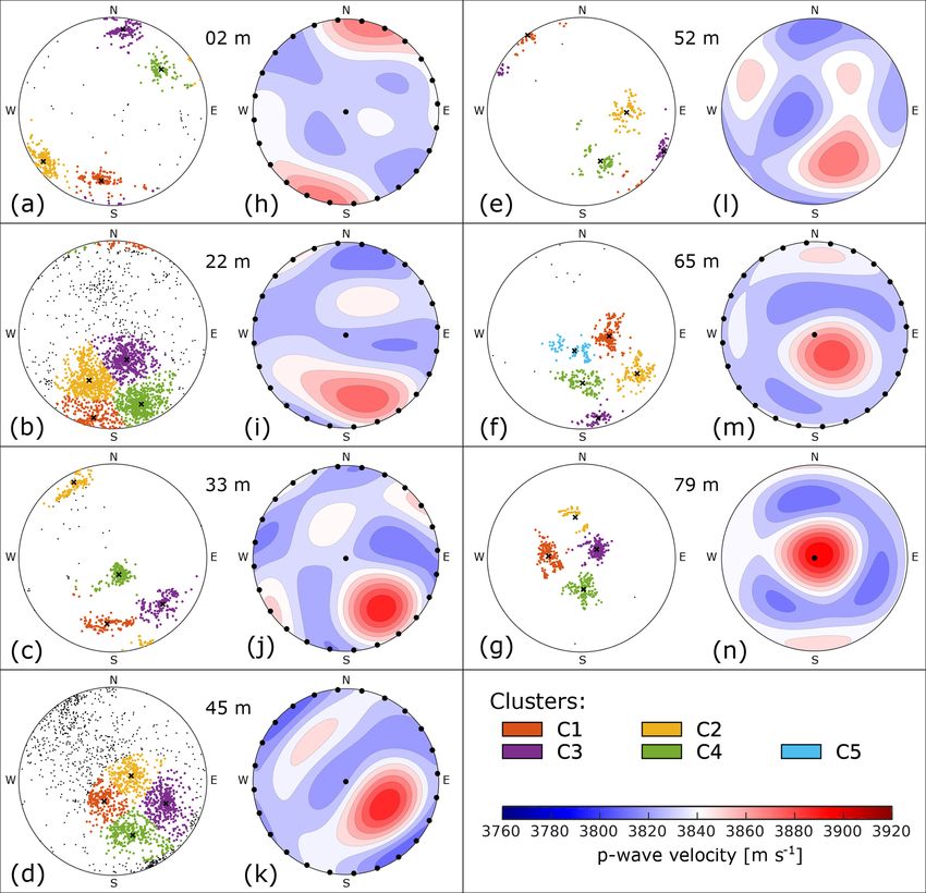
3508                                                                S. Hellmann et al.: Velocity measurements for COF detection

crostructure, such as grain size and shape, and information             2021). The large grain size in temperate ice may also affect
on crystal orientation. The derived crystal orientation fab-            the aforementioned ultrasonic measurements as a result of
ric (COF) describes the orientation of the ice grains’ c axes,          fewer grains within the ice core volume.
which are the symmetry axes of the individual ice monocrys-                Different geophysical methods have been employed to ex-
tals in the polycrystalline material. The COF is governed by            plore the horizontal extension of the major layers of changing
the stress field and the ice deformation and thus preserves the         COF (e.g. Bentley, 1975; Blankenship and Bentley, 1987;
ice flow history of a glacier or ice sheet (Budd, 1972; Azuma           Matsuoka et al., 2003; Drews et al., 2012; Diez et al., 2015;
and Higashi, 1984; Alley, 1988). It is also an indicator for the        Picotti et al., 2015). Surface geophysical methods provide
internal ice structure at the ice core location, which allows for       easy access to the dominant COF layers in ice sheets (Bris-
a classification of the ice as “soft” or “hard” depending on the        bourne et al., 2019; Jordan et al., 2019). For more detailed
direction of the strain rates relative to the COF (e.g. Budd and        investigations, borehole sonic experiments (Bentley, 1972;
Jacka, 1989; Faria et al., 2014). Such information is crucial           Pettit et al., 2007; Gusmeroli et al., 2012) are suitable meth-
for improving glacier flow models that consider anisotropy              ods to analyse the COF in a (sub-)metre range. Kluskiewicz
effects (Alley, 1992; Azuma, 1994). For example, informa-               et al. (2017) have successfully demonstrated the advantages
tion on the anisotropic ice flow dynamics of a glacier has              of this method to analyse the COF in ice core boreholes in
successfully been incorporated in ice flow models by Gillet-            western Antarctica. For all these experiments, the seismic
Chaulet et al. (2005), Placidi et al. (2010), and Graham et al.         velocity is considered as the relevant measurement param-
(2018).                                                                 eter. Therefore, Maurel et al. (2015) advanced a theoretical
   For the analysis of the COF, thin sections of ice (≈ 350 µm          approach of Nanthikesan and Sunder (1994) to calculate the
thick) are manually prepared from ice core samples and fi-              seismic velocities from given COF to compare them with di-
nally measured with an automated fabric analyser (e.g. Wil-             rectly measured sonic velocities in boreholes. Diez and Eisen
son et al., 2003; Peternell et al., 2009). This processing work-        (2015) developed a very similar theoretical framework to cal-
flow is state of the art, but it is labour-intensive and usu-           culate the expected seismic velocities for a given COF pat-
ally yields only discrete measurements along the entire ice             tern (including cone, thick, and partial girdle fabrics as they
core. Therefore, other methods have been proposed in the last           are typically found in polar ice cores) for comparison with
decades. Initial attempts to develop new methods were con-              surface geophysical investigations. This was extended to a
ducted throughout the late 1980s and early 1990s. Langway               more general framework by Kerch et al. (2018) for any given
et al. (1988) developed a tool that uses P waves for COF de-            COF.
tection. This methodology required a preparation of the core               A direct comparison of the measured and calculated veloc-
samples to obtain plane-parallel surfaces on which the plane            ities is still limiting as the measured data may be affected by
transducers could be attached. Later, Anandakrishnan et al.             macro-structural features such as crevasses, fractures, chang-
(1994) advanced this methodology by developing a concept                ing ice porosity due to air bubbles, or meltwater within the
with shear waves that reduced the labour-intensive prepa-               ice matrix. In order to avoid all these limitations, direct ultra-
ration of the core samples. Recently, Gerling et al. (2017)             sonic measurements along an ice core, from which the COF
used travel time differences of acoustic waves to determine             is usually derived, could be employed and may provide the
the elastic modulus of snow. During the past years, mod-                best agreement between COF-derived and measured acous-
ern non-contacting laser ultrasound acquisition systems have            tic velocities. Such a comparison of ultrasonic measurements
been developed for different purposes, such as investigating            with COF-derived velocities is the aim of this study. We
stratigraphic layering of ice cores for dating (Mikesell et al.,        obtain seismic velocities from ultrasonic measurements on
2017). These methods investigate the elastic parameters of              ice core samples from the temperate Rhonegletscher (Rhone
the ice. Since elastic parameters and COF are directly related,         Glacier) in Switzerland. We already analysed the actual COF
the methods can also be employed for COF analyses.                      of these ice core samples in a recent study (Hellmann et al.,
   Important factors to consider when designing a measure-              2021) and use the framework of Kerch et al. (2018) to cal-
ment procedure for COF analyses are grain size and shape                culate the COF-derived seismic velocity profiles. X-ray to-
of the ice samples or the air bubble distribution, which in-            mography analyses are incorporated to account for air bub-
fluences the density of the ice. The grain size and shape dif-          bles that are still affecting this comparison. We demonstrate
fer significantly between cold ice and temperate ice. Cold              the potential of our ultrasonic method applied to an ice core
ice typically has larger quantities of small (millimetre-sized)         to directly link to the complementary fabric measurements
grains, whereas temperate ice has significantly fewer grains,           acquired with polarisation microscopy and provide sugges-
but they are larger, with their diameter being up to sev-               tions for further improvements. To our knowledge, this is the
eral centimetres. Furthermore, the grains in temperate ice              first comparative study of COF-derived and ultrasonic veloc-
are often more irregularly shaped and interlocked and con-              ity analyses on temperate ice.
sequently appear as several individual grains within the thin
sections. This often leads to a misinterpretation of the actual
COF (Budd, 1972; Hooke and Hudleston, 1980; Monz et al.,

The Cryosphere, 15, 3507–3521, 2021                                                         https://doi.org/10.5194/tc-15-3507-2021
S. Hellmann et al.: Velocity measurements for COF detection 3509
2 Data acquisition and methods fel equation (e.g. Tsvankin, 2001, chap. 1.1.2). According to
Maurel et al. (2016), this approach for an effective elastic-
2.1 Ice core fabric data ity tensor provides more accurate results (at least for some
specific textures) than the complementary velocity averag-
For our velocity investigations we used an ice core drilled ing method (i.e. calculating the velocities for the individual
on Rhonegletscher, Central Swiss Alps. The ice core was crystals and computing the average velocity for the polycrys-
drilled in August 2017 with a recently developed thermal talline medium afterwards). Here, we only summarise the
drilling technique suitable for temperate ice (Schwikowski key points for calculating the effective elasticity tenor:
et al., 2014). An 80 m long ice core was retrieved in the
– This approach is based on an earlier study of Diez
ablation area of the glacier (46◦ 35.2200 N, 008◦ 23.2680 E;
and Eisen (2015). However, the framework of Diez and
2314 m a.s.l. in 2017). In the location of the drilled ice core,
Eisen (2015) relies on particular COF patterns, such as
the glacier flows from a northwestern (≈ 335◦ ± 10◦ ) to a
a thick and partial girdle or a single maximum structure,
southeastern direction.
and their representation through the eigenvalues of the
Immediately after extracting the ice core, it was stored
orientation tensor. Kerch et al. (2018) do not presume
at −30 ◦ C. This caused any water-filled pores within the
specific COF patterns, which makes it most suitable for
ice matrix to freeze. Seven samples (0.5 m length each)
our dataset.
along the ice core were analysed at Alfred Wegener In-
stitute Helmholtz Centre for Polar and Marine Research – It then considers the elements of a monocrystal tensor
(AWI), Bremerhaven, in order to obtain a comprehensive Cm precisely determined in laboratory experiments. In
COF dataset. For each sample, 8 to 12 horizontal and ver- our study, we used the elasticity tensor of Bennett,
tical thin sections (covering three perpendicular planes) from
14.06 7.15 5.88 0 0 0
two adjacent ice core segments (see Fig. 1c) were prepared. 7.15 14.06 5.88 0 0 0
The COF was then analysed with polarised light microscopy
5.88 5.88 15.24
0 0 0
(Peternell et al., 2009). We employed the automatic fabric Cm =
0 0 0 3.06 0 0
analyser G50 from Russell-Head Instruments (e.g. Wilson
0
0 0 0 3.06 0
et al., 2003) and the software cAxes (Eichler, 2013) to ob-
0 0 0 0 0 3.455
tain a comprehensive fabric dataset for each ice core sample.
The results of this COF analysis are presented in Fig. 2a to g × 109 N m−2 ,
and further details can be found in Hellmann et al. (2021).
calculated by Bennett (1968) for T = −10 ◦ C. This pro-
vides the best agreement between our calculated and
2.2 Seismic velocities from COF
measured data in both our study and in earlier experi-
ments (Diez et al., 2015, their Table 1).
The hexagonal crystal structure of an ice monocrystal causes
an anisotropy in its elastic parameters and therefore affects – For each ice grain i the monocrystal tensor Cm is trans-
the propagation velocity of seismic waves. As a result of the formed into
crystallographic symmetry, the acoustic velocity parallel to
the c axis, which corresponds to the optical axis perpendic- Crot T T
m (i) = Rϑ (i)Rϕ (i)Cm Rϕ (i)Rϑ (i),
ular to the basal planes of the ice crystal lattice (e.g. Cuffey where Rϑ is the rotational matrix around the verti-
and Paterson, 2010) and differs significantly from the veloc- cal axis, Rϕ is the rotational matrix around geographic
ity in direction of the basal plane. This seismic anisotropy north, and ϑ and ϕ are the azimuth and the colatitude
of an ice crystal is fully described by the fourth order elas- angle of the grain i, respectively. This aligns the elas-
ticity tensor Cij kl , i, j, k, l = 1, 2, 3 (e.g. Aki and Richards, ticity tensor with the coordinate system of the ice core
2002). The velocity of an acoustic wave with any inclina- (transformation of the coordinate system).
tion and azimuthal direction can be calculated analytically
(Tsvankin, 2001) provided the mass density of ice is known. – The rotated monocrystal tensors are summed up ele-
Due to the symmetry relations (Voigt, 1910) the 81 un- mentwise as
known elements of the tensor can be reduced to 21 elements. XnG
The hexagonal symmetry of ice further reduces the number Cp = wG (i) Crot
m (i),
of independent constants to five for a monocrystal. For the i=1
determination of a representative elasticity tensor for a poly- thereby assuming a superposition of all nG grains and
crystalline medium, we follow the approach of Kerch et al. their respective properties. The relative grain sizes are
(2018). used as weighting factors wG (i) for each grain. The re-
The theoretical framework calculates the effective elastic- sulting polycrystalline tensor does not have a hexagonal
ity tensor and derives the seismic velocities from this ten- structure anymore but a triclinic structure with 21 inde-
sor. Then, the velocities are derived by solving the Christof- pendent elements.
https://doi.org/10.5194/tc-15-3507-2021 The Cryosphere, 15, 3507–3521, 2021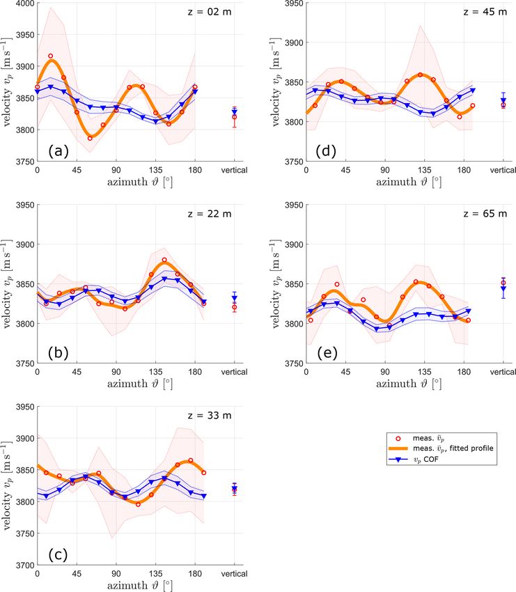
3510                                                               S. Hellmann et al.: Velocity measurements for COF detection

Figure 1. (a) Schematic experimental set-up for ultrasonic measurements on the ice core with tools and devices (amplifiers not shown).
(b) Example dataset of seismic traces for horizontal measurements. (c) The segmentation of two adjacent ice core segments depicting the
position of the ultrasonic and COF analyses.

  – With the known elastic properties, the Christoffel equa-              The orientation of each individual ice core segment was
    tion provides the link to analytic solutions for acoustic          marked at the time of drilling based on mechanical onsets
    velocities vp , vSH , and vSV .                                    and supporting magnetometric measurements. This ensures
                                                                       a comparison between COF, ultrasonic measurements, and
The calculations for the polycrystalline tensor and acoustic           glacier flow at all depths. The temperature for the ultrasonic
velocities are described in more detail in Maurel et al. (2015)        measurements was chosen to be at T = −5 ◦ C. This is a com-
and Kerch et al. (2018).                                               promise between temperate ice conditions and a controlled
   The seismic velocities can be calculated from the elastic-          cold environment in order to avoid melting effects during the
ity tensor or the inverse compliance tensor. Both approaches           measurement.
provide velocity profiles oscillating around an upper (Voigt              An ultrasonic point-contact (PC) transducer transmitted an
bound) and lower (Reuss bound) mean velocity (Hill, 1952).             acoustic signal into the ice. This signal was recorded by a
We calculated the seismic velocities from both tensors to ob-          second transducer on the opposite side of the core. In the
tain these upper and lower bounds of the potential velocity            current experimental set-up only measurements parallel and
range and further derived the velocity profile from the Hill           perpendicular to the vertical axis of the ice core (colatitude
tensor (the mean of elasticity and compliance tensor). This            ϕ = 0 and 90◦ ) were considered. The azimuthal coverage for
analytic solution is in agreement with the numerical approach          ϕ = 90◦ was 1ϑ = 15 between 0 and 345◦ .
implemented in the Matlab toolbox MTEX (e.g. Mainprice                    Figure 1a shows the experimental set-up that consists of
et al., 2011) for crystallographic applications. As the elastic-       a pulse generator, an oscilloscope, and a set of point-contact
ity tensor had been measured at −10 ◦ C, we implemented a              transducers. The pulse generator (LeCroy wave station) was
temperature correction of −2.3 m s−1 K−1 based on Kohnen               employed to generate a pulse with a dominant frequency of
(1974) to compare the calculated velocities with the veloci-           1 MHz and a repetition rate of 10 ms. This electric signal
ties derived from ultrasonic measurements (which were mea-             was amplified (amplifiers not shown in Fig. 1a), and a point-
sured at −5 ◦ C as described below) or in situ seismic data            contact transducer converted it into an acoustic signal and
(around −0.5 ◦ C).                                                     transmitted it into the ice. This transducer was manufactured
                                                                       in-house at ETH Zurich and provides a stable and highly re-
2.3    Ultrasonic experiments on ice core samples                      peatable sources over a wide range of radiation angles due
                                                                       to its broadband instrument response. This instrument re-
The dominating COF causes an acoustic velocity anisotropy,
                                                                       sponse was calculated in advance using the capillary fracture
and this anisotropy can be verified and quantified by direct
                                                                       methods described in Selvadurai (2019). A second transducer
laboratory measurements. These measurements were con-
                                                                       (type KRNBB-PC) received and converted the acoustic sig-
ducted in the cold laboratory at WSL Institute for Snow and
                                                                       nal into an electronic pulse, which was transferred to a dig-
Avalanche Research (SLF), Davos.

The Cryosphere, 15, 3507–3521, 2021                                                       https://doi.org/10.5194/tc-15-3507-2021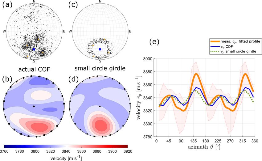
S. Hellmann et al.: Velocity measurements for COF detection                                                                    3511

ital oscilloscope (LeCroy WaveSurfer 3024). For each mea-           nary images as the fraction of air voxels in the image. The ice
surement, we stacked at least 20 individual waveforms to en-        core consists mainly of ice and air captured in bubbles. Liq-
hance the signal-to-noise ratio. Since the amplifiers caused        uid water was refrozen during storage of the core segments,
delays, we determined the actual zero-time of the entire sys-       and dust and sediment particles can be neglected. Therefore,
tem by a regression through repeated measurements on steel          we classify the images as two-phase systems with air bubbles
cylinders with precisely determined lengths. These calibra-         in ice.
tion measurements were performed at least twice a day under
identical temperature conditions.
   The transducers were screwed in an aluminium tube which          3     Data analysis and results
was held by an aluminium frame with an inner diameter of
                                                                    3.1    Acoustic velocities inferred from COF
90 mm in which the ice core with a variable diameter (aver-
age diameter: 68 ± 0.36 mm) was placed. Due to the thermal          Seven ice core samples, obtained from 2, 22, 33, 45, 52, 65
drilling method, thin water layers refroze along the ice core       and 79 m depth, were analysed. The corresponding COF pat-
surface, which led to a rough and partially concave surface.        terns (presented in Fig. 2a–g) are obtained from a set of ice
This uneven surface and the limited height of the transducer’s      core thin sections from two adjacent ice core segments. They
tip resulted in a poor coupling, and we removed the outer-          exhibit clear multi-maxima patterns in all samples, consisting
most 3 mm thin ice layer (i.e. this meltwater “skin”) by lath-      of four (five for 65 m) significant clusters of c axes. These
ing the sample. The ice core diameter was then determined           clusters always form a “diamond shape” pattern and have
manually for each individual measurement. In addition to the        been found to be typical for temperate ice with branched,
horizontal measurements, vertical measurements were per-            large ice grains. We employed a spherical k-means clustering
formed (average length of the samples: 70.6±1.3 mm). The            algorithm (Nguyen, 2020) to determine the individual clus-
1 MHz source pulse generated signals with wavelengths of            ters of grains and their respective centroids. Ice grains that
≈ 3.8 mm. This resulted in a sample size to wavelength ratio        are not assigned to one of the clusters (small black dots in
of approximately 20. Thus, the wavelength is small enough           Fig. 2a–g) are not considered for the velocity calculation as
to measure an integrated seismic velocity. This velocity can        they mostly appear within fracture traces (particularly in 22
be regarded as the integrated velocity of the individual grain      and 45 m). Further details about the crystal structure are dis-
velocities. Much larger wavelengths may introduce geomet-           cussed in Hellmann et al. (2021).
ric issues such as stationary waves which are not representa-          We calculated the acoustic velocities from the COF pat-
tive of acoustic waves travelling through the glacier and thus      terns of all samples. The resulting velocity distributions
would later inhibit a comparison with in situ data. However,        (Fig. 2h–n) are functions of azimuthal direction and incli-
even with such small wavelengths, some measurements may             nation (i.e. colatitude, 0◦ parallel to vertical core axis). The
be biased by only a few larger grains present in these samples      velocities were calculated on a dense grid for azimuth and
of temperate ice. Therefore, we performed measurements at           inclination angles of the incident seismic wave with 1◦ for
three levels of the ice core samples (denoted as zi , i = 1, 2, 3   both angles to avoid interpolation artefacts. The direction of
in Fig. 1a, offset 1z ≈ 35 mm) and averaged the results. We         the maximum velocity in each sample coincides in general
assume this stacking procedure to be comparable with the            with the centroid of the multi-maxima cluster (Fig. 8a–g).
combination of several thin sections for the COF analysis.          The exact position of the centroid and thus the velocity max-
                                                                    imum depends on the weighting factor that considers the size
2.4   X-ray measurements for air content estimation                 of the individual ice grains. This may lead to a slight off-
                                                                    set between the geometrical midpoint of the diamond-shape
In addition to the ultrasonic measurements, the porosity (i.e.      pattern and this centroid of the multi-maxima pattern. The
the volume of air within the ice) was analysed by X-ray             minimum velocity is found on a small circle with an open-
micro-computer tomography (CT) scans. For the scanning              ing angle of about 45◦ around the centroid. Perpendicular to
and analysis, we followed the same procedures previously            the centroid, another minor velocity maximum along a girdle
adopted for bubbly ice from Dome C (Fourteau et al., 2019).         can be observed. The median value of the pure ice veloc-
The samples placed within the CT scanner had a diameter             ity per sampling depth lies between 3834 and 3840 m s−1 .
of approximately 18 mm and a length of 70 mm resulting in           The anisotropy generally increases with depth (Table 1) and
images with a resolution (voxel size) of (10 µm)3 (Gerling          reaches a maximum value of
et al., 2017). A set of 2–3 regions of interest (ROIs) with a
                                                                    max(vp ) − min(vp )
maximum height of 15 mm each was defined in the vicinity                                   = 2.32 %                               (1)
of the horizontal levels of ultrasonic measurements, which                 max(vp )
were about 35 mm apart. The greyscale images of the ROIs            at 79 m between the global maximum (around vertical direc-
were automatically segmented into binary (ice–air) images           tion) and minimum velocity values (Fig. 2n).
following the method from Hagenmuller et al. (2013). The               The P wave velocity for vertically incident waves (parallel
air volume fraction was subsequently calculated from the bi-        to z axis of the core) increases with depth, especially for the

https://doi.org/10.5194/tc-15-3507-2021                                                   The Cryosphere, 15, 3507–3521, 2021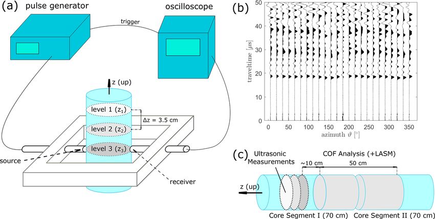
3512                                                                S. Hellmann et al.: Velocity measurements for COF detection

Figure 2. COF patterns and calculated seismic velocities for all seven analysed ice core samples: (a–g) c-axis distribution on a lower
hemisphere Schmidt plot (the core’s vertical axis aligns with the centre of the plot). The grains associated with the individual clusters are
colour-coded. (h–n) Seismic P wave velocities (derived from COF, no air correction) for any azimuthal direction and incident angle plotted
on a lower hemisphere net. They were plotted with the Matlab toolbox MTEX (Mainprice et al., 2011). The black dots symbolise the sets of
angles (ϑ/ϕ) for the ultrasonic measurements.

deepest parts where the cluster is centred around the vertical           per of the two ice core segments that have been used for the
axis (Fig. 3a blue line). The P wave velocities for a colatitude         COF analysis (cf. Fig. 1c). The distance between the upper-
of ϕ = 90◦ (horizontal direction) are shown in Fig. 3b (mean             most COF thin section and the ultrasonic sample is between
value per sample) and Fig. 4. The largest azimuthal variations           5 and 15 cm (with an exception for 65 m with an offset of
appear at 2 m since the c axes of the grains cluster around a            60 cm). For each sample, we carried out three individual hor-
horizontally oriented centroid (ϕc = 88.6◦ ). The maximum                izontal measurements of three different levels (indicated as
horizontal anisotropy is 1.4 %.                                          z1 , z2 , and z3 in Fig. 1a). For the vertical measurements, we
                                                                         obtained one measurement per sample. As there was a half
3.2    Acoustic velocities from ultrasonic experiments                   cylinder of ice from the lowermost depth (79 m) available, we
                                                                         also measured the vertical velocity for this sample. The ultra-
We measured the acoustic velocities on five of the above-                sonic measurements were conducted using different pieces of
mentioned ice core samples. The ice core samples were taken              ice than those used for the COF analysis, and therefore, the
from 2, 22, 33, 45, and 65 m depth and usually from the up-              actual grain size and distribution remain unknown. The posi-

The Cryosphere, 15, 3507–3521, 2021                                                           https://doi.org/10.5194/tc-15-3507-2021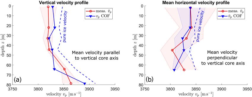
S. Hellmann et al.: Velocity measurements for COF detection                                                                                 3513

Figure 3. Mean values for measured and calculated seismic velocities for (a) vertical, i.e. ϕ = 0◦ , and (b) horizontal, i.e. ϕ = 90◦ , directions
along the ice core. The shaded areas show the standard deviations of the respective measurements. The dashed blue lines show the respective
COF-derived velocities without porosity correction.

Table 1. Mean, minimum, and maximum calculated P wave velocities (i.e. derived from the COF pattern and not from ultrasonic experiments,
without air correction) and degree of anisotropy for each COF sample.

                          Depth (m)                  2         22        33         45         52        65         79
                          v̄p (m s−1 )          3824.5    3824.8     3825.7      3825.9   3824.1     3830.7     3837.9
                          min(vp ) (m s−1 )     3808.3    3804.5     3802.2      3807.8   3800.9     3805.3     3798.7
                          max(vp ) (m s−1 )     3862.8    3864.2     3881.1      3871.6   3863.4     3873.6     3889.0
                          Anisotropy (%)          1.41      1.54       2.03        1.65     1.62       1.76       2.32

tions of the ultrasonic measurements are marked in Fig. 2 by               maximum velocities within the stack of repeated measure-
black dots.                                                                ments for each azimuth are shown as reddish coloured areas.
   In a first step, the recorded traces were shifted to correct               All five samples show a set of two maxima surrounded by
for zero-time t0 , and the P wave arrivals (example shown                  four minima and two local side maxima. For the samples at
in Fig. 1b) were picked. Additionally, the ice core diameter               2, 22, and 65 m depth the positions of the maxima for mea-
for each azimuth was measured, and since the core was not                  sured and COF-derived profiles coincide within a range of a
perfectly round, the diameter varied by a few millimetres.                 few degrees of azimuth (≤ 15◦ ; Fig. 4a, b, e). At 33 m, there
The velocities for each azimuth were calculated using the ice              is a significantly larger azimuthal shift (30◦ ; Fig. 4c), and for
core diameter and the P wave travel time. We measured the                  the sample at 45 m maxima of one profile coincide with a
ice core diameter for each measurement individually, and we                minimum of the other (Fig. 4d). The measured velocity pro-
found no dependence of calculated seismic velocities on the                files show higher amplitudes between maximum and mini-
measured ice core diameters.                                               mum compared to the calculated COF-derived profiles. The
   To ensure data consistency, the reciprocal travel times                 COF-derived profiles are in general rather level with smaller
were compared for quality checks. Rays with opposing az-                   differences between the minima and maxima.
imuths (ϑ and ϑ + 180◦ ) are reciprocal, and the velocity
should be identical. Larger deviations (> 30 m s−1 ) for in-               3.3    Porosity from X-ray tomography
dividual measurements were considered incorrect, and these
measurements were removed from the final dataset (in to-                   The X-ray CT images provide porosity information in the
tal, 7 out of 315 traces). Finally, the reciprocal traces for the          vicinity of the horizontal ultrasonic measurements (sum-
individual horizontal and vertical measurements were com-                  marised in Table 2). The porosity is governed by air bubble
bined, and an average velocity for each azimuth was calcu-                 layers in the ice. These air bubble layers show a preferen-
lated. That is, we only consider an azimuthal range of 0–                  tially horizontal distribution and alternate with air-bubble-
180◦ , and therefore, the horizontal results show a periodicity            free layers along the entire ice core borehole as shown by
of 180◦ . This processing scheme was applied to all five sam-              images of an optical televiewer (OPTV, images not shown).
ples, and the results are summarised in Fig. 4. Minimum and                We calculated individual values for each sample and the
                                                                           average porosity over all five samples (0.682 %). An ad-
                                                                           ditional porosity analysis based on two-dimensional large-

https://doi.org/10.5194/tc-15-3507-2021                                                             The Cryosphere, 15, 3507–3521, 2021
3514 S. Hellmann et al.: Velocity measurements for COF detection
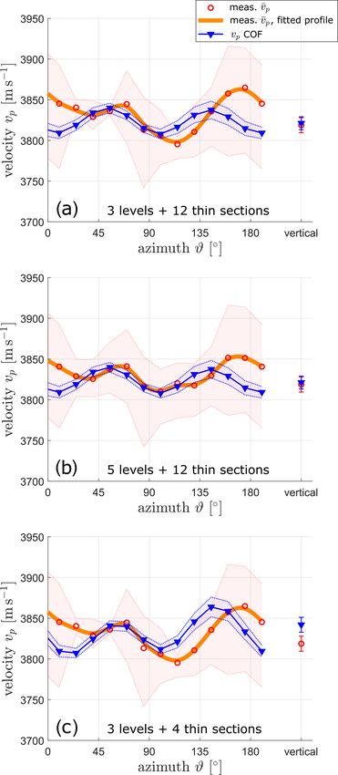
Figure 4. Mean measured seismic velocities from ultrasonic experiments (orange curve and red dots) with maximum and minimum values
(light red areas) for five ultrasonic samples and the corresponding calculated velocities from the COF distribution (blue curve) from Fig. 2
with Voigt and Reuss bounds. These graphs show the horizontal measurements, ϕ = 90◦ . The respective vertical measurement (ϕ = 0◦ ) is
added to each diagram. Depth indicated in upper-right corners.
area scanning macroscope (LASM) images (Binder et al., the LASM images are averaged values obtained from 50 cm
2013; Krischke et al., 2015), obtained during the thin sec- of ice (Fig. 1c).
tion preparation, produced similar results (LASM-derived The individual CT-derived porosity values (Table 2) are
average porosity 0.645 %). In contrast to the porosities from taken into account for the COF-derived vertical velocity
three-dimensional CT measurements, the porosity values de- profiles in Figs. 3 and 4 (blue curves). This correction re-
termined from the two-dimensional LASM images contin- duced the COF-derived velocities by about 30 m s−1 when
uously decrease with increasing depth. This indicates an assuming air-filled spherical bubbles as the second phase
increasingly heterogeneous distribution of air bubbles in (cf. Fig. 3a, dashed magenta line, as an example for un-
deeper parts of the ice since the porosity values derived from corrected values). Since we have a relatively low porosity
(< 1 %) but do not know the exact size and position of the
The Cryosphere, 15, 3507–3521, 2021 https://doi.org/10.5194/tc-15-3507-2021S. Hellmann et al.: Velocity measurements for COF detection 3515
individual air bubbles, we used a correction for spherical surements was approximately 3.8 mm. As a consequence, the
inclusions at a very low volume fraction at which the ef- seismic waves are not just affected by the medium along an
fective elastic moduli can be calculated exactly (Torquato, infinitely thin ray path connecting the source and receiver
2002, p. 499). The CT and LASM images indicate that the but by a finite volume surrounding the ray path. This vol-
majority of air bubbles not associated with grain boundaries ume can be estimated with the first Fresnel volume path (e.g.
(and therefore not pinned to and affected by the boundary Williamson and Worthington, 1993). Assuming a homoge-
pathways) are spherical, do not show any elongation in cer- neous medium including source position S and receiver po-
tain directions, and therefore confirm our assumption. We re- sition R, a point D is considered to be within the first Fresnel
trieved the required bulk and shear moduli of the ice ma- volume when
trix from the corresponding elements of the computed poly- λ
crystal elasticity tensor. With these bulk and shear moduli, SD + DR − l ≤ n , (2)
the CT-derived porosity values, and the mass densities of air 2
(ρ = 1.3163 kg m−3 at an ambient temperature of T = −5◦ ) where l is the direct ray path between source and receiver, n
and ice (ρ = 918 kg m−3 ), we obtained the mean velocities is the order of the Fresnel zone, and λ is the dominant wave-
of such a two-phase material. Finally, the difference between length. The ice grains within this Fresnel volume influence
this mean velocity and the calculated mean velocities of pure the velocity that is derived from the corresponding ultrasonic
ice was subtracted from the individual velocity values. This measurement. To illustrate the situation, we superimposed in
correction was applied to the COF-derived profiles (blue Fig. 5 a Fresnel zone computed from Eq. (2) on one of our
curves) in Figs. 3 and 4. The porosity correction causes a thin sections of temperate ice including large grains. Figure 5
shift of the average velocities (see Fig. 3 dashed vs. solid blue shows that not only the size but also the position of the partic-
lines) but does not affect the shape (i.e. maxima and minima) ular grains may influence how significantly grains of the par-
of the horizontal profiles at the individual depths in Fig. 4. ticular clusters affect the final velocity profile for the ultra-
sonic experiments. If grains of a certain cluster only appear
at the margins of the ice volume (e.g. the dark blue grains),
4 Discussion only a few measurements are affected by these grains, and
thus the overall effect of this cluster is smaller compared to
4.1 Comparing COF-derived velocity and ultrasonic its actual statistical appearance in the ice core volume. The
measurements analysis becomes even more complex when considering the
shape of the grains. As observed in our core data and also in
The results for COF-derived velocities and the ultrasonic ve- earlier studies (e.g. Hooke and Hudleston, 1980; Monz et al.,
locity profiles are compared in Figs. 3 and 4. As presented in 2021) the grains in temperate ice are branched. Furthermore,
Sect. 3.3, the COF-derived velocity profiles were corrected we also observed a clustering of grains with similar orienta-
for the porosity. The vertical velocities (i.e. parallel to the tion. In particular, small grains surround a larger grain, usu-
ice core axis), shown in Fig. 3a, display a relatively good ally called parent grain, as a result of strain-induced grain
match between the two methods. Likewise, the average hor- boundary migration with nucleation of new grains (called
izontal velocity profiles (Fig. 3b) coincide well within the SIBM-N; see Faria et al., 2014). The irregular shape of the
uncertainty ranges. This uncertainty range is defined by the grains and the clustering of grains with similar orientation
standard deviation around the mean value for all azimuths. may lead to differences between the two velocity profiles.
Azimuthal variations in the horizontal measurements are The Fresnel zone is actually a volume (third dimension not
compared in Fig. 4. Only the sample from 22 m depth shows shown in Fig. 5) with the size of a few cubic centimetres.
reasonable matching with respect to the positions and am- The individual measurements are therefore capturing the full
plitudes of the velocity minima and maxima. For all other three-dimensional shape of the grains. Furthermore, the Fres-
depths, there are considerably large differences between nel volume concentrates on a small volume within the sam-
COF-derived and ultrasonic velocities. It is noteworthy that ple. The clustering effect due to SIBM-N leads to an over-
the sample at 22 m depth exhibits a lower porosity (i.e. lower representation of some clusters within these limited volumes.
amount of air bubbles) compared with the remaining sam- Thus, these clusters around a few large grains are dominat-
ples (Table 2), but the air bubble content cannot fully explain ing the measured velocity profile. We have qualitatively anal-
the observed discrepancy between the two velocity profiles ysed this effect and were able to find a combination of two
shown in Fig. 4. These discrepancies could be caused by the or three clusters that reasonably fit into the actual measured
differences in the grain size distribution within the individ- ultrasonic velocity profile. However, several combinations of
ual samples since we did not conduct both measurements on these four clusters led to similar results, and we assume that
exactly the same pieces of ice. the fit might also be a statistical effect. We could not find
Seismic waves have a band-limited frequency content re- a profound physical explanation. Ultrasonic measurements
sulting in a finite range of wavelengths. As indicated in followed by a COF analysis on the same piece of ice are re-
Sect. 2.3, the dominant wavelength for the ultrasonic mea- quired to analyse this further.
https://doi.org/10.5194/tc-15-3507-2021 The Cryosphere, 15, 3507–3521, 20213516 S. Hellmann et al.: Velocity measurements for COF detection
Table 2. Porosity values (%) for each ultrasonic sample (derived from CT measurements) and the corresponding COF thin sections (derived
from LASM scans with a vertical offset of 10–15 cm to CT-samples).
Depth (m) 2 22 33 45 65 Mean
Porosity (CT) (%) 0.63 0.27 0.81 0.35 1.35 0.682
Porosity (LASM) (%) 1.44 0.55 0.68 0.23 0.32 0.645
Figure 6. Number of grains over all clusters in the individual sam-
ples. The mean grain size per sample is noted above. The clusters
are colour-coded according to Fig. 2.
Figure 5. Raw image from fabric analyser, showing a typical grain from the number of grains included in the individual ultra-
distribution found in the temperate ice core. The coverage by ul- sonic measurements, in which a few branched large grains
trasonic measurements (dashed lines) and an example for the first may be quite prominent in the actual measured ice volume
Fresnel zone (homogeneous medium approximation) are superim- (see Fig. 5).
posed: S is the sending transducer, and R is the receiver. The dis- Therefore, the velocities of COF analysis and the ultra-
tance between source and receivers is ≈ 7 cm on average. sonic measurements are expected to be different in the pres-
ence of large grains. Conversely, a good match can be ex-
pected when a large number of small grains is involved. To
In contrast to the ultrasonic measurements, the thin sec- investigate this further, we computed grain size distributions
tions for the COF-derived velocity profiles only provide lim- (Fig. 6) using all thin sections prepared for the COF anal-
ited information in the third dimension. This is even more im- ysis (Hellmann et al., 2021). Clearly, the sample at 22 m
portant for an estimated guess of the size of such branched depth shows the largest number of grains and thus the small-
and large grains. Grains close to the thin section but out of est mean grain size. Considering the previous discussion, it
plane are invisible for the COF-derived velocity profiles. Fur- is therefore not surprising that we observe a relatively good
thermore, a cut through a large branched grain may make match in Fig. 4 for this sample and larger discrepancies for
this grain appear as several small grains, usually called is- the remaining samples.
land grains (see Monz et al., 2021, their Fig. 3). A large As a result of the previous discussion, we also assume
grain is then underrepresented in the COF-derived profiles that a larger amount of ultrasonic measurement levels should
but is more prominent in the Fresnel volume and therefore lead to a better match with the statistically averaged profile
more prominent in the velocities measured by the ultrasonic from the COF analysis. Additional ultrasonic measurements
method. This can be regarded as an out-of-plane effect when are available for the sample of 33 m. These measurements
comparing ultrasonic and COF-derived profiles. To reduce were obtained on the neighbouring core segment just below
this off-plane effect, we have always combined sets of three the analysed COF samples (the original ultrasonic measure-
thin sections perpendicular to each other (see Hellmann et al., ments, shown again in Fig. 7a, were acquired above the COF
2021, their Fig. 4) to obtain the COF-derived profiles. As a samples). When considering the additional measurements,
consequence, the actual number of grains included in the cal- the differences between the mean velocity profiles derived
culations for the COF-derived profiles differs significantly from COF analyses and ultrasonic measurements further de-
The Cryosphere, 15, 3507–3521, 2021 https://doi.org/10.5194/tc-15-3507-2021S. Hellmann et al.: Velocity measurements for COF detection 3517
that provides an integrated COF pattern derived from sev-
eral centimetre-long (up to 50 cm) ice core samples and thus
an averaged velocity. However, both methods are most likely
comparable when the numbers of grains are similar in both
samples. Hence, both methods should be combined, and ul-
trasonic measurements may become a valuable technique to
support the existing method.
4.2 Ambiguities with other COF patterns
In this study, the COF patterns are assumed to be known
a priori, and the ultrasonic results could be correlated with
this known COF. The question that arises is if ultrasonic mea-
surements are a suitable method to determine unambiguously
unknown COF patterns?
To address this question, we consider the sample at 22 m
depth. Its resulting COF and the associated velocity distri-
bution, already shown in Fig. 2b and i, are shown again in
Fig. 8a and b. For this sample, the small grain size pre-
requisite is met, leading to a good match between COF-
derived and ultrasonic velocity profiles (Fig. 4b, shown again
in Fig. 8e without uncertainty ranges). We now compare the
results with a small circle girdle structure (Fig. 8c), which
is a common COF pattern for compressional deformation
in combination with recrystallisation (Wallbrecher, 1986).
Its corresponding velocity distribution is shown in Fig. 8d.
When only considering the horizontal orientations, as mea-
sured with our ultrasonic experimental set-up (marked with
black dots in Fig. 8b and d), the azimuthal velocity varia-
tions of both, the actual “diamond shape” pattern (blue curve
in Fig. 8e) and the small circle girdle (dashed green curve
in Fig. 8e), are compatible with the measured ultrasonic
data (orange curve in Fig. 8e). Obviously, there exist sev-
eral COF structures that explain the ultrasonic data equally
well, thereby leading to ambiguities and uncertainties in in-
terpreting the ultrasonic data. Similar ambiguities can be ob-
served for COF patterns typical for polar ice such as single
maximum vs. girdle fabrics. Adding the additional vertical
measurement parallel to the core axis (black dot in the cen-
Figure 7. Mean measured seismic velocities from ultrasonic experi- tre of Fig. 8b and d) does not remove this ambiguity for the
ments (orange curve and red dots) and the corresponding calculated small-girdle example.
velocities from the COF distribution (blue curve) for the sample at To further reduce this ambiguity, adding additional ultra-
33 m: (a) same as Fig. 4c, (b) with a larger amount of ultrasonic sonic measurements spanning a range of azimuths and incli-
measurements, and (c) with a smaller amount of thin sections con- nations such that the area of the stereoplots would be sam-
sidered for the calculated COF-derived velocity profile.
pled more regularly would be required. With modern point-
contact transducers, it seems to be feasible to implement such
an experimental layout with a reasonable expenditure of time
crease (Fig. 7b). In turn, when considering only a subset of when using a multi-channels recording system.
thin sections (here only the four horizontal thin sections) to These ambiguities show that COF analyses will also be re-
derive the velocity profile, it also converges to the ultrasonic quired in the future, but ultrasonic measurements can support
profile (Fig. 7c). this analysis and bridge the gaps between the discrete COF
To conclude, ultrasonic and COF analyses complement samples. Finally, ultrasonic measurements on ice cores and
each other. The first is a deterministic approach allowing in boreholes provide the link between COF and surface geo-
for a detailed analysis of a particular ice core volume of physical velocities (Bentley, 1972; Gusmeroli et al., 2012;
a few cubic centimetres. The latter is a statistical approach Diez et al., 2014).
https://doi.org/10.5194/tc-15-3507-2021 The Cryosphere, 15, 3507–3521, 20213518 S. Hellmann et al.: Velocity measurements for COF detection
Figure 8. Comparison of different fabric types and their velocity profiles for different inclination angles: (a) lower hemisphere Schmidt plots
for actual multi-maxima fabric for the sample from 22 m and (b) the derived acoustic velocity pattern for (a). (c) Lower hemisphere Schmidt
plots for a modelled small circle girdle fabric and (d) the derived acoustic velocity pattern for (c). The black dots in (b) and (d) symbolise the
horizontal and vertical measurement positions. (e) The velocity profiles for horizontal measurements: orange line – actual measured profile,
blue line – velocity profile of actual COF, and dashed green line – potential velocity profile for a small circle girdle.
5 Future technical improvements improvements require a more comprehensive measurement
device. Such a device could be employed in a processing
Our measurement scheme (Fig. 1a) was built for first at- line (e.g. in polar ice core drilling projects) with existing de-
tempts at investigating the feasibility of ultrasonic measure- vices such as for dielectric profiling (DEP) (Wilhelms et al.,
ments to detect the COF along an ice core and to establish a 1998) before cutting the ice core into sub-samples for dif-
link between COF and cross-borehole or surface seismic ex- ferent analyses. As it also allows for a fast data acquisition,
periments. Although we showed that there are ambiguities, such a device could also be employed for other purposes
such a device provides valuable information and could di- such as detecting the link between two neighbouring ice core
rectly be employed in situ on freshly drilled ice cores. As an segments (i.e. retrieving the actual orientation of the freshly
advantage of an immediate measurement on thermally drilled drilled segment within the glacier).
ice cores, one would avoid the refreezing of meltwater and
thus have a much better coupling of the transducers without
extra work for removing this meltwater “skin”. For mechan- 6 Conclusions
ically drilled cores with a relatively convex shape, the point-
contact transducers are expected to be well coupled. Further- We have performed ultrasonic experiments on ice cores from
more, more than two transducers are recommended to ob- a temperate glacier, and we compared the results with those
tain several inclined measurements as discussed above, and from a well-established COF analysis method. The main ob-
the transducers should further be pressed onto the ice with jectives of this study were (i) to compare the ultrasonic and
a defined constant pressure. A constant pressure is relevant COF-derived seismic velocities and (ii) to check if ultra-
to avoid any pressure melting effects, and it ensures identical sonic measurements have the potential to replace or reduce
coupling conditions. This enhances the comparability of the the labour-intensive and destructive COF analysis. Our main
acoustic signals throughout the entire experiment. findings can be summarised as follows:
In addition, the determination of the exact distance be-
tween source and receiver should be automated. A manual – Ultrasonic and COF-derived seismic velocities are com-
measurement of the distances, as performed in our experi- parable when the grain size of the ice crystals is suffi-
ments, leads to a higher uncertainty in the derived velocities. ciently small. However, this condition is generally not
Moreover it is not feasible with several transducers. These met in temperate ice. As a consequence, we recommend
The Cryosphere, 15, 3507–3521, 2021 https://doi.org/10.5194/tc-15-3507-2021S. Hellmann et al.: Velocity measurements for COF detection 3519
applying this method to cold (e.g. polar) ice cores with Author contributions. This study was initiated and supervised by
small grains. HM, AB, and IW. SH, JK, and IW analysed the ice core microstruc-
ture to obtain the COF and calculate the seismic velocities. SH,
MG, and HL planned and conducted the ultrasonic and CT mea-
– In the presence of large grains, we observe a poor cor- surements. Data processing and calculations were made by SH with
relation between the ultrasonic and COF-derived veloc- support from all co-authors. The paper was written by SH, with
ities. The ultrasonic measurements belong to the deter- comments and suggestions for improvements from all co-authors.
ministic approaches. Each measurement samples the ac-
tual three-dimensional volumes (Fresnel volumes) and
only considers the grains therein. The COF-derived pro- Competing interests. The authors declare that they have no conflict
files provide a statistical mean value of the velocities of interest.
for all thin sections. Therefore, the number of measure-
ment levels of ultrasonic measurements needs to be suf-
ficiently large. This is especially relevant for samples Disclaimer. Publisher’s note: Copernicus Publications remains
from temperate ice cores. neutral with regard to jurisdictional claims in published maps and
institutional affiliations.
– In the presence of a significant porosity (i.e. air bub-
bles), a correction needs to be applied to make ultra- Acknowledgements. The data acquisition for this project has been
sonic and COF-derived velocities comparable. This re- provided by the Paul-Scherrer Institute, Villingen, the Alfred We-
quires the determination of the porosity. In this study, gener Institute Helmholtz Centre for Polar and Marine Research,
we have employed a CT scanner for that purpose. Bremerhaven, and WSL Institute for Snow and Avalanche Research
SLF, Davos. We especially thank Matthias Jaggi, Paul Selvadurai,
and Claudio Madonna for their extensive technical and scientific
– In principle, ultrasonic measurements can be employed support for the ultrasonic measurements and the equipment pro-
for determining COF patterns. However, this requires a vided and Theo Jenk, Margit Schwikowski, and Jan Eichler for their
relatively dense sampling of the ice core, including a support during ice core drilling and processing. We acknowledge
broad range of azimuths and inclination angles. Our ex- Kenichi Matsuoka for the editorial work and the reviewers Valerie
perimental set-up, including only horizontal and vertical Maupin and Sridhar Anandakrishnan for their helpful comments.
measurements, led to ambiguous results.
Financial support. This research has been supported by the
On the basis of our findings, we conclude that ultrasonic Schweizerischer Nationalfonds zur Förderung der Wis-
measurements are not yet an adequate replacement for COF senschaftlichen Forschung (grant nos. 200021_169329/1 and
analysis. However, since the development of ultrasonic trans- 200021_169329/2).
ducers is progressing rapidly, we judge it feasible that ade-
quate experimental layouts of ultrasonic experiments can be
implemented in the foreseeable future. This would offer sub- Review statement. This paper was edited by Kenichi Matsuoka and
stantial benefits since it would reduce the labour-intensive reviewed by Valerie Maupin and Sridhar Anandakrishnan.
COF analysis. Furthermore, the ultrasonic measurements of-
fer the significant advantage of being non-destructive, and
the samples of the generally valuable ice cores would remain
available for other analyses of physical properties. This also
means that the ultrasonic measurements can continuously be References
obtained on freshly drilled cores. Nevertheless, a certain but
Aki, K. and Richards, P. G.: Quantitative Seismology, Quantitative
reduced number of thin sections for a COF analysis can still Seismology, edited by: Aki, K. and Richards, P. G.. University
be used to calibrate the ultrasonic data and to dispose of am- Science Books, 2nd Edn., ISBN 0-935702-96-2, 704pp, 2002.
biguities with direct comparisons of the results of both meth- Alley, R. B.: Fabrics in Polar Ice Sheets: Development and Predic-
ods from the same ice core samples. tion, Science, 240, 493–495, 1988.
Alley, R. B.: Flow-Law Hypotheses for Ice-Sheet Modeling, J.
Glaciol., 38, 245–256, 1992.
Data availability. The ice fabric data and the LASM im- Anandakrishnan, S., Fltzpatrick, J. J., Alley, R. B., Gow, A. J., and
ages are published in the open-access database PANGAEA® Meese, D. A.: Shear-Wave Detection of Asymmetric c-Axis Fab-
(https://doi.org/10.1594/PANGAEA.888518, Hellmann et al., rics in the GISP2 Ice Core, Greenland, J. Glaciol., 40, 491–496,
2018a; https://doi.org/10.1594/PANGAEA.888517, Hellmann https://doi.org/10.3189/S0022143000012363, 1994.
et al., 2018b). The ultrasonic data are available in the open-access Azuma, N.: A Flow Law for Anisotropic Ice and Its Appli-
database ETH Research Collection (https://doi.org/10.3929/ethz-b- cation to Ice Sheets, Earth Planet Sc. Lett., 128, 601–614,
000453859, Hellmann et al., 2020). https://doi.org/10.1016/0012-821X(94)90173-2, 1994.
https://doi.org/10.5194/tc-15-3507-2021 The Cryosphere, 15, 3507–3521, 20213520 S. Hellmann et al.: Velocity measurements for COF detection Azuma, N. and Higashi, A.: Mechanical Properties of Dye 3 Green- Fourteau, K., Martinerie, P., Faïn, X., Schaller, C. F., Tuckwell, R. land Deep Ice Cores, Ann. Glaciol., 5, 1–8, 1984. J., Löwe, H., Arnaud, L., Magand, O., Thomas, E. R., Freitag, Bennett, H. F.: An Investigation into Velocity Anisotropy through J., Mulvaney, R., Schneebeli, M., and Lipenkov, V. Ya.: Multi- Measurements of Ultrasonica Wave Velocities in Snow and Ice tracer study of gas trapping in an East Antarctic ice core, The Cores from Greenland and Antarctica(Investigation into Velocity Cryosphere, 13, 3383–3403, https://doi.org/10.5194/tc-13-3383- Anisotropy through Measurements of Ultrasonic Wave Veloci- 2019, 2019. ties in Snow and Ice Cores from Greenland and Antarctica), PhD Freitag, J., Wilhelms, F., and Kipfstuhl, S.: Microstructure- Thesis, University of Wisconsin-Madison, 1968. Dependent Densification of Polar Firn Derived from Bentley, C. R.: Seismic-Wave Velocities in Anisotropic Ice: A Com- X-Ray Microtomography, J. Glaciol., 50, 243–250, parison of Measured and Calculated Values in and around the https://doi.org/10.3189/172756504781830123, 2004. Deep Drill Hole at Byrd Station, Antarctica, J. Geophys. Res., 77, Gerling, B., Löwe, H., and van Herwijnen, A.: Measuring the Elas- 4406–4420, https://doi.org/10.1029/JB077i023p04406, 1972. tic Modulus of Snow, Geophys. Res. Lett., 44, 11088–11096, Bentley, C. R.: Advances in Geophysical Exploration https://doi.org/10.1002/2017GL075110, 2017. of Ice Sheets and Glaciers, J. Glaciol., 15, 113–135, Gillet-Chaulet, F., Gagliardini, O., Meyssonnier, J., Montag- https://doi.org/10.3189/S0022143000034328, 1975. nat, M., and Castelnau, O.: A User-Friendly Anisotropic Binder, T., Garbe, C. S., Wagenbach, D., Freitag, J., and Kipf- Flow Law for Ice-Sheet Modeling, J. Glaciol., 51, 3–14, stuhl, S.: Extraction and Parametrization of Grain Bound- https://doi.org/10.3189/172756505781829584, 2005. ary Networks in Glacier Ice, Using a Dedicated Method Graham, F. S., Morlighem, M., Warner, R. C., and Trever- of Automatic Image Analysis, J. Microsc., 250, 130–141, row, A.: Implementing an empirical scalar constitutive rela- https://doi.org/10.1111/jmi.12029, 2013. tion for ice with flow-induced polycrystalline anisotropy in Blankenship, D. D. and Bentley, C. R.: The Crystalline Fabric of large-scale ice sheet models, The Cryosphere, 12, 1047–1067, Polar Ice Sheets Inferred from Seismic Anisotropy, IAHS Publ., https://doi.org/10.5194/tc-12-1047-2018, 2018. 170, 17–28, 1987. Gusmeroli, A., Pettit, E. C., Kennedy, J. H., and Ritz, C.: The Crys- Brisbourne, A. M., Martín, C., Smith, A. M., Baird, A. F., Kendall, tal Fabric of Ice from Full-Waveform Borehole Sonic Logging: J. M., and Kingslake, J.: Constraining Recent Ice Flow History at Borehole sonic logging in ice sheets, J. Geophys. Res.-Earth, Korff Ice Rise, West Antarctica, Using Radar and Seismic Mea- 117, F03021, https://doi.org/10.1029/2012JF002343, 2012. surements of Ice Fabric, J. Geophys. Res.-Earth, 124/1, 175–194, Hagenmuller, P., Chambon, G., Lesaffre, B., Flin, F., and https://doi.org/10.1029/2018JF004776, 2019. Naaim, M.: Energy-Based Binary Segmentation of Snow Budd, W. F.: The Development of Crystal Orientation Fabrics in Microtomographic Images, J. Glaciol., 59, 859–873, Moving Ice, Z. Gletscherkd. Glazialgeol., 8, 65–105, 1972. https://doi.org/10.3189/2013JoG13J035, 2013. Budd, W. F. and Jacka, T. H.: A Review of Ice Rheology for Hellmann, S., Kerch, J., Eichler, J., Jansen, D., Weikusat, I., Ice Sheet Modelling, Cold Reg. Sci. Technol., 16, 107–144, Schwikowski, M., Bauder, A., and Maurer, H.: Crystal C-Axes https://doi.org/10.1016/0165-232X(89)90014-1, 1989. Measurements (Fabric Analyser G50) of Ice Core Samples Col- Cuffey, K. M. and Paterson, W. S. B.: The Physics of Glaciers, 4th lected from the Temperate Alpine Ice Core Rhone_2017, PAN- Edn., Elsevier, Amsterdam, 2010. GAEA, https://doi.org/10.1594/PANGAEA.888518, 2018a. Diez, A. and Eisen, O.: Seismic wave propagation in anisotropic Hellmann, S., Kerch, J., Eichler, J., Jansen, D., Weikusat, I., ice – Part 1: Elasticity tensor and derived quantities Schwikowski, M., Bauder, A., and Maurer, H.: Large Area from ice-core properties, The Cryosphere, 9, 367–384, Scan Macroscope Images of Ice Core Samples Collected https://doi.org/10.5194/tc-9-367-2015, 2015. from the Temperate Alpine Ice Core Rhone_2017, PANGAEA, Diez, A., Eisen, O., Weikusat, I., Eichler, J., Hofstede, C., Bohle- https://doi.org/10.1594/PANGAEA.888517, 2018b. ber, P., Bohlen, T., and Polom, U.: Influence of Ice Crystal Hellmann, S., Grab, M., Jaggi, M., Löwe, H., and Bauder, Anisotropy on Seismic Velocity Analysis, Ann. Glaciol., 55, 97– A.: Acoustic Ultrasound Measurements on Ice Core Samples 106, https://doi.org/10.3189/2014AoG67A002, 2014. from Rhonegletscher, ETH Zurich, https://doi.org/10.3929/ethz- Diez, A., Eisen, O., Hofstede, C., Lambrecht, A., Mayer, C., b-000453859, 2020. Miller, H., Steinhage, D., Binder, T., and Weikusat, I.: Seismic Hellmann, S., Kerch, J., Weikusat, I., Bauder, A., Grab, M., Jou- wave propagation in anisotropic ice – Part 2: Effects of crys- vet, G., Schwikowski, M., and Maurer, H.: Crystallographic tal anisotropy in geophysical data, The Cryosphere, 9, 385–398, analysis of temperate ice on Rhonegletscher, Swiss Alps, https://doi.org/10.5194/tc-9-385-2015, 2015. The Cryosphere, 15, 677–694, https://doi.org/10.5194/tc-15- Drews, R., Eisen, O., Steinhage, D., Weikusat, I., Kipfstuhl, 677-2021, 2021. S., and Wilhelms, F.: Potential Mechanisms for Anisotropy Hill, R.: The Elastic Behaviour of a Crystalline Aggregate, in Ice-Penetrating Radar Data, J. Glaciol., 58, 613–624, Proc. Phys. Soc. A, 65, 349–354, https://doi.org/10.1088/0370- https://doi.org/10.3189/2012JoG11J114, 2012. 1298/65/5/307, 1952. Eichler, J.: C-Axis Analysis of the NEEM Ice Core – An Approach Hooke, R. L. and Hudleston, P. J.: Ice Fabrics in a Vertical Based on Digital Image Processing, Diploma Thesis, Freie Uni- Flow Plane, Barnes Ice Cap, Canada, J. Glaciol., 25, 195–214, versität Berlin, 2013. https://doi.org/10.3189/S0022143000010443, 1980. Faria, S. H., Weikusat, I., and Azuma, N.: The Microstructure of Jordan, T. M., Schroeder, D. M., Castelletti, D., Li, J., and Dall, Polar Ice. Part II: State of the Art, J. Struct. Geol., 61, 21–49, J.: A Polarimetric Coherence Method to Determine Ice Crys- https://doi.org/10.1016/j.jsg.2013.11.003, 2014. tal Orientation Fabric From Radar Sounding: Application to the The Cryosphere, 15, 3507–3521, 2021 https://doi.org/10.5194/tc-15-3507-2021
You can also read