Southern Ocean Biogeochemical Argo detect under-ice phytoplankton growth before sea ice retreat
←
→
Page content transcription
If your browser does not render page correctly, please read the page content below
Biogeosciences, 18, 25–38, 2021
https://doi.org/10.5194/bg-18-25-2021
© Author(s) 2021. This work is distributed under
the Creative Commons Attribution 4.0 License.

Southern Ocean Biogeochemical Argo detect under-ice
phytoplankton growth before sea ice retreat
Mark Hague1 and Marcello Vichi1,2
1 Department   of Oceanography, University of Cape Town, Cape Town, 7700, South Africa
2 Marine   Research Institute, University of Cape Town, Cape Town, 7700, South Africa

Correspondence: Mark Hague (mark.hague@alumni.uct.ac.za)

Received: 6 July 2020 – Discussion started: 17 July 2020
Revised: 10 November 2020 – Accepted: 12 November 2020 – Published: 4 January 2021

Abstract. The seasonality of sea ice in the Southern Ocean        1   Introduction
has profound effects on the life cycle (phenology) of phyto-
plankton residing under the ice. The current literature inves-
tigating this relationship is primarily based on remote sens-     The annual advance and retreat of Antarctic sea ice is the
ing, which often lacks data for half of the year or more.         largest seasonal event on Earth, covering some 15 mil-
One prominent hypothesis holds that, following ice retreat        lion km2 (Massom and Stammerjohn, 2010). Such consider-
in spring, buoyant meltwaters enhance available irradiance,       able seasonal changes have profound effects on the life cycle
triggering a bloom which follows the ice edge. However,           (phenology) of phytoplankton residing under the ice (Sallée
an analysis of Biogeochemical Argo (BGC-Argo) data sam-           et al., 2015; Ardyna et al., 2017; Hague and Vichi, 2018).
pling under Antarctic sea ice suggests that this is not nec-      However, the exact character of such effects is currently un-
essarily the case. Rather than precipitating rapid accumula-      known, primarily because studies investigating phenology in
tion, we show that meltwaters enhance growth in an already        these regions have relied on satellite data, which can contain
highly active phytoplankton population. Blooms observed in        missing data for half of the year or more (Cole et al., 2012;
the wake of the receding ice edge can then be understood          Racault et al., 2012). In particular, the winter and early spring
as the emergence of a growth process that started earlier un-     periods are not taken into account, despite the important role
der sea ice. Indeed, we estimate that growth initiation occurs,   they play in both the overall phenology and subsequent sum-
on average, 4–5 weeks before ice retreat, typically starting      mer production (Llort et al., 2015; Ardyna et al., 2017; Boyce
in August and September. Novel techniques using on-board          et al., 2017).
data to detect the timing of ice melt were used. Furthermore,        Here we present the first-ever comprehensive characteriza-
such growth is shown to occur under conditions of substantial     tion of under-ice phenology for this period. This is achieved
ice cover (> 90 % satellite ice concentration) and deep mixed     by leveraging under-ice data collected by Argo profiling
layers (> 100 m), conditions previously thought to be inim-       floats equipped with a suite of biogeochemical sensors, de-
ical to growth. This led to the development of several box        ployed as part of the Southern Ocean Carbon and Cli-
model experiments (with varying vertical depth) in which we       mate Observations and Modeling (SOCCOM) project (https:
sought to investigate the mechanisms responsible for such         //soccom.princeton.edu/, last access: 1 February 2019). Of
early growth. The results of these experiments suggest that a     primary interest to us here is the mechanisms controlling the
combination of higher light transfer (penetration) through sea    timing of phytoplankton growth initiation in the unique en-
ice cover and extreme low light adaptation by phytoplankton       vironment of the seasonal sea ice zone (SSIZ, defined as the
can account for the observed phenology.                           ocean region seasonally covered by sea ice). A dominant idea
                                                                  in the literature with regards to such mechanisms holds that,
                                                                  following ice retreat in spring, buoyant meltwaters tend to en-
                                                                  hance irradiance levels by rapidly shoaling the mixed layer.
                                                                  This alleviation of light limitation (coupled perhaps with nu-

Published by Copernicus Publications on behalf of the European Geosciences Union.
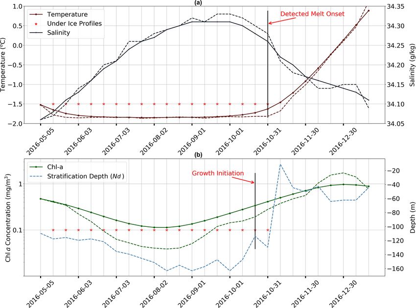
26                                                                  M. Hague and M. Vichi: Under-ice phytoplankton growth

trient input) is then used to explain why blooms are often          different, motivating special attention to this unique environ-
observed in the wake of the receding ice edge (Smith and            ment.
Nelson, 1985; Smith and Comiso, 2008; Briggs et al., 2017;
Sokolov, 2008). The implication here is then that, prior to the
release of meltwaters, growth rates remain low, only increas-
ing substantially in response to melting. Hence, a prediction       2     Methods
of the hypothesis (which we may term the meltwater hypoth-
esis) is that the timing of melting should precede the tim-         The work presented here employs several novel techniques
ing of rapid growth. This is a somewhat subtle point, since         for detecting the timing of phenological events in the sea-
the relevance of meltwaters is usually brought up to explain        sonally ice-covered Southern Ocean. In particular, the use
the presence of blooms, and so is often not explicitly linked       of profiling float data to detect both the timing of melt and
to phenology (e.g. Taylor et al., 2013; Uchida et al., 2019).       growth initiation avoids several of the shortcomings inher-
Nevertheless, the hypothesis implicitly assumes that phenol-        ent to satellite and ship-based studies which characterize the
ogy is strongly affected by the release of meltwater.               present literature on under-ice phenology. First, if in situ data
   However, there is increasing evidence that this is not nec-      are used, they are limited in space and time and are usu-
essarily the case. In an early study, Smetacek et al. (1992)        ally compared to satellite products as a consequence. How-
documented an intense bloom under pack ice conditions in            ever, direct comparisons of this kind are often associated with
early spring (before melting) in the Weddell Sea ice shelf          large uncertainties stemming from the coarse spatial resolu-
region. More recently, in the Arctic, a similarly intense phy-      tion of satellite products and differences in the measurement
toplankton bloom was observed in the Chukchi Sea under              techniques used to produce in situ and satellite data. By using
complete ice cover ranging from 0.8 to 1.3 m thick Arrigo           a consistent observing platform, we largely overcome these
et al. (2012). Although this bloom was observed in sum-             issues, while still achieving good spatial and temporal cover-
mer, Assmy et al. (2017) have recently shown that under-            age at seasonal timescales (see Sect. 3.1). Another clear ad-
ice blooms may develop even earlier in the Arctic due to            vantage of the SOCCOM data set is the availability of depth
the presence of leads in spring. In the Southern Ocean, ev-         information, allowing us to simultaneously compare the sea-
idence is emerging of earlier-than-expected growth in the           sonal evolution of temperature, salinity and chlorophyll a
deep mixed layers within the SSIZ (Uchida et al., 2019;             (Chl a) in the water column and also compare this to diag-
Prend et al., 2019). The important feature of these stud-           nostics such as the mixed layer depth (MLD). Unfortunately,
ies for the present discussion is that high growth rates have       floats analysed in this study are not equipped to measure pho-
been observed prior to melting and under complete (or near-         tosynthetically active radiation (PAR) under ice.
complete) ice cover. However, the present literature has left          We now move on to a more detailed discussion of the
several issues related to under-ice phenology unresolved.           methodology used to detect meltwater release and growth
   First, studies focus almost exclusively on spring and sum-       initiation. Following this, we will describe the biogeochem-
mer and, hence, miss any potential growth occurring in win-         ical model experiments used to investigate the drivers of
ter. Indeed, it is assumed that such growth is negligible even      under-ice growth.
though this has not been explicitly shown. Second, much at-
tention is paid to regions of high biomass (i.e. blooms) and        2.1    Data sources
their associated environmental conditions. Although these re-
gions are no doubt of great interest, their study does not nec-     Float data used in this study are made available by the SOC-
essarily contribute to an understanding of the mechanisms           COM project and can be downloaded through their web-
controlling phenology in general. This is especially true in        site (https://soccompu.princeton.edu/www/index.html, last
the Southern Ocean, where large spatial variability is com-         access: 1 February 2019). Analysis was done on data from
mon (Thomalla et al., 2011). Third, the bulk of the present         2014–2019, making use of Chl a, pressure, temperature,
literature is based on studies of Arctic under-ice phenology.       salinity and position data available at a 10 d frequency. Satel-
Antarctic sea ice is distinct in that it is generally thinner and   lite sea ice concentration for the period January 2015 to
more dynamic and has much more snow year round that does            April 2019 is taken from the NOAA and National Snow and
not form melt ponds (Vancoppenolle et al., 2013). Conse-            Ice Data Center (NSIDC) Climate Data Record (version 3),
quently, the presence of marginal ice zone (MIZ) conditions         which makes use of two passive microwave radiometers,
is also much more prevalent in the Southern Ocean. Note that        namely the Special Sensor Microwave Imager (SSM/I) and
we would define the MIZ here by dynamical considerations            the Special Sensor Microwave Imager/Sounder (SSMIS).
such as wave propagation (i.e. the MIZ may be defined as            The data are downloaded at a daily resolution on the NSIDC
the region where wave attenuation is below a given thresh-          polar stereographic grid with 25 × 25 km grid cells. Finally,
old) and not a satellite ice concentration threshold (for ex-       incident solar radiation at sea level, used to force the model
ample, see Squire, 2007; Meylan et al., 2014). This means           simulations, is taken from the European Centre for Medium-
that seasonal variations in light and nutrients are likely very     Range Weather Forecasts (ECMWF) ERA-Interim reanalysis

Biogeosciences, 18, 25–38, 2021                                                           https://doi.org/10.5194/bg-18-25-2021
M. Hague and M. Vichi: Under-ice phytoplankton growth 27
melting has occurred and attempt to surface when ice is still
present overhead.
While the fact that winter profiles generally only sample
up to ∼ 20 m may seem unimportant, it actually has signifi-
cant bearing on the under-ice detection algorithm used in this
study. This is because, within the upper 20 m in winter, wa-
ter is generally above its freezing point (if salinity is taken
into account). Therefore, in order to delineate under ice from
open ocean profiles, one has to assume some degree of cool-
ing from the last measurement in the profile to the surface.
Since the realized degree of cooling over this winter surface
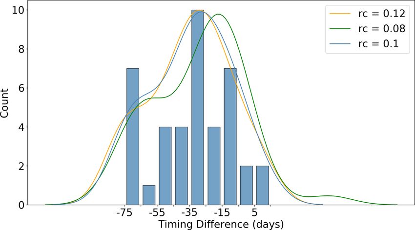
layer cannot be observed, we tested several values (the corre-
Figure 1. Distribution of great circle distances of under-ice pro- sponding effect they had on a key result of the paper is shown
files to the estimated satellite sea ice edge (latitude of 15 % sea ice in Fig. 5). The orange and green curves in Fig. 5 depict the
concentration contour). Negative values indicate that the profile is change in the probability density function when increasing
poleward of the ice edge. and decreasing the cooling threshold (rc) by 20 %, respec-
tively (the details of what is depicted in the figure is discussed
below in the “Growth initiation” subsection). The blue curve
data set. The data resolution is daily (the mean of the day– and associated histogram depicts the chosen value of 0.1 ◦ C
night cycle) on a 0.75◦ × 0.75◦ regular grid. used in this study (i.e. we assume a decrease of 0.1 ◦ C from
∼ 20 m to the surface). We would note that the essential fea-
tures of the distribution remain unchanged in this sensitivity
2.2 Detection of phenological events test.
In addition to the above testing, two further checks were
Under-ice detection performed to assess the validity of using an assumed rate
of cooling to detect under-ice profiles. The first approach is
The first step in our investigation of under-ice phenology shown in Fig. 1, which plots the distribution of distances of
was to determine which profiles could be classified as sam- the under-ice profiles to the satellite ice edge. Here the ice
pling under ice. Since many of the floats deployed in the edge is defined by the 15 % sea ice concentration contour,
SOCCOM project are intended to sample under ice, an ice following previous satellite-based studies (e.g. Stroeve et al.,
avoidance algorithm is utilized on board. The ice-sensing al- 2016) We found that the vast majority of profiles were lo-
gorithm simply compares the median temperature between cated 100 km or more south of the ice edge, with 13.6 % be-
∼ 50 and 20 m during ascent to a threshold temperature of ing north of the edge. It is important to point out here that,
−1.78 ◦ C. If the observed value is lower than the threshold, while sampling under ice, floats do not communicate their
it is assumed that sea ice is present overhead. The float then location since they are prevented from surfacing. A simple
terminates its ascent, stores the profile data and returns to its linear interpolation is used to estimate the location of the
parking depth (Riser et al., 2018). under-ice profiles (based on the relative time stamp differ-
Since the freezing point of sea water depends both on ence), with an approximate maximum error of 100 km, as
temperature and salinity, we chose to include near-surface reported by Riser et al. (2018). It is precisely because of
salinity measurements in our revised under-ice detection al- this uncertainty that we chose to use on-board data to de-
gorithm. That is, for each profile, the freezing temperature, tect under-ice profiles (and to detect melting) as opposed to
based on the salinity closest to the surface, is computed and flagging profiles as being under ice based on their relative
compared to the temperature measured at the same depth. It position to the satellite ice edge. The distribution shown in
is important to note that the depth of these near-surface mea- Fig. 1 is included to illustrate that there is a broad agreement
surements will vary from ∼ 20–25 m in winter to ∼ 0–5 m in between the two methods, although the use of on-board data
summer. This is because of the on-board ice avoidance algo- should be more accurate given the uncertainty of the float
rithm described above; in winter the temperature threshold location.
is generally exceeded, so sampling ceases ∼ 20 m from the The second approach used to assess the under-ice detec-
surface, while in other months this condition is generally not tion method involved visual inspection of the time series of
met, so floats are able to sample much closer to the surface. the mean mixed layer temperature and salinity, like those
Therefore, since the on-board ice avoidance algorithm is in- shown in Fig. 2a (a discussion of how MLD is defined is
tentionally conservative, it may assume there is ice present given below under the “Melt onset detection” subsection).
when in fact melting has already occurred (or when the float This consisted of comparing the timing of the transition from
has moved out of an ice-covered region). Conversely, the under ice to open ocean (depicted by the black vertical line
ice avoidance algorithm may also incorrectly determine that in Fig. 2a) with the associated changes in temperature and
https://doi.org/10.5194/bg-18-25-2021 Biogeosciences, 18, 25–38, 2021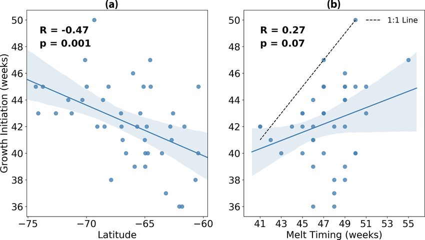
28                                                                  M. Hague and M. Vichi: Under-ice phytoplankton growth

salinity. Both raw (dashed) and filtered (solid) time series are    open ocean, providing further confidence in the melt detec-
shown, with a first-order, low-pass Butterworth digital filter      tion algorithm. Additional figures, which were used to verify
employed with a cut-off frequency of 0.1 Hz. By inspect-            the algorithm, are provided in the Supplement (Figs. S1–S4)
ing a subset of float sampling under ice, we found a good           and show similar results.
visual agreement between the computed timing of the tran-
sition (black vertical line) and the corresponding tendency         Growth initiation (GI)
of the curves toward freshening and warming of the surface
ocean. The best agreement is achieved by assuming a relative        Our main metric for assessing the relationship between melt-
temperature difference (between the last winter measurement         ing and phenology is termed growth initiation (GI). It is de-
and the surface) 0.1 ◦ C as described above, which is why this      fined here as the point at which the time derivative of mean
value was chosen over other candidates. A sample of time            mixed-layer Chl a exceeds the median time derivative com-
series for floats other than those shown in Fig. 2a is provided     puted for the growth period in question. These time deriva-
in the Supplement (Figs. S1–S4).                                    tives, here taken as a proxy for growth rates, are only com-
                                                                    puted over the period of positive growth. This period is de-
Melt onset detection                                                termined from a filtered time series of mean mixed layer
                                                                    Chlorophyll a (Chl a) used to remove variability at the 10 d
Once a transition from ice cover to open ocean has been es-         sampling frequency (the actual value of the median is com-
tablished, our algorithm then verifies that these changes are       puted from the raw signal). A first-order, low-pass Butter-
associated with melting. This is done by computing the time         worth digital filter is employed with a cut-off frequency of
derivatives of the surface temperature and salinity at the time     0.1 Hz. An example of the resulting filtered time series is
of transition (data are taken from measurements closest to          shown in Fig. 2b and compared to the original raw signal.
the surface). In order to be classified as a melt event, the        Also shown in the figure, by the black vertical line, is the
temperature derivative must be positive (i.e. increasing tem-       timing of GI for this particular season. The distance between
perature) with a negative salinity derivative that is persistent    the two black vertical lines in Fig. 2a and b then denotes the
for 1 month following transition. An example of a such a            timing difference between melting and GI, as shown in Fig. 5
melt event is shown in Fig. 2a, where salinity (blue lines)         for all float data.
decreases gradually for ∼ 1 month prior to transition, while           Following Racault et al. (2012), early stages of growth are
temperature (red lines) begins to steadily increase after re-       usually quantified using a metric termed bloom initiation,
maining consistently below freezing. At least three consecu-        which is defined as the time at which Chl a concentration
tive under-ice profiles (equivalent to ∼ 1 month since profiles     first exceeds the long-term median plus 5 %. However, this
are at a 10 d frequency) are needed to detect a melt event.         method is unsuitable in this study for several reasons. First,
In cases where multiple transitions occur in one season, the        our time series are, at most, 4 years long, and on average
transition with the strongest signal (i.e. steepest time deriva-    only 2 years long, precluding an estimation of any long-term
tive) of warming and freshening is chosen. This enables us to       threshold value. Second, our focus is on the conditions which
filter out transitions which occur as a result of advection or      trigger growth, not necessarily a bloom, which again implies
high-frequency warming associated with synoptic variability.        that a comparison to some longer term value must be made.
    Apart from the three criteria discussed above (transition       Finally, we believe a metric based on growth rates (as op-
from under ice to open ocean, positive temperature deriva-          posed to an absolute threshold value) to be more appropri-
tive and negative salinity derivative), an additional inspec-       ate, since it avoids any biases in the median which may be
tion of the time series of stratification depth (our chosen         created by long periods of close-to-zero Chl a concentration
metric for assessing vertical mixing, termed Nd ) was per-          under ice (followed by a rapid increase).
formed. This depth is defined as the point at which the Brunt–
Väisälä frequency reaches its maximum value in the upper            2.3     Model experiments
water column, implying a region of maximum resistance to
mixing (Gill, 1982). Furthermore, this measure of the depth         2.3.1    Model set-up
of the mixed layer has been shown to be more ecologically
relevant in the Southern Ocean than other more traditional          A biogeochemical box model is employed in this study to in-
methods involving density/temperature thresholds (Carvalho          vestigate the drivers of under-ice growth. The model is based
et al., 2017).                                                      on the biogeochemical flux model (BFM) framework, for
    As is discussed in Sect. 1, the release of meltwater tends to   which documentation can be found in Vichi et al. (2015). Our
stratify the surface ocean, so Nd should rapidly decrease fol-      particular configuration is a 0.5D box model in which all the
lowing the detected melt event. In Fig. 2b, we show an exam-        major components of the marine biogeochemical system are
ple of such a time series of Nd (in blue), with profiles flagged    simulated, namely, phytoplankton, zooplankton, organic and
as under ice shown with red stars. One can clearly see that         inorganic matter, nutrients and bacterioplankton. The model
Nd shoals rapidly at the point of transition from under ice to      is termed 0.5D due to the fact that the depth of the box is

Biogeosciences, 18, 25–38, 2021                                                          https://doi.org/10.5194/bg-18-25-2021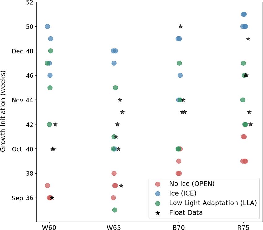
M. Hague and M. Vichi: Under-ice phytoplankton growth                                                                                   29

Figure 2. Time series of key properties illustrating the methodology used for melt and growth detection. (a) Near-surface temperature (dark
red) and salinity (grey) from May to December 2016 in the Ross Sea sector (65◦ S). Red stars indicate profiles flagged as under ice. Solid
lines with markers are filtered time series (higher frequencies have been removed), and dashed lines are raw data. (b) Mean mixed layer
Chlorophyll a (dark green) and mixed layer depth plotted for the same period as in (a). For more information, refer to Sect. 2.2.

able to vary, allowing for the simulation of the effect of ver-         dell Sea study regions (W60 and W65) use an analytical light
tical mixing. In this case, the only effect taken into account          forcing described in Vichi et al. (2015).
is the attenuation of light with increasing mixed layer depth.
   Since our study is process-oriented, we chose to simplify            2.3.2   Experimental design
the model as much as possible while still retaining the major
features of interest. Accordingly, only one phytoplankton (di-          Three core experiments were conducted in four study re-
atoms) and two zooplankton groups (omnivorous mesozoo-                  gions, with each run having a spin-up time of 10 years to
plankton and heterotrophic nanoflagellates) are simulated. In           allow for adjustment to a repeating annual cycle (although
terms of nutrients, phosphate, nitrate and ammonium are in-             in most cases the adjustment took only a few years). In Ta-
cluded, as well as silicate and iron. Initial nutrient condi-           ble 1, we provide an overview of the available float data in
tions were chosen to be representative of the Southern Ocean            each study region. For every complete time series of float ob-
south of ∼ 60◦ S, with non-limiting concentrations of ni-               servations, we performed the set of three core experiments.
trate (31.8 mmol m−3 ), phosphate (2 mmol m−3 ) and silicate            First, two sets of experiments were run to test the effect of
(40 mmol m−3 ; Sarmiento and Gruber, 2006). An initial dis-             sea ice cover on phytoplankton phenology; this included a
solved iron concentration of 0.3 µmol m−3 (Tagliabue et al.,            run with no ice (OPEN) and a run with imposed satellite
2014) was applied to all experiments, which gave the most               sea ice concentration (ICE). A third experiment sought to
realistic magnitude of summer growth when compared to                   test the combined effect that sea ice cover and increased
float data.                                                             low light adaptation (LLA) phytoplankton had on phenol-
   The model is forced daily with solar radiation, satellite sea        ogy. This was achieved by increasing the initial slope of the
ice concentration, float temperature and salinity, as well as           photosynthesis–irradiance curve by a factor of 10, thus en-
mixed layer depth derived from float data (refer to Sect. 2.1           hancing the photosynthetic efficiency at light levels close to
for data sources). Time series of incident PAR and mixed                zero. This value is equivalent to what is commonly used for
layer depth (as estimated by the stratification depth, Nd ) for         sea ice algae (Tedesco et al., 2010).
each study region is provided in Fig. S5. Light available at
the surface is scaled by the sea ice concentration by simply
multiplying the incident radiation by the percentage of open
ocean derived from remote sensing data. Note that the Wed-

https://doi.org/10.5194/bg-18-25-2021                                                                 Biogeosciences, 18, 25–38, 2021
30                                                                  M. Hague and M. Vichi: Under-ice phytoplankton growth

Table 1. Number of floats sampled in each year for the four study   Table 2. Summary of properties of the under-ice BGC-Argo data
regions. This number then corresponds to the number of model runs   set. Note: GI – growth initiation.
done in each region for each of the three core experiments dis-
cussed in the text. Note: W60 – Weddell Sea region at ∼ 60◦ S;        Total floats                            99
W65 = Weddell Sea ∼ 65◦ S; B70 – Bellingshausen/Amundsen Sea          N floats under ice                      20
∼ 70◦ S; R75 – Ross Sea south of 75◦ S.                               N profiles under ice                    753
                                                                      N melt events                           42
            2015   2016   2017   2018                    Float ID     Mean time series length                 27 months
                                                                      Mean timing of GI                       Week 42 (mid-October)
    W60       1       1     1      1                      5904397     Mean timing of melt onset               Week 49 (early December)
    W65       2       2     2      2             5904468, 5904471     Mean Chl a at GI                        0.14 mg m−3
    B70       0       0     2      2    5904859, 5905075, 5905080     Mean peak Chl a                         2.31 mg m−3
    R75       0       0     3      2    5904858, 5904857, 5904860     Mean stratification depth (MLD) at GI   128 m

3     Results
                                                                    (Fig. 4b). Furthermore, almost all events fall below the 1 : 1
The results presented here fall under two general themes.           line in Fig. 4b, revealing that GI tends to precede the release
In the first section, we will test the meltwater hypothesis         of meltwaters.
outlined in Sect. 1, by comparing the timing of the growth             Consequently, in Fig. 5 we plot the distribution of the dif-
initiation (GI) with that of sea ice retreat. Following this,       ference in timing between GI and melting. For the majority
we will present results from a set of simple model experi-          of the observed events, GI occurs well before the release of
ments in an attempt to explain the observed phenology. In           meltwaters (the mean timing difference is 4.5 weeks). Fur-
these experiments, we investigate the role sea ice cover and        thermore, for 35 % of the events, GI is observed more than
phytoplankton low light adaptation play in controlling win-         35 d before melting, with a further 25 % preceding melting
ter/spring growth. By placing the experiments in four distinct      by 25–35 d. Only 10 %, or four events, occur either at the
study regions with different physical conditions, we also uti-      same time as or after the sea ice retreat. In a complementary
lize the spatial and temporal variability available in the float    analysis, we included Chl a data from ∼ 50 m below the es-
data set to derive results of wider regional applicability.         timated mixed layer depth in the calculation of GI. Overall,
                                                                    this tended to shift GI even earlier in the year by diluting
3.1       Observed under-ice growth                                 the summer concentration, although in four cases significant
                                                                    Chl a below the mixed layer enhanced the spring growth rate
Figure 3 plots the approximate mean location of the 42 melt         and thus delayed GI.
events captured in the Biogeochemical Argo (BGC-Argo)                  We would note that our definition of GI (detailed in
data set. From this map it is clear that a fairly broad spa-        Sect. 2.2) is likely to be more conservative than the meth-
tial distribution is achieved, with all the major ocean basins      ods employing a threshold value (i.e. likely to delay growth
sampled. However, the Atlantic and Pacific oceans are better        initiation). In addition, GI was also computed using the mean
represented, with the Weddell, Bellingshausen and Ross seas         mixed layer particulate organic carbon as opposed to Chl a,
having the highest concentration of sampling. Meridional            which resulted in a timing difference distribution similar to
floats sample between approximately 60 and 70◦ S and cover          that shown in Fig. 5 (albeit with a smaller time difference;
the period 2015–2018. Based on this spatial and temporal            see Supplement Fig. S8). In terms of vertical mixing, aver-
distribution, we can expect a large variability in oceano-          age stratification depth (Nd ) at GI is ∼ 128 m, with a standard
graphic conditions. This in turn leads to the large spread ob-      deviation of 51 m. In Fig. S6, we show the value of Nd at GI
served in the timing of GI (from September to January), rep-        for all 42 events and the relationship between Nd and GI. We
resented by the colours of the points in Fig. 3. While there        found that Nd generally ranged between ∼ 75 and ∼ 160 m at
is some indication of the expected progression towards later        the timing of growth initiation, with no correlation between
GI as one moves south (lighter colours), large interannual          Nd and GI. Table 2 highlights some of the salient properties
variability is observed where points are clustered together in      of the data set investigated in this study and summarizes the
space but nevertheless have very different GI values (this dif-     major findings discussed above.
ference is as large as 8 weeks in the Weddell Sea at ∼ 65◦ S).         While the results discussed up to this point incorporate
   In Fig. 4a we show more explicitly the relationship be-          data from all available under-ice floats, in Fig. 6 we focus on
tween growth initiation timing and latitude. Here we find a         three floats which sampled in close proximity to each other
statistically significant correlation (p = 0.001) of −0.47, im-     in the Ross Sea. In the figure, each bold line plots the mean
plying that 22 % of the variance in GI may be explained by          value of five time series which correspond to different melt
variability in latitude alone. Conversely, the relationship be-     events. Events are separated in space and time; in this partic-
tween GI and the timing of meltwater release is insignificant       ular case, 2017 and 2018 were sampled by three floats, which
at the 5 % level (p = 0.07), with a lower correlation of 0.27       resulted in five time series (two each, with one of the floats

Biogeosciences, 18, 25–38, 2021                                                            https://doi.org/10.5194/bg-18-25-2021
M. Hague and M. Vichi: Under-ice phytoplankton growth 31
Figure 3. Approximate locations of melt events identified in the under-ice Biogeochemical Argo (BGC-Argo) data set. The solid black line
represents the mean maximum extent of the 15 % sea ice concentration contour for the period 2015–2018, while dashed lines represent the
interannual variability. The colour of each point represents the timing of the growth initiation (GI) in weeks of the year. Red boxes refer to
study regions discussed in the text.
only sampling in 2017). This allows for a clear comparison sampled in relative proximity north of 75◦ S (region R75).
of the seasonality of Chl a and sea ice, serving as a good Finally, we selected three additional floats which sampled in
example of how phytoplankton are able to sustain growth the Amundsen/Bellingshausen Sea (just north of Pine Island
under near-complete (according to satellite information) ice Bay) around 70◦ S (region B70). This allowed us to compare
cover. Indeed, in this particular case, the average satellite sea experiments run under different forcing conditions (in partic-
ice concentrations were consistently above 90 % until late ular, sea ice concentration, light and mixed layer depth).
November, by which point Chl a has already been steadily Three core experiments were conducted for each region,
increasing for 2–3 months. Examples of other regions can be consisting of first running with no sea ice forcing (OPEN),
found in Fig. S7. then with satellite-derived ice concentration (ICE) and, fi-
nally, with the low light efficiency of phytoplankton en-
3.2 Regional modelling of under-ice growth hanced by a factor of 10 (LLA; sea ice forcing is also kept for
these runs). Within each of the four study regions, this set of
In order to further investigate which factors may drive early experiments is conducted for each year available in the float
growth under ice, we conducted several simplified model ex- data (and in some cases multiple times for the same year if
periments in 4 study regions. The objective here is to deter- more than one float sampled the region; see Table 1). Refer
mine which experiments most closely resemble the observed to Sect. 2.3.1 for more information on the model setup and
seasonality of mixed layer Chl a, thereby inferring which forcing and to Sect. 2.3.2 for the experiment design.
factors may be important in promoting under-ice growth. The results of all experiments are shown in Fig. 7 and are
Each region was chosen based on the spatial distribution of compared to the phenology obtained from float data. This is
melt events shown in Fig. 3. In the Weddell Sea close to 0◦ , done by averaging each of the three core experiments across
two distinct clusters of melt events are seen in Fig. 3 – one each study region to give the mean time series of mixed layer
centred just south of 60◦ S and the other around 65◦ S. For Chl a shown by the red (OPEN), blue (ICE) and green (LLA)
ease of identification, we call these regions W60 and W65, bold curves (the same is done for the corresponding float ob-
respectively. In the Ross Sea, we selected three floats which
https://doi.org/10.5194/bg-18-25-2021 Biogeosciences, 18, 25–38, 202132 M. Hague and M. Vichi: Under-ice phytoplankton growth
Figure 6. Satellite sea ice concentration (SIC) versus Argo float
Chl a for region R75. Shaded regions around each line represent
Figure 4. Timing of growth initiation (GI) plotted against (a) aver- both the spatial and temporal variability present in each data set.
age latitude and (b) timing of sea ice melt for each of the 42 melt That is, each bold line plots the mean value of five time series which
events shown in Fig. 3. Overlain in blue is the linear regression, are each associated with a specific melt event. Events are separated
with the 95 % confidence intervals for 1000 bootstrapped resamples in space and time; in this particular case, 2017 and 2018 were sam-
shaded in light blue. In panel (b), the dashed black line represents pled by three floats (see Table 1), which resulted in five time series
the 1 : 1 line. (two each, with one of the floats only sampling in 2017). The red
star represents the mean value of GI.
By comparing the key phenological features of the time
series shown in Fig. 7, we can examine which of the three
model configurations most closely matches the float time se-
ries. The primary features of interest to us here are timing of
the initial growth (i.e. a switch declining to increasing Chl a
concentrations) and the subsequent rate of growth in spring.
Other features, such as the timing of peak concentration and
the intensity of seasonality (i.e. summer–winter Chl a con-
centration), are not discussed in detail here.
The key finding of the figure is that winter and spring phe-
Figure 5. Distribution of the difference in timing (in days) between nology are most closely captured by LLA experiments in the
growth initiation (GI) and melt onset (for all floats sampling under Ross and Bellingshausen/Amundsen seas (regions R75 and
ice). GI is defined as the point at which the time derivative of the B70, respectively), while in the Weddell Sea (regions W65
mean mixed layer Chl a exceeds the median time derivative (com- and W60) a combination of OPEN and LLA experiments can
puted for the growth period). Negative values in the distribution in- account for the phenology of this period. That is, in the Wed-
dicate that GI has occurred prior to the detected melt onset. Curved dell Sea the timing of the transition from negative to positive
lines represent the probability density functions for several values of derivative in Chl a is better represented by OPEN experi-
the assumed cooling threshold (rc) in the upper ∼ 20 m of the water
ments, while the subsequent rate of growth in spring is more
column. This value represents an assumed decrease in temperature
over the upper ∼ 20 m, which is required to delineate under ice from
closely simulated by LLA experiments (Fig. 7a, b). Indeed,
open ocean profiles (since floats do not sample the upper ∼ 20 m in across all regions the OPEN experiments seem to capture
winter, they do not sample water below the freezing point). Refer to the timing of the minimum Chl a concentration in winter
Sect. 2.2 for a discussion of the methodology used to produce the well but then greatly over estimate the spring growth rate.
figure. In almost all cases, the ICE experiments overly dampened
growth in winter and spring, with the switch from the nega-
tive to positive mixed layer Chl a derivative occurring signif-
servations shown in black). The shading around each of these icantly later than observations. However, in the Weddell Sea
curves in Fig. 7 represents variability across the set of model (W60 and W65), this model configuration suffers least from
runs (or float time series), as was discussed above for Fig. 6. the compressed seasonality particularly evident in the winter
For example, in the case of the B70 region (Fig. 7c), a total of months of other experiments.
four runs were conducted for each experiment (correspond- In Fig. 8 we show the timing of GI for each region and
ing to the four float time series available; see Table 1), and experiment, providing a more quantitative view of the rel-
so the shaded regions show the variability present across four ative changes in phenology (each point in the figure repre-
time series. sents a separate year or location). GI for the model time se-
ries is computed in the same manner as in the float data (see
Biogeosciences, 18, 25–38, 2021 https://doi.org/10.5194/bg-18-25-2021M. Hague and M. Vichi: Under-ice phytoplankton growth 33
Figure 7. Time series of mean mixed layer Chl a for each of the four regions discussed in the text. In each panel, the observed values (black)
are compared to three model experiments; runs with no sea ice are shown in red (OPEN), runs with ice are shown in blue (ICE) and runs
with both ice and enhanced low light efficiency by phytoplankton are plotted in green (LLA). The shaded regions for each curve represent
the spatial and temporal variability present in each data set as in Fig. 6. Note that the time series run from April to April.
Sect. 2.2), although there was no need for filtering. While 2008; Sokolov, 2008; Taylor et al., 2013) relying on satellite
the LLA set of experiments generally performs best at repro- data or models, we were able to thoroughly test this hypoth-
ducing GI, there are notable exceptions in each of the four esis by utilizing a unique in situ data set of under-ice profiles
study regions. In the W60 region, the observed GI occurs from BGC-Argo floats. In particular, we were able to test
between early September and mid-October, with OPEN ex- two predictions of the hypothesis; first, that at least part of
periments having growth too early and LLA experiments too the variability in the timing of growth initiation (GI) may be
late. Moving further south to W65, we see that only LLA explained by the timing of sea ice melt, and second, that GI
is able to capture the observed variability in GI, but that, in should either be synchronous with or occur after the release
some cases, OPEN provides the best fit to the data. Contin- of meltwaters.
uing south and west, both B70 and R75 contain cases where Based on the data analysed here, we do not find evidence
GI is best described by ICE simulations. In the following sec- which convincingly supports either claim. In Figs. 5 and 6,
tion, we will bring together both the observational and mod- we clearly demonstrate that phytoplankton are able to sus-
elling results discussed thus far, thereby shedding light on tain growth long before significant freshening of the surface
the possible mechanisms leading to under-ice growth in the ocean. It is important to reiterate here that GI is based on
Antarctic winter and spring. the rate of growth exceeding the median rate, and so the ten-
dency of GI to precede melting (as illustrated by the timing
differences between these events shown in Fig. 5) suggests
4 Discussion that the rate of growth is already well above average prior
to ice retreat. This explains why GI and melting are not cor-
4.1 Relationship between melting and growth related in time (Fig. 4b); the release of meltwaters does not
appear to relieve light and/or nutrient limitation, and so vari-
The central question of the present study relates to which
ability in melt timing cannot account for variability in GI.
conditions are necessary to trigger phytoplankton growth in
GI is instead correlated more strongly with latitude (Fig. 4a),
the Antarctic SSIZ. As has been outlined in Sect. 1, a popular
suggesting that phytoplankton are responding to changing in-
hypothesis holds that the release of buoyant meltwaters fol-
cident light conditions rather than fresh water fluxes. To be
lowing sea ice retreat shoals the mixed layer, relieving light
clear, the latitudes plotted in Fig. 4a are computed based on
limitation and triggering rapid growth. In contrast to previ-
the approximate location of the float at GI, which in almost
ous studies (e.g. Smith and Nelson, 1985; Smith and Comiso,
https://doi.org/10.5194/bg-18-25-2021 Biogeosciences, 18, 25–38, 202134 M. Hague and M. Vichi: Under-ice phytoplankton growth
nificant compared to the rest of the growth phase. Briggs
et al. (2017) note that nitrate, oxygen and dissolved inorganic
carbon (DIC) change during the ice-covered period are con-
sistent with net respiration; however, the modest phytoplank-
ton standing stock present at GI (which occurs at the end of
the ice-covered period) may not be sufficient to appreciably
reduce nitrate and DIC concentrations and increase oxygen
values (see mean Chl a concentration at GI in Table 2). Thus,
the seemingly contradictory conclusions of our results are
due to differences in which period of the season the analysis
is focussed on, with Briggs et al. (2017) focussing on earlier
periods in the year when the respiration signal is dominant
and the work presented here focussing on the early growth
period when respiration switches to production. In the end,
higher frequency sampling is needed to more precisely de-
termine the timing of net production.
It is also interesting to note that these results can be inter-
preted as supporting the disturbance-recovery hypothesis laid
out by Behrenfeld and Boss (2014). Using this framework,
Figure 8. Timing of GI for each study region (horizontal axis) and Behrenfeld and Boss (2014) and Behrenfeld et al. (2017)
model experiments (coloured points). Corresponding values from
have argued that growth/bloom initiation occurs much earlier
float data are indicated by black stars.
in the year in winter at high latitudes than previously thought,
a very similar conclusion to that is arrived at here. How-
ever, as will be discussed below, the winter growth shown
all cases corresponds to an under-ice condition. Therefore, here does not necessarily require that ecological interactions
the correlation found in Fig. 4 implies that light may be non- be invoked to explain it. Indeed, in our regional box model
limiting under Antarctic sea ice (at least in the conditions experiments (discussed below), we found that zooplankton
sampled by the floats), provided it is late enough in the sea- have a lagged response to diatom growth in early spring
son for there to be sufficient light available at the surface. (see Fig. S9), suggesting that other factors are responsible
Also noteworthy is the extent to which growth occurs prior for the timing of the initial growth. Furthermore, altering the
to melting, with ∼ 60 % of events preceding melting by a zooplankton model parameters (such as lowering the diatom
month or more. As is discussed in Sect. 3.1, our float data set availability) did not lead to a phenology resembling the float
samples in a wide variety of environmental conditions which data. We therefore note that, while the role played by ecolog-
exhibit very different sea ice and vertical mixing regimes. ical interactions is not ruled out here, it can be argued that
This suggests that the results presented here are fairly rep- the observed growth can be accounted for by a revision of
resentative of the SSIZ as a whole, rather than being biased our understanding of the under-ice light environment and the
by a particular region or time period. In summary, we have physiological response by phytoplankton.
shown that prolonged under-ice phytoplankton growth prior
to retreat is typical of the Southern Ocean SSIZ. 4.2 Growth under extreme light limitation
These findings are broadly in agreement with those pre-
sented by Uchida et al. (2019), who analysed the same We now move on to the question of how phytoplankton are
data set and found that early growth initiated in Au- able to sustain growth under such poor ambient light condi-
gust/September in the region south of ∼ 60◦ S. However, the tions. Recall that the average stratification depth at the time
authors do not explicitly investigate growth in relation to the of GI is around 130 m and that satellite data suggest near-
release of meltwaters in the SSIZ and appear to conclude that complete ice cover. Although the timing of GI in October
melting generally initiates growth through the release of iron would allow for ample light in open ocean conditions, pre-
trapped in sea ice and the relief of light limitation. vious studies suggest that light transmittance through typical
Our findings are also complementary to those of Briggs consolidated ice would be just 1 %–5 % of that incident at
et al. (2017), who analysed nine under-ice floats deployed the surface (even with a thin snow layer; Fritsen et al., 2011).
in 2014 and 2015 in the Ross and Weddell seas. Although Two possible explanations for growth under these conditions
the authors concluded that respiration dominated during the are then apparent; one, light is more readily available in ice-
ice-covered period, their Figs. 4 and 6 show that production covered environments than previously thought, and two, phy-
begins before the end of the ice-covered period. Indeed, our toplankton are more adapted to extreme low light than pre-
interest has been the period of initial growth when overall viously thought. Hence, the phenomenon can be accounted
biomass is still generally very low, but growth rates are sig- for by both physical factors (such as sea ice and vertical mix-
Biogeosciences, 18, 25–38, 2021 https://doi.org/10.5194/bg-18-25-2021M. Hague and M. Vichi: Under-ice phytoplankton growth 35 ing conditions which alter light availability) and biological crucial point here is that 100 % sea ice cover (in the winter ones (such as phytoplankton physiology). Both factors are Antarctic sea ice) as seen from satellite does not necessar- likely operating simultaneously. Indeed, the very presence of ily imply a completely consolidated ice surface (Vichi et al., growth indicates light levels above zero, suggesting a revi- 2019). While the ocean may indeed be completely covered, sion of our current understanding of under-ice environments. the ice itself may be unconsolidated, being primarily com- In our regional box model experiments, we explore both posed of pancakes loosely connected by frazil or brash ice. physical and biological factors. The fact that winter and Such a condition is common in the Southern Ocean and is spring phenology is brought closer to observations when low maintained by wind and wave action far from the ice edge. light efficiency is enhanced by an order of magnitude (to a Waves are known to propagate several 100 km into the ice, value typical of sea ice algae) certainly suggests a role for effectively preventing the formation of pack-ice-like condi- phytoplankton adaptation (Fig. 7 – LLA experiments). How- tions (Kohout et al., 2014; Meylan et al., 2014). Wind forc- ever, the interpretation is complicated somewhat by the fact ing is also known to be highly effective in causing ice break- that, under certain conditions, phenology may be best de- up and motion, with intense synoptic events in the Weddell scribed by simulations with no ice (OPEN) or with ice but and eastern Indian oceans occurring frequently (Vichi et al., standard physiology (ICE). 2019; Uotila et al., 2000). Such events, along with interac- For example, in the Weddell Sea (Fig. 7a, b) early growth tions with the westerly wind belt, drive the formation of gaps in August is best captured by OPEN experiments, but subse- within the MIZ and within pack ice. Therefore, the highly quent spring growth rates (October–November) more closely dynamic nature of Antarctic sea ice may lead to a general align with LLA simulations. The inference here would be enhancement of light availability in the underlying ocean. that, in this region, sea ice is unconsolidated and highly per- The presence of even a tiny amount of light may be expected meable to light, allowing growth to initiate as soon as inci- to induce acclimation in primary producers (that are adapted dent radiation is sufficient. This corresponds well with the to low light), thereby explaining why model configurations correlation between GI and latitude shown in Fig. 4a. This which take this into account produce a more realistic phenol- is despite the apparently near 100 % sea ice concentration ogy. suggested by satellite data (see Figs. 6 and S7). Indeed, at these latitudes, we may actually be in the MIZ, which would explain the higher light permeability. Yet, this is not to say 5 Conclusions that sea ice has no effect; later in the season growth rates are slowed by its presence, explaining why LLA experiments This study has characterized under-ice phytoplankton phe- perform better here. These findings generally agree with pre- nology using a unique data set of BGC-Argo profiles, vious studies which point to light (as opposed to dissolved complemented by a set of process-oriented biogeochemical iron) being the primary driver of early spring growth in the model experiments. We have shown that, rather than acting high latitude Southern Ocean (e.g. see Joy-Warren et al., as a trigger as postulated in previous studies, the release of 2019 and citations therein). We would also note that both meltwaters enhances growth in an already highly active phy- silicate and iron are close to their seasonal maximum con- toplankton population. This may explain the decline in phy- centration during late winter/early spring in all our model toplankton stocks observed by Veth et al. (1992) in meltwater experiments (see Fig. S10), thus ruling out nutrient limita- lenses of the northwestern Weddell Sea. That is, the decline tion in all regions. (in a still highly stratified surface ocean) may be accounted Further south in the Bellingshausen and Ross seas, sea ice for by the natural reduction occurring in a bloom that already is expected to be more consolidated in winter and spring, and started prior to the melting. Such unexpected early growth so phenology is better captured by LLA simulations (note (under presumed severe light limitation) may be accounted that the offset in winter time Chl a concentrations seen in for by a combination of low light adaptation by phytoplank- these regions in Fig. 7c and d is likely due to the need to ad- ton and sea ice permeability with respect to light. We argue just the metabolic loss terms for phytoplankton in full dark- that such permeability is related to wind and wave forcing, ness). However, in two cases the timing of GI most closely which together preserve an unconsolidated ice morphology matches ICE experiments (see Fig. 8; regions B70 and R75). that is not captured by current satellite sea ice concentration This may be accounted for by especially thick snow and ice algorithms. layers in those cases, which led to delayed growth. This high- However, our investigation has not been exhaustive of all lights the importance of the particularities of ice morpholog- possible mechanisms leading to under-ice growth. Future re- ical features and their effect on the light environment, some- search directions could include an examination of potential thing which does not seem to be captured by satellite sea ice discrepancies between the timing of shoaling of the mixed concentration. layer and that of active turbulent mixing (e.g. Carranza et al., Thus, it is both the character of ice and snow overhead 2018; Sutherland et al., 2014). An earlier reduction in mixing and the physiological response to severe light limitation that would increase ambient light and help explain the observed may address the question raised at the start of this section. A under-ice growth. Other ecological factors could also be ex- https://doi.org/10.5194/bg-18-25-2021 Biogeosciences, 18, 25–38, 2021
36                                                                      M. Hague and M. Vichi: Under-ice phytoplankton growth

plored, such as potential interactions between pelagic and              Review statement. This paper was edited by Stefano Ciavatta and
sympagic communities, which are known to be highly effi-                reviewed by two anonymous referees.
cient at low light intensities (Tedesco and Vichi, 2014 and
citations therein). Nevertheless, the findings presented here
have important implications for our understanding of how
the biogeochemistry of the region may change in the future.             References
With possible earlier sea ice retreat, and a generally thinner
and more dynamic ice in some regions (including the Arctic),            Ardyna, M., Claustre, H., D’Ortenzio, F., van Dijken, G., Arrigo,
we may expect even earlier growth than reported here, which               K. R., D’Ovidio, F., Gentili, B., and Sallée, J.-B.: Delineating
would likely alter the seasonal air–sea carbon flux and thus              environmental control of phytoplankton biomass and phenology
the biological carbon pump.                                               in the Southern Ocean, Geophys. Res. Lett., 44, 5016–5024,
                                                                          https://doi.org/10.1002/2016gl072428, 2017.
                                                                        Arrigo, K., Perovich, D. K., Pickart, R. S., Brown, Z. W., van
Code availability. The Python code used in this study is available at     Dijken, G. L., Lowry, K. E., Mills, M. M., Palmer, M. A.,
https://github.com/MarkHague/BGC-ARGO-Tools (Hague, 2020).                Balch, W. M., Bahr, F., Bates, N. R., Benitez-Nelson, C.,
Specifically, the routines used to compute growth initiation (GI)         Bowler, B., Brownlee, E., Ehn, J. K., Frey, K. E., Gar-
timing and melt onset timing are provided.                                ley, R., Laney, S. R., Lubelczyk, L., Mathis, J., Matsuoka,
                                                                          A., Mitchell, B. G., Moore, G. W. K., Ortega-Retuerta, E.,
                                                                          Pal, S., Polashenski, C. M., Reynolds, R. A., Schieber, B.,
Supplement. The supplement related to this article is available on-       Sosik, H. M., Stephens, M., and Swift, J. H.: Massive Phy-
line at: https://doi.org/10.5194/bg-18-25-2021-supplement.                toplankton Blooms Under Arctic Sea Ice, Science, 336, 1408,
                                                                          https://doi.org/10.1126/science.1215065, 2012.
                                                                        Assmy, P., Fernández-Méndez, M., Duarte, P., Meyer, A., Randel-
                                                                          hoff, A., Mundy, C. J., Olsen, L. M., Kauko, H. M., Bailey, A.,
Author contributions. MH conducted the float data analysis, per-
                                                                          Chierici, M., Cohen, L., Doulgeris, A. P., Ehn, J. K., Fransson,
formed the model experiments and wrote the paper. MV conceptu-
                                                                          A., Gerland, S., Hop, H., Hudson, S. R., Hughes, N., Itkin, P.,
alized the model experiments and provided valuable input and ex-
                                                                          Johnsen, G., King, J. A., Koch, B. P., Koenig, Z., Kwasniewski,
pertise in all aspects of the presented work.
                                                                          S., Laney, S. R., Nicolaus, M., Pavlov, A. K., Polashenski, C. M.,
                                                                          Provost, C., Rösel, A., Sandbu, M., Spreen, G., Smedsrud, L. H.,
                                                                          Sundfjord, A., Taskjelle, T., Tatarek, A., Wiktor, J., Wagner,
Competing interests. The authors declare that they have no conflict       P. M., Wold, A., Steen, H., and Granskog, M. A.: Leads in Arctic
of interest.                                                              pack ice enable early phytoplankton blooms below snow-covered
                                                                          sea ice, Sci. Rep., 7, 40850, https://doi.org/10.1038/srep40850,
                                                                          2017.
Special issue statement. This article is part of the special issue      Behrenfeld, M. J. and Boss, E. S.: Resurrecting the Ecolog-
“Biogeochemistry in the BGC-Argo era: from process studies to             ical Underpinnings of Ocean Plankton Blooms, Annu. Rev.
ecosystem forecasts (BG/OS inter-journal SI)”. It is a result of the      Mar. Sci., 6, 167–194, https://doi.org/10.1146/annurev-marine-
Ocean Sciences Meeting, San Diego, United States, 16–21 Febru-            052913-021325, 2014.
ary 2020.                                                               Behrenfeld, M. J., Hu, Y., O’Malley, R. T., Boss, E. S., Hostetler,
                                                                          C. A., Siegel, D. A., Sarmiento, J. L., Schulien, J., Hair, J. W., Lu,
                                                                          X., Rodier, S., and Scarino, A. J.: Annual boom–bust cycles of
Acknowledgements. Data were collected and made freely available           polar phytoplankton biomass revealed by space-based lidar, Nat.
by the Southern Ocean Carbon and Climate Observations and Mod-            Geosci., 10, 118–122, https://doi.org/10.1038/ngeo2861, 2017.
eling (SOCCOM) project funded by the National Science Founda-           Boyce, D. G., Petrie, B., Frank, K. T., Worm, B., and Leggett, W. C.:
tion, Division of Polar Programs (grant no. NSF PLR-1425989),             Environmental structuring of marine plankton phenology, Nat.
supplemented by NASA and by the International Argo Program and            Ecol. Evol., 1, 1484–1494, https://doi.org/10.1038/s41559-017-
the NOAA programmes that contribute to it (http://www.argo.ucsd.          0287-3, 2017.
edu; http://argo.jcommops.org; links are external). The Argo Pro-       Briggs, E. M., Martz, T. R., Talley, L. D., Mazloff, M., and John-
gram is part of the Global Ocean Observing System.                        son, K. S.: Physical and Biological Drivers of Biogeochemical
   We acknowledge the use of the BFM model, which is made freely          Tracers Within the Seasonal Sea Ice Zone of the Southern Ocean
available by the BFM System Team (http://www.bfm-community.               From Profiling Floats, J. Geophys. Res.-Ocean., 123, 746–758,
eu, last access: 11 February 2019).                                       https://doi.org/10.1002/2017JC012846, 2017.
                                                                        Carranza, M. M., Gille, S. T., Franks, P. J. S., Johnson, K. S., Pinkel,
                                                                          R., and Girton, J. B.: When Mixed Layers Are Not Mixed. Storm-
Financial support. This research has received funding from the Na-        Driven Mixing and Bio-optical Vertical Gradients in Mixed Lay-
tional Research Foundation through the South African National             ers of the Southern Ocean, J. Geophys. Res.-Ocean., 123, 7264–
Antarctic Programme (SANAP) and the NRF-STINT bilateral col-              7289, https://doi.org/10.1029/2018JC014416, 2018.
laboration programme.                                                   Carvalho, F., Kohut, J., Oliver, M. J., and Schofield, O.:
                                                                          Defining the ecologically relevant mixed-layer depth for

Biogeosciences, 18, 25–38, 2021                                                                 https://doi.org/10.5194/bg-18-25-2021
You can also read