The Growth Contribution of Colonial Indian Railways in Comparative Perspective
←
→
Page content transcription
If your browser does not render page correctly, please read the page content below
The Growth Contribution of Colonial Indian Railways
            in Comparative Perspective∗
          Dan Bogart†         Latika Chaudhary‡            Alfonso Herranz-Loncán§
                                         February 2015

                                             Abstract
          It is widely recognized that railways were one of the most important drivers of
      economic growth in the 19th and 20th century, but it is less recognized that railways
      had a different impact across countries. In this paper, we first estimate the growth
      impact of Indian railways, one of the largest networks in the world circa 1900. Then,
      we show railways made a smaller contribution to income per-capita growth in India
      compared to the most dynamic Latin American economies between 1860 and 1912. The
      smaller contribution in India is related to four factors: (1) the smaller size of railway
      freight revenues in the Indian economy, (2) the higher elasticity of demand for freight
      services, (3) lower wages, and (4) higher fares. Our results suggest large disruptive
      technologies such as railways and other communication technologies can generate huge
      resources savings, but may not have large growth impacts.

         Keywords: Railways, Social Savings, ICT, India, Growth Accounting

         JEL Codes: N7, O47, P52, R4

  ∗
     We thank seminar participants at UC Irvine and Yale’s conference on New Research in South Asian
Economic History. All errors are our own.
   †
     Associate Professor, Department of Economics, UC Irvine, Email:dbogart@uci.edu
   ‡
     Associate Professor, Graduate School of Business and Public Policy, Naval Postgraduate School,
Email:lhartman@nps.edu
   §
     Associate Professor, Department of Economic History and Institutions, University of Barcelona,
Email:alfonso.herranz@ub.edu
1 Introduction
Advances in information and communications technology (ICT) have transformed economies
around the world. Similar to cell phones and the internet of today, railways were the
most important ICT of the 19th century. Soon after the early construction of railways
in Britain, steam powered railways spread from North-West Europe to Asia and Latin
America beginning in the 1830s. In many countries railways were the engine of growth
lowering transport costs, reducing price dispersion, integrating markets, extending frontiers
and increasing incomes. But, the transformative and often disruptive impact of railways
was not uniform across time and space. Some countries experienced a large economic bang,
while in others the effects were more understated.
In this paper, we estimate the growth contribution of colonial Indian railways and com-
pare it to the performance of railways in four large Latin American economies between the
late 19th and early 20th century. The time frame captures the development of the rail net-
work in these countries and ends just before World War 1. India offers a unique perspective
because the existing evidence paints a mixed picture. On the one hand India fell behind
other economies during the height of the ‘railway era’ from 1860 to 1912. India’s per-capita
income increased just 31% between 1870 and 1910 (from $533 to $697), whereas the Latin
American average increased by 110% (from $742 to $1562).1 Many scholars argue British
colonial policies were the root cause of the decline (for example, Bagchi 1982). Such ar-
guments specific to railways point to high fares, high freight rates and the construction of
several unprofitable railways (Hurd 1983, 2007, Sweeney 2011). On the other hand Indian
railways are thought to be a rare success story for the British Raj. Railways transformed
India from many segmented markets separated by high transportation costs to an economy
with local centers linked by rail to each other and the world. According to Donaldson (2012),
railways raised agricultural incomes by 16% in districts with access to the network. And,
Bogart and Chaudhary (2013) find that the growth and level of Indian railways’ total fac-
tor productivity was large compared to both developed and developing economies by 1913.
Comparing India to similar economies in Latin America can help shed light on this puzzle,
and more generally the different effects of ICTs.
We choose Mexico, Argentina, Brazil and Uruguay (LA4) as the comparison set because
like India these were large economies with extensive rail networks by 1912. LA4 accounted
for 65 percent of Latin American GDP, 59 percent of the population and 79 percent of Latin
American railway mileage. With the exception of Brazil, LA4 were among the few Latin
1
The income per-capita data are from Maddison (2001), reported in 1990 purchasing power parity (PPP)
adjusted dollars.
1American countries to build integrated national railway networks. Similar to India, the LA4
economies heavily relied on primary exports in the 19th century. But unlike India, their
railways were mostly private, they were not colonies and had lower population density (and
consequently higher wages) than India.
Our estimation is based on the growth accounting framework, which incorporates the so-
cial savings methodology. Social savings are the classic metric for evaluating the contribution
of railways following seminal work by Fogel (1964) and Fishlow (1966). The social savings
capture the value of lost resources had the quantity of railway traffic been transported at
the prices of pre-railway transport in a benchmark year, say 1912. In a series of influential
articles Crafts (2004a,b) extended social savings to a growth accounting framework. Accord-
ing to the basic growth accounting identity, income per-capita growth can be divided into
increases in physical capital stock per-capita and “crude” total factor productivity growth
(the so-called “Solow residual”). Crafts measured the contribution of railways to each one of
the components by estimating a railway capital term representing the embodiment of rail-
way technology in the capital stock, and a railway TFP term capturing the resource savings
from lower transport costs. As Crafts shows, under competitive assumptions the TFP term
is equivalent to the additional consumer surplus generated by railways, which in turn is the
same as the social savings corrected by the elasticity of demand.
We extend the social savings methodology in several important ways. First, we decom-
pose the savings for freight into two terms: (1) the share of railway freight revenues in GDP
and (2) the ratio of pre-existing freight rates to railway rates. The share term can be called
the “railway penetration effect” as it captures the degree to which individuals and firms used
railway services. The ratio term can be called the “relative productivity effect” as it measures
to what degree railways reduced freight rates relative to the alternative technology. Second,
we decompose the savings from passengers into similar terms, and go further by decompos-
ing the time cost of traveling, which depends on the hourly wage and the average speed of
trains and alternatives. Third, we incorporate the profits of railways, which represent the
part of TFP growth retained by railway companies and not transferred to users via lower
fares. Quantifying the importance of the various components of the social savings provides
an important step in explaining why a communication technology like railways had a large
impact in one economy, and a smaller impact in another.
The main finding is that railways accounted for a large share of Indian GDP per capita
growth, but they made a smaller growth contribution than railways in the most successful
Latin American economies. Our preferred estimates show that Indian railways contributed
0.29 percentage points to annual income per-capita growth from the mid 19th to the early
220th century, larger than Uruguay (0.11%), similar to Brazil (0.31%), but less than Argentina
(0.65%) and Mexico (0.53%). We perform several robustness checks and the same ranking
of India’s growth contribution carries through. One reaches a different conclusion regarding
the contribution of railways as a share of total income per-capita growth. Railways account
for 73% of all income per-capita growth in India, similar to Brazil at 62%. In contrast,
railways account for a smaller share in Argentina (22%), Mexico (24%) and Uruguay (8%).
In Argentina and Mexico the large savings provided by railways appear relatively small
because income per-capita growth rates averaged 2.6% between the late 19th and early 20th
century. India and Brazil were stagnant in the same period with income per-capita growth
rates averaging only 0.5%.
What explains the differences across countries? The decomposition exercise for freight
suggests Indian freight revenues were smaller as a share of GDP than most LA4, which lowers
the social savings. But, pre-existing freight rates were much higher in India compared to
railway rates, which increases the socials savings. We also find that India had a relatively
elastic demand for freight services, and a higher elasticity lowers social savings because
the latter must be adjusted down to estimate the additional consumer surplus. On net
the relatively elastic demand for freight services in India combined with the smaller freight
revenues contributed to lower consumer surplus from railways because these two factors
more than compensate for the difference in freight rates between pre-existing and railway
transport.
For passenger travel, the decomposition shows India had a relatively high penetration
rate. Lower class passenger travel was huge in India by 1913. However, lower wages in India
reduced the time cost of traveling and hence the social savings. Indian railway fares were
also high compared to wages, which further lowered the social savings. Finally, we find that
Indian railways were profitable in 1912 compared to Argentina and Mexico where railways
earned zero or negative profits. Given the ownership structure of Indian railways, the profits
largely went to the colonial Government and to some degree offset tax revenues on Indians.
Our paper contributes to the large literature on the economic impact of railways.2 We
offer a detailed analysis of the social savings from Indian railways before World War I. India
is an important case because it had the largest railway system in the developing world in
this period. Our results also speak to the literature on the Indian economy. In recent
papers, scholars have studied the historical roots of the service sector (Broadberry and
Gupta 2010), and the long-run adverse impact of direct colonial rule (Iyer 2010). We add to
2
This literature began with the classic works by Fogel (1964) and Fishlow (1965). It has continued with
studies by Coatsworth (1981), Summerhill (2000, 2003), Crafts (2004a), Leunig (2006), Herranz-Loncán
(2006, 2011b, 2014), and Donaldson and Hornbeck (2013) among others.
3this growing literature by studying one of the leading sectors of the economy. Our bottom
line is that railways were the most important driver of economic growth in India before 1913.
This is perhaps unsurprising because productivity growth in agriculture, the largest sector
of the Indian economy was stagnant in this period (Broadberry and Gupta 2010). But,
railways also contributed far less to Indian economic growth compared to other countries.
Our decomposition exercises suggest India’s economic structure is one reason. The more
modest penetration of railways suggests that Indian workers and communities did not fully
assimilate into the global economy when railways arrived. India’s low wages were one key
reason because they lowered the time savings of railways. There were also potential policy
mistakes. Consistent with the extraordinary profits earned by Indian railways compared to
LA4, fares and freight rates were high. Given the colonial Government’s regulatory power
on Indian railways, this would be a failure of colonial policy.
Finally, our results contribute to the literature on ICT. Researchers have found a large
growth contribution from ICT in developed and developing countries (Roller and Waverman
2001, Aker and Mbiti 2010). The estimates presented here on railways are consistent with
communications technologies playing a large and important role. That said, our findings
suggest that where railways were not accompanied by other structural changes, they ended
up accounting for an exceedingly large share of a small total per-capita growth rate.
The rest of the paper is organized as follows. Section 2 provides a brief background on
Indian railways. We describe the social savings methodology in Section 3. Section 4 details
the assumptions and calculations of the different components of the growth contribution.
Section 5 puts Indian railways in a comparative perspective and Section 6 concludes.
2 Background on Indian Railways
By most accounts India’s transportation sector was costly and unproductive at the beginning
of the railway era. India had many rives, but they were often not navigable or seasonal as
in the case of the Ganges and the Indus. India had a long coast line, but shipping was
hampered by seasonality and changing winds. In terms of investments in roads and canals,
India was clearly behind Western countries.
Railways changed India’s transport sector dramatically. British mercantile firms were
among the early advocates for railway construction in India (Thorner 1955). They argued
railways would lower transport costs, allow access to raw Indian cotton and open Indian
markets to British manufactured goods. The first passenger line measuring 32 km opened
in 1853. The size of the network grew rapidly in the 1880s and 1890s with track km
4increasing from 15,000 in 1880 to 54,000 in 1913 (Bogart and Chaudhary 2015). Network
expansion continued after 1913 when we end our analysis, but the pace of development
slowed. Although economic motives spurred the initial wave of construction, political and
development concerns became important beginning in the 1870s. Railways were built in
part to mitigate the effects of famines, put down rebellions, and defend the frontier.
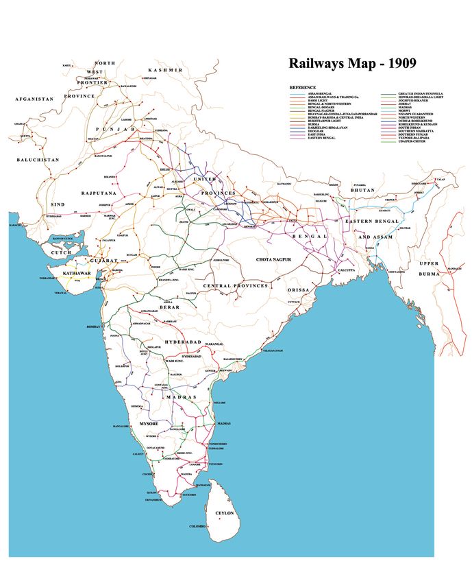
By the early 20th century railways spread to most parts of India as seen in Figure 1
showing the network in 1909 (color coded for each railway system). The first passenger line
connected the port of Bombay to the interior. Similar connections were soon made between
the ports of Calcutta, Madras, and Karachi and their hinterlands. A dense interior network
was constructed between Delhi and Calcutta along the Ganges River, where railways served
long-standing population centers. However, outside of the links with Delhi there were few
interior-to-interior connections. Much of central and southern India was distant from a
railway.
The construction and management of colonial railways involved private British compa-
nies, the colonial Government of India (GOI), and Indian Princely States. In the first phase
up to 1869, private British companies constructed and managed trunk lines under a pub-
lic guarantee. Such guarantees for railway construction were common in the 19th century.
For example, railway companies in Brazil received guarantees of around 7%, large than the
5% in India. In the second phase, the GOI began constructing and managing railways in
the 1870s. The third phase, beginning in the early 1880s, involved hybrid public-private
partnerships between the GOI as majority owner of the line and private companies. In the
fourth phase, starting in 1924, the GOI began taking over railway operations completing
nationalization.3
The structure of the economy matched the flow of goods on the railways. The largest
traffic category was agriculture (see Figure 2).4 It included commodities like grain, oilseeds,
pulses, cotton, tea, and jute. Agriculture, the largest source of Indian exports, was the core
of traffic between the hinterlands and the ports. The second largest traffic category was
minerals, with coal being by far the largest. Coal was shipped internally and was used by
railways distant from mines, and to a lesser extent in manufacturing. Salt, another important
commodity in internal trade, was also part of the mineral category. In comparison, traffic in
manufactured goods was small averaging 5% between 1883 and 1912. Some of these goods
were Indian made, but many were imports.
Several studies have looked at the economic impact of Indian railways. Early work by
3
See Sanyal (1930) for a detailed overview of the regulatory history of Indian railways.
4
The commodity data are from Morris and Dudley (1975, p. 39).
5Hurd (1975) and McAlpin (1974) found less price dispersion and more price convergence
in railway districts compared to non-railway districts and as railways expanded over time.
These studies and those by Studer (2008) suggest a large impact of railways on market
integration. By contrast, Andrabi and Kuehlwein (2010) argue against a large impact.
They regress the price gap for wheat and rice between major Indian cities on an indicator
variable for whether a railway connected the two cities in each year. Unlike the earlier
studies, they focus on changes in price gaps before and after railways link a market pair.
Their estimates imply that railways explain only 20 percent of the overall 60 percent decrease
in price dispersion between the 1860s and 1900s. In a similar vein, Collins (1999) examines
wages and finds limited evidence of convergence during the key decades of railway expansion.
Recently, Donaldson (2012) taking a theoretically grounded and rigorous empirical ap-
proach finds large effects of railways on trade costs and agricultural incomes. He exploits
variation in salt prices, a better proxy for trade costs compared to wheat or rice prices used
in other studies, because salt was produced in one district and transported to others. Using
panel and IV regressions, he finds the arrival of railways increased agricultural incomes by
16% in a district-level analysis. Significantly for our paper, Donaldson estimates the degree
to which railways reduced trade costs relative to carts and boats using differences in salt
prices across districts.
Unlike these studies, we take a macro approach and estimate the impact of Indian rail-
ways by measuring their contribution to the increase in capital stock per-capita and TFP of
the economy. The latter is based on an estimation of the social savings of railways. As is well
known, the social savings compare the freight rates of railways with some alternative, like
bullock carts, and use these figures to measure the income loss from shipping railway traffic
with pre-railway transport technology. The main precedent of our work is Hurd (1983), who
estimated the social savings on Indian freight traffic to be 1.2 billion rupees or 9 percent of
national income in 1900. But, Hurd’s calculation is not detailed. He does not specify the
assumptions, sources or sample. We combine a social savings calculation with the recent
methodology developed by Crafts (2004a) to estimate a precise impact of Indian railways
by 1912 when most of the network was complete. We then compare the Indian experience
to LA4 for which such estimates have already been compiled using the same methodology
(Herranz-Loncán 2014). This exercise puts the Indian experience in a global perspective
and offers a much needed macro view.
63 Methodology
The starting point to measure the growth contribution of a new technology is the usual
Solow expression for increases in labor productivity:
4(Y /L)/(Y /L) = sk 4(K/L)/(K/L) + 4A/A (1)
Where Y is total output, L is the total number of hours worked, K denotes the services
provided by the physical stock, A is “crude” total factor productivity, and sk is the factor
income share of physical capital. This expression has been used in recent research as a basis
for estimating the contribution of general purpose technologies to productivity growth by
distinguishing between different types of capital and different components of TFP growth.
For example, Oliner and Sichel (2002) measure the growth contribution of ICT, both through
disembodied TFP growth and through the embodied capital-deepening effect of investment
in those technologies by transforming expression (1) into:
4(Y /L)/(Y /L) = sko 4(Ko /L)/(Ko /L)+γ(4A/A)o +skict 4(Kict /L)/(Kict /L)+ϕ(4A/A)ict (2)
Where Kict and Ko are the services provided by the capital stock in ICT and in other
sectors, respectively, A is the TFP level in the sector indicated by the subscript (ICT and
other), skict and so are the factor income shares of the capital invested in ICT and other
capital, and ϕ and γ are the shares of ICT and other sectors’ production in total output.
The growth contribution of ICT is the sum of the last two terms of equation (2), which would
approach, respectively, the “capital term” and the “TFP term” of that growth contribution.
In the case of peripheral economies, like India and Latin America, which import new
technologies from core countries where they have been developed for some years, the TFP
term has two components. First, TFP growth within the sector under consideration, and
second, the increase in TFP associated with the substitution of that sector for the previous
technology.
In this context (i.e., railways of peripheral economies), instead of approaching the TFP
term of expression (2) through TFP growth in the railway sector over time, we can esti-
mate TFP by comparing railway transport costs at the end of the period with the cost of
domestic transportation just before the introduction of railways. This would be equivalent
to measuring the social savings of railways as a percentage of GDP:
SS/GDP = (PT R − PRW ) ∗ (QRW /GDP ) (3)
7where PRW and PT R are, respectively, the price of railway and pre-railway transport, and
QRW is the railway transport output in the reference year. The social saving expression (3)
is an upward-biased estimate of the equivalent valuation of consumer surplus provided by
railways, due to the implicit assumption of a price-inelastic transport demand. If the social
savings are corrected for the elasticity of demand and, assuming perfect competition in the
rest of the economy, the elasticity adjusted social savings provides a general equilibrium
measure of the entire direct income gains obtained from transport cost saving (Metzer 1984;
Jara-Díaz 1986). The price dual measure of TFP allows considering such gains as equivalent
to the contribution of railways to TFP growth.5
To see the equivalence between the TFP term and the social savings note that productiv-
ity growth in transport can be written in its dual form as (1/PRW –m/PT R )/(m/PT R ), where
m is the price of inputs in traditional transport relative to railways, whose input prices are
normalized to 1. If one assumes that the prices of factor inputs rise with the general price
level then m/PT R is equivalent to the inverse of the inflation adjusted price of traditional
transport, call it pT R . Rearranging terms we get the following expression for productivity
growth: (pT R /PRW –1). Multiplying the price dual expression for productivity growth by
the revenue share of railway transport in GDP gives an expression for the TFP term as the
social savings: [(PRW ∗ QRW )/GDP ](pT R /PRW –1) or (pT R − PRW ) ∗ (QRW /GDP ).
Our social savings calculation uses the inflation adjusted price of alternative transport
just before the advent of railways (i.e., 1850). We are interested in the contribution of
railways over their predecessor technologies, not the contribution of railways relative to
what alternative transport could have become (as in Fogel 1964). Therefore we exclude
productivity growth in road, river, and coastal transport after railways were adopted. Even
if one thinks that productivity growth in pre-railway transport should be incorporated in the
counter-factual it is likely to be small. We know that productivity growth in British road
and inland water transport required investment in better roads and canals (Aldcroft and
Freeman 1983, Bogart 2005). As of 1850 road and canal investment was not a top priority of
British colonial officials, and it is unclear if that changed in the late 19th century.6 There was
5
However, the potential presence of imperfect competition or scale economies in the transport-using
sectors likely makes the social savings measure a lower bound estimate of the total income gain of railways.
There are other potential TFP spillovers resulting from the commercialization of agriculture, the extension
of finance, and the provision of complimentary public goods like schools. Our view is that spillovers existed
but they were probably second-order compared to the direct resource savings from lower transport costs and
faster speeds, especially in the Indian context where the qualitative evidence suggests there were limited
spillovers to other sectors.
6
Public investment in canal schemes did increase in the late 19th and early 20th century. But these
schemes were about building new canals to harness the water of the Indus river and bring additional areas
under cultivation in Punjab and Sind. There was limited investment in improving existing water transport
8potential for productivity growth in sailing ships, but India had been exposed to European
best practices for more than two centuries. By 1850 they had relatively good sailing ships.
The capital term is usually omitted in the literature on the growth effects of railways.
Most studies make the assumption that the capital invested in railways would have been
allocated to a different sector in the same country with a similar return (Crafts 2004a, p. 7).
It is plausible that, in the absence of the railways, part of the resources invested in railway
construction would have been devoted to improving irrigation. However, due to the foreign
origin of most railway capital in both India and LA4, it is likely that at least part of these
resources would not have been transferred to the Indian and Latin American economies.
Therefore, in a complete counterfactual analysis of the economic impact of railways it is
reasonable to include the growth in the capital stock per-capita associated with the railways
as part of the sector’s growth contribution.
As is shown in expression (2), we estimate the capital term as: skict ∆(Kict /L)/(Kict /L).
This is based on the assumption of constant returns to scale in the production of railway
services and perfect competition both in the railway industry and in the rest of the economy.
This allows us to consider the ratio between net railway revenues and GDP (skict ) as a good
proxy for the output elasticity of capital in the railway industry. These assumptions may
seem strict for a highly-regulated sector such as railways, but the magnitude of the associated
biases is unclear. In the last section we estimate the size of profits in the railway sector and
consider the implications in a comparative context.
4 Estimation for Indian Railways
In this section, we describe the estimation of the TFP term and the capital term in India
between 1860 and 1912. We refer the reader to Herranz-Loncán (2014) for comparable
calculations on Argentina, Mexico, Brazil, and Uruguay (LA4).
4.1 The TFP term: Freight
The TFP term consists of productivity growth in freight and passenger transport, both of
which are measured through the consumer surplus added by railways. The first step in
estimating the surplus from freight is to measure the cost of railway transport in 1912 and
the cost of different transport modes around 1850 before railways were built in India. The
second step is to allocate railway freight traffic in 1912 to the transport modes that would
have been used in the absence of railways. The third step is to calculate the social savings
infrastructure.
9using the cost of freight traffic in 1912 and the cost in the absence of railways. The fourth
step transforms the social savings into additional consumer surplus by correcting for the
elasticity of demand.
As is standard in the literature, we first estimate the cost of railway transport as the
ratio of total freight revenues to total ton miles (the standard measure of freight output in
railways i.e., the number of tons carried one mile). In our case, the ratio is the weighted
average of freight revenues and ton miles of the 17 major railway systems operating in
India.7 The average freight rate was 0.014 rupees per ton km in 1912.8 Next, we estimate
pre-railway freight rates in the regions served by each of the 17 major railway systems. In
these calculations we need to consider the availability of road, river and coastal transport
and their freight rates c.1850 relative to railways in 1912. We begin by estimating the
relative freight rates of each alternative mode.
One strategy would be to use Donaldson’s (2012) calculations. He uses variation in
salt prices across districts and over time to infer relative costs across different modes. His
estimates imply that road transport was 7.88 times more expensive per unit of distance
than railways, and river and coastal were 3.82 and 3.94 times more expensive than railways
respectively. Although his estimates provide a benchmark, they are not well suited for a
social savings calculation for two reasons. First, salt is less bulky to transport as compared
to rice, wheat or other grains. This suggests railways probably charged different freight
rates for salt than other commodities. Hence, salt is unlikely to be representative of the
average charge.9 Second, freight rates for the same commodity differed across railways. A
before-after comparison of salt freight rates within the same railway à la Donaldson does
not account for differences and changes in those differences in freight rates across railway
systems.10
7
These 17 railways jointly accounted for over 90% of the total mileage. Figure 1 shows the rail network
by railway system. Apart from the larger railways, the map also shows the smaller 2 inch gauge railways
that account for less than 10% of mileage and even less of the traffic. We exclude Burma railways in our
calculations because the income data for India excludes Burma as well.
8
Appendix table 1 shows the average rate for the 17 major railway systems and documents the calculation
of the overall weighted average.
9
For individual commodities we can only estimate the freight rates per ton as opposed to per ton km. The
Railway Reports provide data on quantities and revenues by commodity, but they do not give the average
distance hauled. For the most important freight classes in 1901 and 1903, we find salt paid a slightly lower
railway freight rate than grain, oil seeds, and sugar but its freight rate was much less than coal and much
more than cotton. The key question then is whether salt freight rates differed to the same degree on pre-
railway transport. It is difficult to answer this question, but the data on pre-railway freight rates detailed
below suggest that coal paid a similar freight rate to other commodities around 1850.
10
For example, in 1899 the coefficient of variation for grain freight rates per ton mile was 0.22 and the
coefficient of variation for coal freight rates per ton mile was 0.28. On general classes of good the coefficient
of variation was around 0.11.
10On account of these potential problems with using Donaldson’s estimates, we use direct
observations of road, river, and coastal freight rates before railways to estimate social savings.
Derbyshire (1987) is an excellent reference and reports road freight rates in the 1840s and
1850s for north India for pack bullocks, 2-bullock carts, and 4-bullock carts. In rupees per
ton km Derbyshire’s estimates are 0.24, 0.097, and 0.078 for pack bullocks, 2-bullock carts,
and 4-bullock carts respectively. Derbyshire’s figures on road freight rates are consistent with
other sources, especially for carts. Mukherjee (1980) estimates that in Bengal the freight
rate for 2-bullock carts averaged 0.107 rupees per ton km in 1866. Mukherjee also cites
two sources from the mid-19th century which put road freight rates between 3.05 and 4.5
British pence per ton mile. When converted into rupees per ton km, these figures represent
0.079 and 0.116 rupees per ton km. In another source, Ramarao (1998) published the letters
and documents of traders in Bengal, who reported on road freight rates in the mid-1840s.
The average freight rate per ton km in eight reported observations is 0.118 rupees per ton
km. We therefore take Derbyshire’s estimates of road freight rates as being representative
of freight rates by pack bullock, 2-bullock carts, and 4-bullock carts throughout India in the
1840s and 50s.
The next step is to convert Derbyshire’s rates to 1912 prices. Recall that our goal is
to compare pre-railway costs with railway costs in 1912 prices. The most straightforward
inflation factor for this period is the growth in consumer prices. We use the inflation factor
between 1840-59 and 1912 reported in recent work by Allen (2007) and Studer (2008) to
calculate nominal freight rates in 1912.11 These estimates imply larger unit cost differences
from railways compared to Donaldson’s estimates. Pack bullock rates were 35 times the
freight rate of railways and 4-bullock carts were 11 times the railway rate.
We draw on the same sources to estimate freight rates by river transport. Derbyshire
(1987) reports 0.024 rupees per ton km for downstream traffic and 0.039 for upstream. In
other sources, river freight rates are similar. Mukherjee (1980) cites a source which reports
that downstream and upstream rates on the Ganges are 0.03 for downstream and 0.041 for
upstream. Notably the previous water freight rates in Mukherjee include insurance for goods
lost in transit. It was common to take such insurance given the hazards of navigating Indian
rivers. Ramarao (1998 p. 12) cites a source stating that about 20% of the coal shipped by
the Damodar river to Calcutta was typically lost, stolen, or washed away in transit. When
insurance is not included, reported river freight rates are lower. For example, Mukherjee
11
McAlpin’s chapter in the Cambridge Economic History of India (1983) reports price series from 1860
to 1912. These series suggest similar changes in prices as reported in Allen (2007) and Studer (2008) where
the two series overlap in years. We use the more recent price series because they go back to 1840 unlike the
series reported in CEHI.
11cites a source which states that freight rates by unimproved rivers were 0.5 pence per ton
mile, which converts to 0.013 rupees per ton km. There are several downstream river freight
rate observations in Ramarao that do not include insurance and average 0.017 rupees per
ton km.
For the purposes of our social savings calculation we use river rates with insurance.
Indian rivers were hazardous for shipping and without including insurance the costs of water
transport are under-stated. For comparability with road rates we use Derbyshire’s rates for
river transport. One possibility is to average upstream and downstream rates, but it is more
likely that downstream traffic was greater. Moreover, the coal traffic was downstream which
is of special importance to the social savings. Therefore we chose the downstream rate of
0.024 rupees per ton km as our benchmark for water freight rates in the 1840s and 50s.
When adjusted for inflation, the river freight rate in 1912 prices is 0.05 rupees per ton km.
Measured relative to the railway rate in 1912, river transport in India was 3.57 times as
expensive. This figure is quite similar to Donaldson’s relative rate between river and rail.
We have been unable to find direct observations on freight rates for coastal transport in
the source materials. However, there is data on the number of days it took to travel by river
and by sea between various towns. The number of travel days would presumably influence
labor costs and hence a comparison of travel days between river and coastal transport gives
one estimate of the relative freight costs. Deloche (1994) gives figures on travel times in
days at various times of year for coastal regions, and rivers. Using this source we have 16
observations on travel times by river which yield an average of 30.1 km per day. Deloche
also gives 10 observations on travel time for coastal transport, which yield an average of
69.22 km per day. Drawing on this information we assume that the freight rate by coastal
vessel was 42.8% (30.1/69.22) of the freight rate by river which amounts to 0.021 rupees
per ton km in 1912 prices. This is probably an upper bound of the actual rate, since other
differences, such as the larger scale of vessels in coastal than in river transport, may have
reduced freight rates in the former. Table 1 summarizes the information on freight rates.
The next step in the freight social savings calculation is to identify how much rail traffic
would have gone by road, river, or coast in the absence of railways. Our approach assesses
the transport alternatives for each of the 17 major railways systems, and aggregates to
total railway traffic in 1912. The main navigable river systems in colonial India were the
Indus, Ganges and Brahmaputra. The major population centers were generally near rivers
so many railways laid track nearby. For example, much of the East Indian railway followed
the Ganges river valley where population was most dense. The Northwestern railway was
similar in that it followed the more populated Indus river valley. Among the 17 major
12railways systems, seven were close to one of the navigable rivers.12
Proximity to a navigable river gave the possibility to river traffic but there were other
constraints like seasonality and irregularity of water flow. The rivers were too dry for much
of the year and only usable during the monsoon season. According to the railway engineer
George Stephenson, “the great season for the transit of goods to and from northern India is
from July to end of November, the navigation of the rivers during the other seven months of
the year being so tedious and expensive” (Ramarao, p. 46). Observers also remarked that
the water flow of rivers was inconsistent as they depended on the melting of snow in the
Himalayas. In some cases, boats had to be hauled along mud and in other cases, the rivers
were dangerous torrents.
The limitations of river transport meant that there was still a significant amount of
road traffic in areas with navigable rivers. For Bengal there are some specific estimates
of how much traffic went by road and by river prior to railways. Stephenson stated that
for the trade between Calcutta and Burdwan, a town on a tributary of the Ganges, three-
fifths went by river and two-fifths went by road (Ramarao, p. 46). John Bourne’s report
on Indian river navigation in 1849 stated that there were 1.06 million tons carried by the
Ganges river between Calcutta and Mirzapore and 0.106 million tons carried by road (p.
50). Thus according to Bourne just under one-tenth of this trade went by road and just
over nine-tenths went by river. Other records for Bengal support the contention that road
traffic continued in areas with river transport.
Drawing on Stephenson and Bourne one assumption is that for railways near navigable
rivers between 1/10th and 2/5th of the traffic would have gone by road in the absence of
railways. We favor the higher 2/5th assumption because there is a higher risk of over-stating
the amount of counter-factual river traffic for railways near rivers. Many railways lines
diverted from navigable rivers and gained traffic that would have had to travel a significant
distance by road.13 We also present a robustness check using the lower 1/10th assumption
for road traffic.
Coastal trade was widely available in India. Some railway systems in the Indian Peninsula
followed the coast because population was most dense there. An example is the South Indian
12
The railway systems near rivers were the East Indian, Northwestern, Eastern Bengal railway, Oudh and
Rohilkhand, Bengal and Northwestern, and Assam Bengal.
13
The most important example is the coal traffic. For example, by 1870 the Central Indian coal deposits
were served by the East Indian railway, which had some track near the Ganges river but that portion of the
track was at a greater distance from the coal deposits. The coal deposits in Central India are described in
the 1840s as ‘situated beyond reach of the great lines of navigation’. Therefore, based on the geography of
India’s coal deposits it is likely that more than 1/10th of the East Indian’s coal traffic in 1912 would have
had to be shipped by road instead of river.
13railway which had much of its track mileage along the southeastern coast near the city of
Madras. In total 4 of the 17 major railways systems were close to the coastline.14 Like
river transport, coastal transport was also seasonal. The winds generally blew south in the
winter and north in the summer. Thus depending on the direction of trade and time of
year, coastal shipping could be more expensive. Unfortunately it is very difficult to work
out how much traffic would have been shipped by coast and by road in the areas where
the South Indian and similar ‘coastal’ railways operated. For lack of better information we
again assume that three-fifths of railway traffic would have gone by coast and two-fifths by
road. That said, we present a robustness check assuming that only 10 percent of the traffic
went by road similar to Bourne’s assessments for river versus road traffic.
For the remaining railways road transport was the only alternative to railways.15 In
these and all previous railway systems it is important to identify whether wheeled road
traffic was available. Deloche’s (1993, p. 261) exhaustive study of roads and road vehicles
before railways suggests that wheeled traffic was widely available only in northern India,
including Bengal and the Ganges river valley. For the rest of India pack animals were the
typical mode of road transport. Deloche’s argument is supported by John Bourne who
states that camels were the most notable mode of transport in the northwest (pp. 24 and
67). Drawing on these sources, we assume that Derbyshire’s two bullock cart freight rate
applies to the 6 railway systems in northern India and the higher pack bullock freight rate
applies to the rest.16
We summarize our assumption on the share of traffic allocated to road, river, and coastal
transport by railway system in table 2. Pack bullocks account for 35% of traffic, river 36%,
2-bullock carts 20%, and coastal transport 9% in the counter-factual. The allocation of
traffic is important as freight rates differ significantly across modes of freight traffic. Table
3 shows the weighted average freight rate (rupees per ton km) in the counterfactual using
the proportion of traffic allocated to each alternate traffic mode as the weights. We present
estimates using both Donaldson’s costing for pre-railway and railway transport and the
alternative costing we developed using direct observations. Compared to Donaldson, the
direct observations suggest road traffic was more expensive and coastal traffic less. Given
the distribution of traffic to these modes, the counter-factual average freight rate without
14
The railways systems near the coast were Bengal Nagpur, Bhavnagar-Gondal, Madras and South Indian
railway. We did not include any coastal traffic for Bombay, Baroda and Central India because a majority
of their mileage was in-land and only a small proportion was coastal.
15
Railways without rivers or coasts nearby are the Bombay, Baroda and Central India; Great Indian
Peninsula; Rajputana Malwa; Nizam; Udaipur Chitoor; Rohilkhand and Kumaon, and Jodhpor-Bikaneer.
16
The 2-bullock cart rate is assumed for East Indian; Eastern Bengal; Oudh and Rohilkhand; Bengal and
Northwestern; Bengal Nagpur; and Rohilkhand and Kumaon.
14railways turns out to be significantly higher under direct observations. While it is difficult to
say which is more accurate, we prefer using the direct observation freight rate because trade
costs do not necessarily translate into freight costs. Donaldson’s rates are not estimated on
the basis of pre-railway information but from 1870-1930. Moreover, they could be sensitive
to differences in freight rates between salt and other commodities. Finally, the studies on
Latin America also employ the same methods to estimate the freight rate for alternative
transport.
The final step for freight is to estimate the price elasticity of demand and adjust the
consumer surplus accordingly. Without this adjustment the calculation assumes traffic levels
would have been the same without railways even though freight rates, fares, and travel
times are much higher. In other words, it assumes a perfectly inelastic demand. As this
is implausible a correction needs to be made using an estimate for the price elasticity of
demand. The estimates for price elasticity of freight are -0.5 in Mexico (Coatsworth 1981), -
0.6 in Brazil (Summerhill 2000), -0.49 in Argentina (Summerhill 2003), and -0.77 in Uruguay
(Herranz-Loncán 2011b). Most of these estimates come from regressions of railway freight
traffic on freight rates and controls. We apply a similar method for India, but with the
added advantage of using railway-level data from 1880 to 1912 rather than aggregate data
for the whole system, as in other cases. The standard specification for railway demand is
the following where β1 is the estimate for price elasticity:
ln(f reight − ton − miles)it = β1 ∗ ln(real − f reightrate/ton − mile)it + β2 ∗ ln(railway −
miles)it + β3 Y eart + it
Table 4 reports the estimates of the demand equation using the individual railway-level
data. The data series are summarized in Bogart and Chaudhary (2013) and are drawn from
annual Railway Reports published by the Government of India. The first column is the
most parsimonious and suggests a very large price elasticity of -0.95. This decreases to -0.73
when we include railway fixed effects. In specification 3 we control for both railway and year
FE, which allow for more flexibility over a simple trend. The estimate increases to -0.84.
In the final specification, we add railway density (train miles run divided by track miles) as
an additional control resulting in an estimate of -0.66. Since other studies do not include
density in their elasticity estimation, we use the estimate of -0.84 from specification 3 in our
main analysis and present robustness checks using the lower -0.66 estimate.
Equipped with a price elasticity estimate, we use a standard formula for transforming the
social savings into additional consumer surplus.17 Table 5 summarizes the calculations of
17
The ratio between the additional consumer surplus and the social savings is given by [(φ(ε+1) − 1)/((φ −
1) ∗ (1 + ε))], where ε is the price elasticity of transport demand (with negative sign) and φ is the ratio
between counterfactual and railway transport prices; see Fogel (1979, pp. 10-11).
15social savings and the additional consumer surplus in freight. We find large social savings in
freight on the order of 27% of GDP in 1912. After accounting for elasticity, the social savings
translate into 1,216 million rupees of consumer surplus, which is 6% of GDP. Consumer
surplus from freight is lower than the social savings because of the large difference between
the price of alternative transport and railways, and the large price elasticity. If we use the
estimate for the lower elasticity of demand (-0.66), the additional consumer surplus increases
to 8% of GDP.
4.2 The TFP term: Passenger
Like freight, the additional consumer surplus from passenger transport is estimated from
social savings and then corrected for an elastic demand. The social savings in passenger
transport includes money savings from lower fares and time savings from replacing slower
traditional transport. The time savings require data on travel speeds and passengers’ hourly
wages. It also requires an assumption of the share of railway traveling time that would have
been devoted to working. As before we begin with the cost of passenger transport using
railways in 1912 and then proceed to alternatives that would have been used in the absence
of railways.
In India there were four passenger classes for railways. The first class accounted for 0.6%
of passenger traffic in 1912, the second and third together accounted for 5.9% and the fourth
for 93.5%. Naturally fares were highest for the first class at 0.046 rupees per passenger km.
The second and third were similar and averaged 0.016 rupees. The fare for the fourth was
less at 0.007 rupees. The first class was targeted to high ranking British officials. The
second and third classes were meant for upper class Indians and lower class Europeans and
Eurasians (Kerr 2007). The identity of the fourth class is more difficult to establish but it
is likely to have been middle class Indians rather than laborers. As we shall see below the
fare was quite large even relative to skilled wages.
In the literature there is often an assumption that upper class passengers would have
used stagecoach transport in the absence of railways, but all lower class passengers would
have walked. We follow a similar approach for India and assume the first, second, and third
classes would have used wheeled vehicles in the absence of railways. The descriptions of
contemporaries in Bengal published by Ramarao (1998) indicate that wealthy Indians and
British officials travelled in coaches known as daks. Some also travelled in a vehicle known
as a palkeen or palanquin, notable for relying on human instead of animal power. Lastly,
some travelers used the bullock carts transporting goods. Our other assumption is that the
fourth class would have walked in the absence of railways. This is supported by reports of
16the large number of foot travelers in India. For example, on the Annabad bridge during the
year 1837-38 it was noted that there were 435,242 foot travelers compared to 19,869 horses
and 9,314 carts (Ramarao, p. 90).
The pre-railway fares for different travel types are documented for Bengal based on
questionnaires sent to British officials in the 1830s and 40s on passenger travel and are
published in Ramarao (1998). One question asked “What is the expense of the journey by
land from Calcutta to Benares to the natives of various classes; for instance, the wealthy
native traveler of moderate means and lastly to the poor description of pilgrims. . . ?” The
respondent stated that it would be “from 150 to 200 rupees with twelve bearers. In a gharry
will cost 100 rupees and if in a palanquin 125 rupees besides 25 rupees for a banghey to carry
eatables” (Ramarao, p. 91). These fares turn out to yield a passenger per km between 0.15
and 0.29 rupees using a distance of 680km between Calcutta and Benares. They are lower
than other observations for Bengal which quote passenger travel by dak at 0.31 rupees per
passenger km and by palanquin at 0.23 rupees and 0.21 rupees (Ramarao, p. 87, Bourne, p.
51). Drawing on this information we assume that the first class passengers paid the most
expensive fares at 0.31 rupees and that second and third class passengers paid the palanquin
rate at 0.21 rupees. After converting these fares into 1912 prices using the same consumer
price index as for freight, the counterfactual fare is 0.64 rupees per passenger km for first
class and 0.43 for second and third classes. It is noteworthy that dak rates were 14 times
the first class railway fare and palanquin rates were 36 times larger than second and third
class railway fares.
The difference in fares does not apply to the fourth class because we assume they walk in
the absence of railways, which requires no fare. The zero fare assumption for the ‘lower class’
passenger is common in the literature and so we retain it here for comparison with Latin
America. However, it is not entirely satisfactory as walking consumes calories which require
income. Bourne (p. 51) estimates that the expense of traveling by foot in India including
time and subsistence was 0.533 pence per passenger mile or 0.028 rupees per passenger km
in 1912 prices. In an extension we use this figure as the “walking cost” for the fourth class,
even though it conflates time costs which are dealt with separately.
The savings from time require estimates of average travel speeds with and without rail-
ways and the value of passenger’s travel time. The speed of passenger trains in India was
between 27 and 51 km per hour; the average across Indian railway systems weighted by pas-
senger traffic was 36.48 km per hour (Great Britain 1913, p. 445). Prior to trains, speeds
were obviously much slower, but by how much? Ramarao (p. 87) published the Military
Board’s Report on the time occupied between Calcutta and Benares in travel. The Board
17states that it took 18 to 20 days by foot, 15 to 18 days by palkee (palanquin), and 4.5 to 5
days by dak. Assuming a 10 hour travel day and given that the distance between the two
cities is around 680 km, this would imply a travel speed of 3.57 km per hour by foot and
4.12 km per hour by palkee. Another source also implies that the hourly travel speed of
palanquins was 3.86 km per hour (Ramarao p. 87). The Military Board’s reported travel
time for the dak was low compared to others and it is likely that it included night travel.
Assuming a travel day of 20 hours for the dak yields a speed of 7.15 km per hour. Another
source in Ramarao (p. 87) puts the travel speed of daks at 4 miles per hour or 6.44 km per
hour. Drawing on these figures, we assume that prior to railways the travel speed for fourth
class passengers was 3.57 km per hour which is the estimate for walking. The speed for
second and third class was 4.12 km per hour corresponding to the palanquin, and the speed
for first class was 6.44 km per hour corresponding to the dak. By comparison passenger
trains were more than five and half times the speed of the fastest available form of transport
before railways.
For the value of time we assume fourth-class travelers were paid the hourly wage of skilled
workers and that of second and third-class travelers at twice that amount. The hourly wage
of skilled workers is estimated to be 0.059 rupees per hour. It is based on monthly wages in
all regions of India reported in Allen (2007) and assuming 26 days in a month and 10 hours
per day worked on average. Doubling this wage would give second and third class passengers
an hourly wage of 0.118 rupees. First class incomes or wages are known with less certainty,
but assuming they were high ranking British officials they should have received at least
the nominal wage of skilled workers in London. According to Allen’s data London building
craftsman earned 100 grams of silver a day, which translates into 9.27 rupees. Assuming
a 10 hour day would imply that first class passengers earned an hourly wage of at least
0.928 rupees. This figure is not unreasonable as it is around eight times the wage of the
second and third class and 16 times that of the fourth class. Finally, as is customary in the
literature, we assume that only half of the time savings would have been spent working and
earning a wage. Leisure is priced at zero and thus only half the value of the time savings is
included in the social savings.
The final assumption is related to the price elasticity of demand for passenger travel.
In the case of first or upper class transport, the standard assumption is that the demand
elasticity is -1. The justification is that upper class travel contained a luxury element and
that elites would have turned to local activities for entertainment had railways not existed.
By contrast, in the case of the second or lower class, the common assumption is a null
elasticity, which implies that their journeys were mainly made out of necessity (see Herranz-
18Loncán 2014, Leunig 2006). We adopt these assumptions for India and assume a demand
elasticity of -1 for first, second, and third class passenger travel and zero elasticity for fourth
class travel.
Table 6 summarizes the calculations for passenger social savings and the additional
consumer surplus. We show the money and time savings separately and combined. India’s
passenger social savings hinge on whether we include walking costs or not. Without walking
costs the social savings is 3.39% of GDP, which rises to 6.43% of GDP if we include walking
costs. We think it is reasonable to include walking costs because otherwise the social savings
from fourth class travel is essentially zero, which seems implausible. Similar to freight, we
adjust the passenger social savings to consumer surplus using the price elasticity of demand.
The consumer surplus from passenger travel is again lower than the social savings mainly
because of the high price elasticity for second and third class passengers. In total the
additional consumer surplus is 3.51% of GDP. Compared to the freight estimate of 6%,
railway passenger travel generated lower social savings and consumer surplus in India.
4.3 The TFP term: Railway Profits
Railway profits are a part of the resource savings absorbed by producers. Hence, profits
should be included in the contribution of railways to total income growth. Profits equal
total revenues minus total costs. In our context, total costs had two components: (1)
operational costs which included fuel, labor, and materials for maintenance and (2) capital
costs, which were the payments to investors in railway track, locomotives, and vehicles.
We use the total revenues and operating costs for all Indian railways as reported in Great
Britain (1913, p. 3-4). For capital costs we use the book value of capital multiplied by the
sum of the rate of return on capital in the economy and an amortization rate. The yield
on long-term government bonds provides a reasonable rate of return on capital, 3.66% in
1912. We use a amortization rate of 1.5%, which is similar to that used for Brazil and Spain
in Summerhill (2003) and Herranz-Loncán (2006). In 1912, railway officials estimated the
book value of capital to be 1,606 million rupees (Great Britain, p. 3). Multiplying this book
value by 0.0516 gives an estimate of the capital costs.
The calculations suggest Indian profits in railways equal 74.91 million rupees in 1912,
which represented 0.37% of Indian GDP. Thus, profits were of reasonable size in India and
made another contribution to income growth. The main recipient of railway profits was
the GOI. India’s revenue statistics indicate that its profits from GOI-owned and subsidized
railways amounted to 6% of total Government of India tax revenues (Administrative Report
Indian Railways 1912, p. 2, Statistical Abstract Relating to British India 1914-16, p. 47).
19You can also read