Generalized logistic growth modeling of the COVID-19 outbreak: comparing the dynamics in the 29 provinces in China and in the rest of the world ...
←
→
Page content transcription
If your browser does not render page correctly, please read the page content below
Nonlinear Dyn
https://doi.org/10.1007/s11071-020-05862-6   (0123456789().,-volV)
                                                                 ( 01234567
                                                                         89().,-volV)

 ORIGINAL PAPER

Generalized logistic growth modeling of the COVID-19
outbreak: comparing the dynamics in the 29 provinces
in China and in the rest of the world
Ke Wu . Didier Darcet . Qian Wang . Didier Sornette

Received: 26 April 2020 / Accepted: 29 July 2020
© The Author(s) 2020

Abstract Started in Wuhan, China, the COVID-19                                          quantitatively document four phases of the outbreak
has been spreading all over the world. We calibrate                                     in China with a detailed analysis on the heteroge-
the logistic growth model, the generalized logistic                                     neous situations across provinces. The extreme
growth model, the generalized Richards model and                                        containment measures implemented by China were
the generalized growth model to the reported number                                     very effective with some instructive variations across
of infected cases for the whole of China, 29 provinces                                  provinces. Borrowing from the experience of China,
in China, and 33 countries and regions that have been                                   we made scenario projections on the development of
or are undergoing major outbreaks. We dissect the                                       the outbreak in other countries. We identified that
development of the epidemics in China and the                                           outbreaks in 14 countries (mostly in western Europe)
impact of the drastic control measures both at the                                      have ended, while resurgences of cases have been
aggregate level and within each province. We                                            identified in several among them. The modeling
                                                                                        results clearly show longer after-peak trajectories in
                                                                                        western countries, in contrast to most provinces in
Electronic supplementary material The online
version of this article (https://doi.org/10.1007/s11071-                                China where the after-peak trajectory is characterized
020-05862-6) contains supplementary material, which                                     by a much faster decay. We identified three groups of
is available to authorized users.                                                       countries in different level of outbreak progress, and
                                                                                        provide informative implications for the current
K. Wu · Q. Wang · D. Sornette (&)
Institute of Risk Analysis, Prediction and Management                                   global pandemic.
(Risks-X), Academy for Advanced Interdisciplinary
Studies, Southern University of Science and Technology                                  Keywords Novel coronavirus (COVID-19) ·
(SUSTech), Shenzhen, China
                                                                                        Logistic growing · Epidemic modeling ·
e-mail: dsornette@ethz.ch
                                                                                        Prediction
K. Wu · Q. Wang · D. Sornette
Department of Management, Technology and Economics
(D-MTEC), Chair of Entrepreneurial Risks, ETH Zurich,
                                                                                        1 Introduction
Zurich, Switzerland

D. Darcet                                                                               Starting from Hubei province in China, the novel
Gavekal Intelligence Software, Nice, France                                             coronavirus (SARS-CoV-2) has been spreading all
                                                                                        over the world after 2 months of outbreak in China.
Q. Wang
Department of Banking and Finance, University of                                        Facing uncertainty and irresolution in December
Zurich, Zurich, Switzerland                                                             2019 and the first half of January 2020, China then

                                                                                                                                    123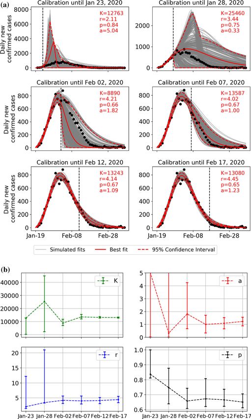
K. Wu et al.

responded efficiently and massively to this new           sensitive to the assumptions on the many often subtle
disease outbreak by implementing unprecedented            microscopic processes. Giving an illusion of preci-
containment measures to the whole country, includ-        sion, mechanistic models are sometimes quite fragile
ing lockdown of the whole province of Hubei and           and require an in-depth understanding of the domi-
putting most of other provinces in de facto quarantine    nating processes, which are likely to be missing in the
mode. Since March 2020, one and a half month after        confusion of an ongoing pandemics, with often
the national battle against the COVID-19 epidemic,        inconsistent and unreliable statistics and studies
China has managed to contain the virus transmission       performed under strong time pressure. There is thus
within the country, with new daily confirmed cases in     space for simpler and, we argue, more robust
mainland China excluding Hubei in the single digit        phenomenological models, which have low complex-
range, and with just double digit numbers in Hubei.       ity but enjoy robustness. This is the power of coarse-
In contrast, many other countries have had fast           graining, a well-known robust strategy to model
increasing numbers of confirmed cases since March         complex system [13–15].
2020, which leads to a resurgence in China due to the        Sophisticated statistical models including machine
imported cases from overseas. On March 11, the            learning techniques have also been utilized to study
World Health Organization (WHO) declared the              and predict the development of outbreaks in different
coronavirus outbreak as a global pandemic. As of          regions. For example, Gourieroux and Jasiak used
July 24, there are more than 15.5 million cases           time-varying Markov process to analyze the COVID-
confirmed in more than 210 countries and territories,     19 data [16]; Matthew Ekum and Adeyinka Ogun-
with 5.5 million active cases and approximately 640       sanya used hierarchical polynomial regression
thousand deaths.                                          models to predict transmission of COVID-19 at
    For an epidemic to develop, three key ingredients     global level [17]. These methods could potentially
are necessary: (1) source: pathogens and their reser-     provide good prediction results without detailed
voirs; (2) susceptible persons with a way for the virus   assumptions of underlying process; however, it is
to enter the body; (3) transmission: a path or            sometimes difficult to interpret the results and
mechanism by which viruses moved to other suscep-         understand the fundamental dynamics.
tible persons. Numerous mechanistic models based             In this paper, we focus on using phenomenological
on the classical SIR model and its extensions have        models without detailed microscopic foundations, but
been utilized to study the COVID-19 epidemic.             which have the advantage of allowing simple
Within such a multi-agent framework, one can detail       calibrations to the empirical reported data and
different attributes among countries, including the       providing transparent interpretations. Phenomenolog-
demographics, climate, population density, health-        ical approaches for modeling disease spread are
care systems, government interference, etc., which        particularly suitable when significant uncertainty
will affect the three key ingredients of the epidemic     clouds the epidemiology of an infectious disease,
mentioned above. There is a large amount of the           including the potential contribution of multiple
literature using this framework studying the past         transmission pathways [18]. In these situations,
major epidemics [1–6] as well as the current COVID-       phenomenological models provide a starting point
19 outbreak in different regions and countries [7–11].    for generating early estimates of the transmission
Notably, using such a framework, a report from Neil       potential and generating short-term forecasts of
Ferguson at Imperial College London [12] projected        epidemic trajectory and predictions of the final
future scenarios with different government strategies,    epidemic size [18].
which had a large impact on subsequent government            We employ the classical logistic growth model,
policies.                                                 the generalized logistic model (GLM), the general-
    The numerous underlying assumptions of this kind      ized Richards model (GRM) and the generalized
of models vary from one model to another, leading to      growth model (GGM), which have been successfully
a huge amount of publications presenting many types       applied to describe previous epidemics [18–22]. All
of results. These mechanistic models are useful in        these models have some limitations and are only
understanding the effect of different factors on the      applicable in some stages of the outbreak, or when
transmission process; however, they are highly            enough data points are available to allow for

123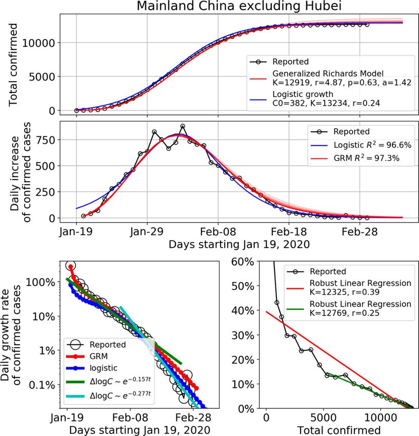
Generalized logistic growth modeling of the COVID-19 outbreak: comparing the dynamics

sufficiently stable calibration. For example, an epi-          issue of underreporting at the early stage and also
demic follows an exponential or quasi-exponential              data inconsistency during mid-February due to a
growth at an early stage (following the law of                 change of classification guidelines. For the provinces
proportional growth with multiplier equal to the basic         other than Hubei, the data are consistent except for
reproduction number R0), qualifying the generalized            one special event on February 20 concerning the data
growth model as more suitable in the initial regime.           coming from several prisons.
Then, the growth rate decays as fewer susceptible                 We do not include the Chinese domestic data after
people are available for infection and countermea-             March 10 because we conclude that the major
sures are introduced to hinder the transmission of the         outbreak between January and March was contained
virus, so the logistic type of models is better in this        and finished. Although there have been resurgences
later stage.                                                   of cases after mid-March due to imported cases from
    Our analysis dissects the development of the               overseas countries, it is another transmission dynam-
epidemics in China and the impact of the drastic               ics compared with the January–March major
control measures both at the aggregate level and               outbreak, and the risk of another round of epidemic
within each province. Borrowing from the experience            is low given the continuing containment measures
of China, we analyze the development of the outbreak           and massive testing programs [23].
in other countries. Our study employs simple models               For data in other countries, the source is the
to quantitatively document the effects of the Chinese          European Centre for Disease Prevention and Control
containment measures against the SARS-CoV-2                    (ECDC) [24], which is updated every day at 1 pm
virus, and provide informative implications for the            CET, reflecting data collected up to 6:00 and 10:00
current global pandemic. The quantitative analysis             CET. Note that the cases of the Diamond Princess
allows estimating the progress of the outbreak in              cruise are excluded from Japan, following the WHO
different countries, differentiating between those that        standard.
are at a quite advanced stage and close to the end of
the epidemics from those that are still in the middle of       2.2 Data adjustment
it. This is useful for scientific colleagues and decision
makers to understand the different dynamics and                On February 20, for the first time, infected cases in
status of countries and regions in a simple way.               the Chinese prison system were reported, including
    The paper is structured as follows: In Sect. 2 and 3,      271 cases from Hubei, 207 cases from Shandong, 34
we explain the data and the models in detail. In               cases from Zhejiang. These cases were concealed
Sect. 4 and 5, we calibrate different models to the            before this announcement because the prison system
reported number of infected cases in the COVID-19              was not within the coverage of each provincial health
epidemics from January 19 to March 10 for the whole            commission system. Given that the prison system is
of China and 29 provinces in mainland China. Then,             relatively independent and the cases are limited, we
in Sect. 6, we perform a similar modeling exercise on          remove these cases in our data for the modeling
other countries that have been or are undergoing               analysis to ensure consistency.
major outbreaks of this virus. We discuss several
limitations of our methods in Sect. 7 and then                 2.3 Migration data
conclude in Sect. 8.
                                                               The population travels from Hubei and Wuhan to
                                                               other provinces from January 1 to January 23 are
2 Data                                                         retrieved from the Baidu Migration Map (http://
                                                               qianxi.baidu.com).
2.1 Confirmed cases

We focus on the daily data of confirmed cases. For             3 Method
data from mainland China, the data source is national
and provincial heath commission. We exclude the                At an early stage of the outbreak, an exponential or
epicenter province, Hubei, which had a significant             generalized exponential model can be used to

                                                                                                           123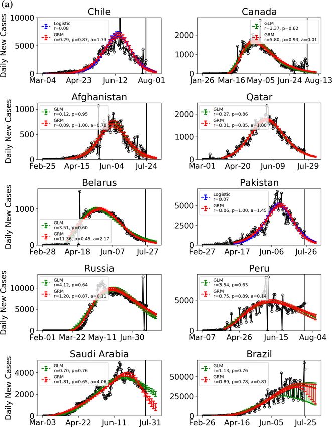
K. Wu et al.

describe the data, which is intuitive and easy to
                                                               dC ðtÞ     p        C ðt Þ
calibrate. This has been employed to describe the                     ¼ rC ðtÞ 1                                   ð3Þ
initial processes of the epidemic in many cases,                dt                  K
including influenza, Ebola, foot-and-mouth disease,            ●   Generalized Richards model (GRM):
HIV/AIDS, plague, measles, smallpox [20] and also
                                                               dC ðtÞ                       C ðt Þ a
COVID-19 [25]. The generalized growth model                           ¼ r ½ C ðt Þ p 1                            ð4Þ
(GGM) that we consider is defined as:                           dt                           K

dC ðtÞ
       ¼ rC p ðtÞ;                                      ð1Þ
 dt                                                               These three models all include two common
where CðtÞ represents the cumulative number of                 parameters: a generalized growth rate r setting the
confirmed cases at time t, p 2 ½0; 1 is an exponent           typical time scale of the epidemic growth process and
that allows the model to capture different growth              the final capacity K, which is the asymptotic total
profiles including the constant incidence (p ¼ 0), sub-        number of infections over the whole epidemics. In the
exponential growth (0\p\1) and exponential                     generalized logistic model, one additional parameter
growth (p ¼ 1). In the case of exponential growth,             p 2 ½0; 1 is introduced on top of the classical logistic
the solution is CðtÞ ¼ C0 ert , where r is the growth          model to capture different growth profiles, similar to
rate and C0 is the initial number of confirmed cases at        the generalized growth model (1). In the generalized
the time when the count starts. For                            Richards model, the exponent a is introduced to
                                            0\p\1,

                                                rt b
                                                         the
solution of Eq. (1)        is C ð t Þ ¼ C0  1 þ A    , where   measure the deviation from the symmetric S-shaped
                   C01p
b ¼ 1p1
          and A ¼ 1p    , so that r controls the charac-      dynamics of the simple logistic curve. The GRM
teristic time scale of the dynamics. Essentially, the          recovers the original Richards model [28] for p ¼ 1,
(quasi) exponential model provides an upper bound              and reduces to the classical logistic model (2) for
for future scenarios by assuming that the outbreak             a ¼ 1 and p ¼ 1. Therefore, the GRM is more
continues to grow following the same process as in             pertinent when calibrating data from a region that
the past.                                                      has entered the after-peak stage, to better describe the
   However, an outbreak will slow down and reach               after-peak trajectory that may have deviated from the
its limit with decaying transmission rate in the end,          classical logistic decay due, for instance, to various
resulting in the growth pattern departing from the             containment measures. However, this more flexible
(sub-)exponential path as the cumulative number of             model leads to more unstable calibrations if used on
cases approaches its inflection point and the daily            early stage data.
incidence curve approaches its maximum. Then, a                   For the calibrations performed here, we use the
logistic type model could have a better performance.           standard Levenberg–Marquardt algorithm to solve
In fact, the exponential model and the classical               the nonlinear least square optimization for the
logistic model are the first- and second-order approx-         incidence curve. This is achieved  by searching  for
imations to the growth phase of an epidemic curve                                            ^     ^  ^       ^
                                                               the set of parameters H ¼ h1 ; h2 ; . . .; hm that
produced by the standard Kermack–McKendrick SIR                minimizes        the    sum     of    squared      errors
                                                               PT                    2
model [26, 27]. To account for subtle differences in              t¼1 ðct  f ðt; HÞÞ , where f ðt; HÞ is the model
the dynamics of different stages of an epidemic, we            solution and ct is the observed data. For the fitting
use three types of logistic models to describe the             of the classical logistic growth function, we free the
outbreak beyond the early growth stage:                        initial point C0 and allow it to be one of the 3
                                                               parameters Hlog i ¼ ðC0 ; K; r Þ to be calibrated, as the
●   Classical Logistic growing model:
                                                               early stage growth does not follow a logistic growth.

dC ðtÞ               C ðt Þ                                    However, for the fitting of the remaining three
       ¼ rC ðtÞ 1                                      ð2Þ
 dt                   K                                        models, C0 is fixed at the empirical value. To
                                                               estimate the uncertainty of our model estimates, we
●   Generalized Logistic model (GLM):                          use a bootstrap approach with a negative binomial
                                                               error structure NBðlt ; r2t ), where lt and r2t are the
                                                               mean and variance of the distribution at time t,

123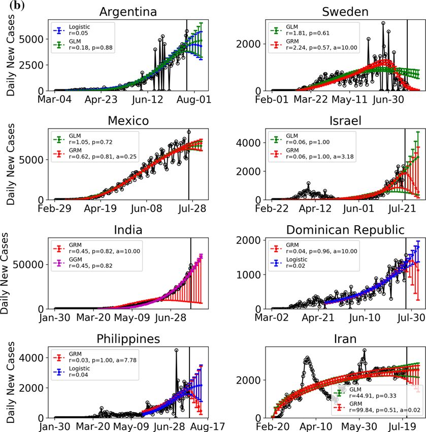
Generalized logistic growth modeling of the COVID-19 outbreak: comparing the dynamics

estimated from the empirical data. Concretely, we                      numbers and they both require more data to calibrate.
employ the following bootstrap step to simulate                        The performance of more flexible models increases as
S ¼ 500 time series:                                                   more data (especially data after the inflection point of
                                                                       the cumulative number) become available for cali-
  Step 1 Search for           the set of parameters
   ^ ¼ h^1 ; h^2 ; . . .; h^m that minimizes the sum of                bration. Given the above, we define three scenarios
  H
                      P                                                that can be described by these four models. The
  squared errors Tt¼1 ðct  f ðt; HÞÞ2 .                               positive scenario is defined by the model with the
  Step
          2        Each        simulated       time       series     second lowest predicted final total confirmed cases
  fi t; H^ ; i ¼ 1; 2; . . .; S is generated by assuming              K among the three Logistic models, and the medium
  a negative binomial error structure as NBðlt ; r2t ),                scenario is described by the model with the highest
                                                           f ðt;H
                                                                  ^Þ
  where            lt ¼ f t; H  ^           and       r2t ¼ T
                                                                       predicted final total deaths among the three Logistic
                                                                       models. It is important to note that both positive and
  PT ðcl f ðl;H^ ÞÞ2
      l¼1       ci      ; t ¼ 1; 2; . . .; T. Thus, the proba-         medium scenarios could underestimate largely the
  bility                          of                      success      final capacity, especially at the early stage of the
                                                    1               epidemics. The negative scenario is described by the
                                PT ðcl f ðl;H^ ÞÞ 2

  pt ¼ 1  rl2t ¼ 1  T             l¼1      ci            in a        generalized growth model, which should only
               t
                                                                       describe the early stage of the epidemic outbreak
  classical negative binomial distribution is the same
                                                                       and is therefore least reliable for countries in the
  across t.
                                                                       more mature stage as it does not include a finite
  Step 3 For each simulated time series, the param-
             ^ i ; i ¼ 1; 2; . . .; S is estimated as in Step 1.       population capacity.
  eter set H
  Thus, the empirical distribution, correlations and
  confidence intervals of the parameters and the
                                                         ^             4 Analysis at the global and provincial level
  model
          solution can be extracted from Hi and                        for China (excluding Hubei)
       ^ i , where i ¼ 1; 2; . . .; S.
  fi t; H
   In the next section, we apply the most flexible                     4.1 Analysis at the aggregate level of mainland
model, the generalized Richards model (GRM), to                            China (excluding Hubei)
study the 29 provinces in China where the outbreak is
at the end. The GRM has four free parameters                           As of March 10, 2020, there were in total 13,172
(HGRM ¼ ðK; r; p; a)) and is able to characterize the                  infected cases reported in the 30 provinces in
different epidemic patterns developed in the 29                        mainland China outside Hubei. The initially impres-
provinces. We also fit the classical logistic model to                 sive rising statistics have given place to a tapering
the daily incidence data as a comparison with the                      associated with the limited capacity for transmission,
GRM, and a simple exponential decay model to the                       exogenous control measure, and so on. In Fig. 1, the
growth rate of cumulative confirmed cases to provide                   trajectory of the total confirmed cases, the daily
another perspective.                                                   increase of confirmed cases and the daily growth rate
   In Sect. 6, we apply the four models (Eqs. 1–4) to                  of confirmed cases in whole China excluding Hubei
various countries and regions to identify their                        province are presented. The fits with the generalized
epidemic progress and potential future scenarios.                      Richards model and with the classical logistic growth
Logistic type models tend to underestimate the final                   model are shown in red and blue lines, respectively,
capacity K and thus could serve as lower bounds of                     in the upper, middle and lower left panel, with the
the future scenarios [29, 30]. The classical logistic                  data up to March 1, 2020. In the lower left panel of
model is the least flexible one among the three and                    Fig. 1, the daily empirical growth rate
usually provides the lowest estimate of the final                      r ðtÞ ¼ log CCðt1
                                                                                       ðt Þ
                                                                                            Þ of the confirmed cases is plotted in
capacity, because it fails to account for (1) the sup-                 log scale against time. We can observe two expo-
exponential growth which could be captured by the                      nential decay regimes of the growth rate with two
GLM; (2) the potential slow abating of the epidemic                    different decay parameters before and after February
which could be captured by the GRM. Both factors                       14, 2020. The green line is the fitted linear regression
will increase the estimated final total confirmed                      line (of the logarithm of the growth rate as a function

                                                                                                                       123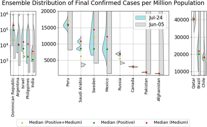
K. Wu et al.

Fig. 1 Time dependence of the total number of confirmed          robustness of the fits. The lower left panel shows the daily
cases (upper panel), the daily number of new confirmed cases     growth rate of the confirmed cases in log scale against time.
(middle panel), and the daily growth rate of confirmed cases     The green and cyan straight lines show the linear regression of
(lower panel) in the mainland China excluding Hubei province     the logarithm of the growth rate as a function of time for the
until March 1, 2020. The empirical data are marked by the        period of January 25 to February 14, and the period of February
empty circles. The blue and red lines in the upper, middle and   15 to March 1, respectively. The lower right panel is the daily
lower left panels show the fits with the logistic growth model   growth rate of the confirmed cases in linear scale against the
and generalized Richards model (GRM) respectively. For the       cumulative number of confirmed cases. The red and green lines
GRM, we also show the fits using data ending 20, 15, 10,         are the linear fits for the period of January 19 to February 1,
5 days earlier than March 1, 2020, as lighter red lines in the   and the period of February 2 to March 1, respectively
upper and middle panel. This demonstrates the consistency and

of time) for the data from January 25 to February 14,            February 15, 3 weeks after a series of extreme
2020, yielding an exponential decay parameter equal              controlling measures, the growth rate is found to
to −0.157 per day (95% CI: (−0.164, −0.150)). This               decay with a faster rate with a decay parameter equal
indicates that after the lockdown of Wuhan city on               to −0.277 per day (95% CI: (−0.313, −0.241)).
January 23 and the top-level health emergency                       This second regime is plotted as the cyan line in
activated in most provinces on January 25, the                   the lower left panel of Fig. 1. The green and cyan
transmission in provinces outside Hubei has been                 straight lines show the linear regression of the
contained with a relatively fast exponential decay of            logarithm of the growth rate as a function of time
the growth rate from a value starting at more than               for the period of January 25 to February 14, and the
100% to around 2% on February 14. Then, starting                 period of February 15 to March 1, respectively. The

123
Generalized logistic growth modeling of the COVID-19 outbreak: comparing the dynamics
asymptotic exponential decay of the growth rate can bootstrap with a negative binomial error structure, as
be justified theoretically from the generalized in prior studies [20]. Each of these 500 simulations
Richards model (4) by expanding it in the neighbor- constitutes a plausible scenario for the daily number
hood where C converges to K. Introducing the change of new confirmed cases, which is compatible with the
of variable CðtÞ ¼ K ð1 eðtÞÞ, and keeping all terms data and GRM. The dispersion among these 500
up to first order in eðtÞ, Eq. (4) yields scenarios provides a measure of stability of the fits,
and their range of values gives an estimation of the
dðtÞ
¼ ceðtÞ with c ¼ raK p1 : ð5Þ confidence intervals. The first conclusion is the non-
dt
surprising large range of scenarios obtained when
This gives using data before the inflection point, which, how-
1 dC ðtÞ 0 cect ever, encompass the realized data. We observe a
¼ ct
¼ c 0 ect þ ½0 ect 2 þ ½0 ect 3 þ ; tendency for early scenarios to predict a much faster
C dt 1 0 e
ð6Þ and larger number of new cases than observed, which
could be expected in the absence of strong contain-
where e0 is a constant of integration determined from ment control. With more data, the scenarios become
matching this asymptotic solution with the non- more accurate, especially when using realized data
asymptotic dynamics far from the asymptote. Thus, after the peak, and probably account well for the
the leading behavior of the growth rate at long times impact of the containment measures that modified the
is C1 dCdðt tÞ =c0 ect , which is exponential decaying as dynamics of the epidemic spreading. This is con-
shown in the lower left panel of Fig. 1. Using firmed again in Fig. 2b, which presents the
expression (5) for c as a function of the 4 parameters convergences of the four parameters of the GRM.
r; a; K and p given in the inset of the top panel of The confidence intervals decrease significantly once
Fig. 1, we get c ¼ 0:21 for mainland China excluding the data are available after the inflection point.
Hubei, which is bracketed by the two fitted values
0.17 and 0.28 of the exponential decay given in the 4.2 Analysis at the provincial level (29
inset of the lower left panel of Fig. 1. provinces) of mainland China (excluding
In the lower right panel of Fig. 1, the empirical Hubei)
growth rate r ðtÞ is plotted in linear scale against the
cumulative number of confirmed cases. The red and As of March 1, 2020, the daily increase of the number
green lines are the linear regressed lines for the full of confirmed cases in China excluding Hubei
period and for the period after February 1, 2020, province has decreased to less than 10 cases per
respectively. We can see that the standard logistic day. The preceding one-month extreme quarantine
growth cannot capture the full trajectory until Febru- measures thus seem to have been very effective from
ary 1. After February 1, the linear fit is good, an aggregate perspective, although there is a resur-
qualifying the simple logistic equation (p=1 and α= gence of cases since mid-March due to imported
1), with growth rate r estimated as 0.25 for the slope, cases from overseas countries. At this time, it is
which is compatible with the value determined from worthwhile to take a closer look at the provincial
the calibration over the full data set shown in the top level to study the effectiveness of measures in each
two panels of Fig. 1. province. The supplementary material presents fig-
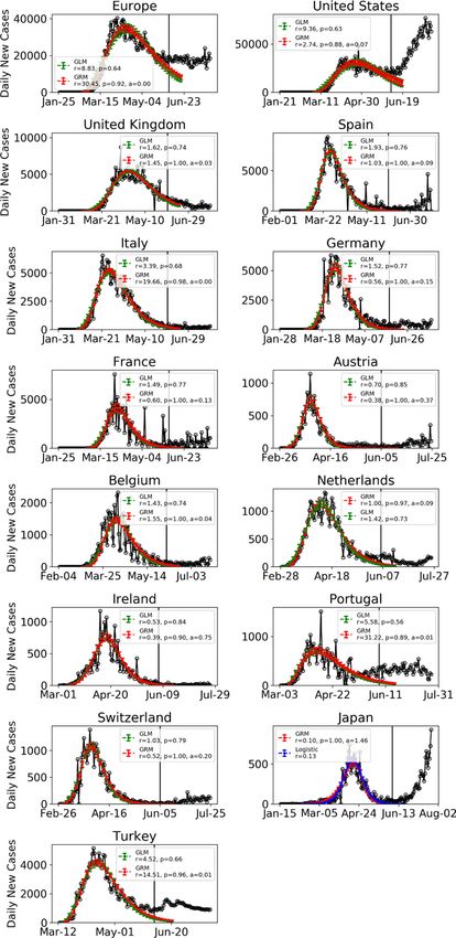
Figure 2a demonstrates the sensitivity of the ures similar to Fig. 1 for each of the 29 provinces in
calibration of the GRM to the end date of the data mainland China, and a table presenting some useful
by presenting six sets of results for six end dates. statistics for each province and the values of the fitted
Specifically, the data on the daily number of new parameters of the generalized Richards model, logis-
confirmed case are assumed to be available until 23 tic growth model and the exponential decay exponent
January, 28 January, 2 February, 7 February, 12 of the growth rate. Tibet is excluded as it only has 1
February, 17 February, i.e., 30, 25, 20, 15, 10 and confirmed case as of March 10. This analysis at the
5 days before February 22 were presented. For each 29 provinces allows us to identify four phases in the
of the six data sets, we generated 500 simulations of development of the epidemic outbreak in mainland
dCðtÞ based on the best fit parameters using parametric
dt China.
123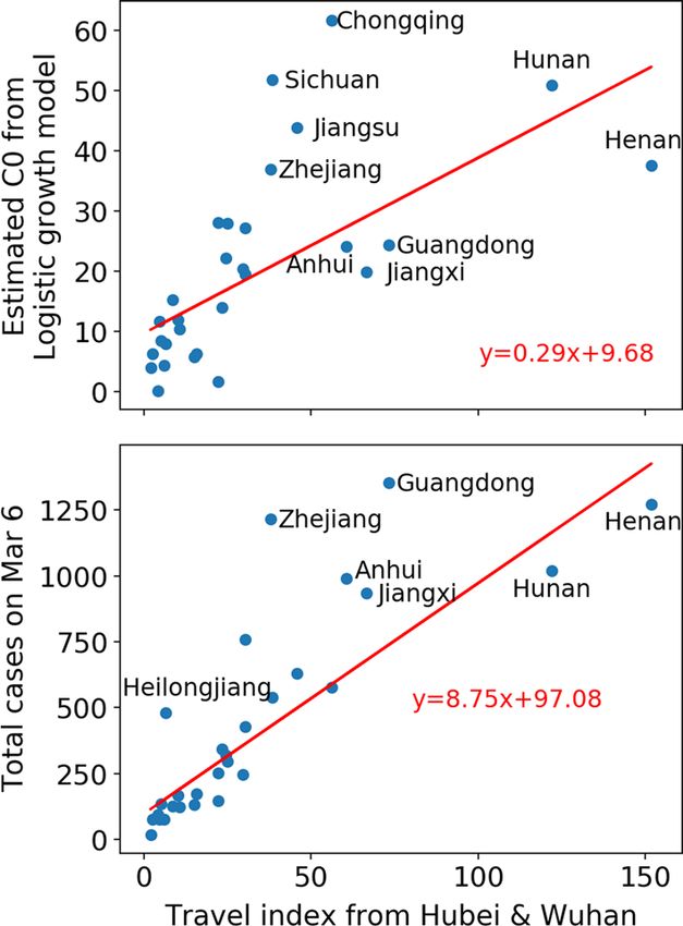
K. Wu et al.

Fig. 2 a Daily number of
new observed confirmed
cases for mainland China
excluding Hubei (black
circles) compared with 500
scenarios built by
parametric bootstrap with a
negative binomial error
structure on the GRM
model with best fit
parameters determined on
the data up to the time
indicated by the vertical
dashed line. The last time
used in the calibration is,
respectively, 5, 10, 15, 20,
25, 30 days before February
22, 2020 from bottom to
top. The red continuous line
is the best fitted line, and
the two dashed red curves
delineate the 95%
confidence interval
extracted from the 500
scenarios. The six panels
correspond each to a
different end date, shown as
the sub-title of each panel,
at which the data have been
calibrated with the GRM
model. b Convergence of
the four parameters from
the GRM simulations
shown in a. The error bars
indicate the 80% prediction
intervals. (Color
figure online)

123
Generalized logistic growth modeling of the COVID-19 outbreak: comparing the dynamics
● Phase I (January 19–January 24, 6 days): early implement their strict measures, striving to bring
stage outbreak The data mainly reflect the the epidemics to an end. The growth rate of the
situation before January 20, when no measures number of confirmed cases declined exponen-
were implemented, or they were of limited scope. tially with similar rates as in Phase II, pushing
On January 19, Guangdong became the first down the growth rate from 10 to 1%. In phase III,
province to declare a confirmed case outside all provinces have passed the peak of the
Hubei in mainland China [22]. On January 20, incidence curve, which allows us to obtain precise
with the speech of President Xi, all provinces scenarios for the dynamics of the end of the
started to react. As of January 24, 28 provinces outbreak from the model fits (Fig. 2). As of
reported confirmed cases with daily growth rates February 14, 23 out of 30 provinces have less
of confirmed cases ranging from 50% to more than 10 new cases per day.
than 100%. ● Phase IV (February 15–8 March) the end of the
● Phase II (January 25–February 1, 8 days) fast outbreak Starting February 15, the exponential
growth phase approaching the peak of the decay of the growth rate at the aggregate level has
incidence curve (inflection point of the cumulative switched to an even faster decay with parameter
number) The data start to reflect the measures of 0.277 (Fig. 1). As of February 17, 1 week after
implemented in the later days of Phase I and in normal work being allowed to resume in most
Phase II. In this phase, the government measures provinces, 22 provinces have a growth rate
against the outbreak have been escalated, marked smaller than 1%. As of February 21, 28 provinces
by the lockdown of Wuhan on January 23, the have achieved 5-day average growth rates smaller
top-level public health emergency state declared than 1%.
by 20+provinces by January 25, and the standing
committee meeting on January 25, the first day of
the Chinese New Year, organized by President
Xi, to deploy the forces for the battle against the 5 Analysis of the development of the epidemic
virus outbreak. In this phase, the growth rate of and heterogeneous Chinese provincial responses
the number of confirmed cases in all provinces
declined from 50 to 10%+, with an exponentially 5.1 Quantification of the initial reactions
decay rate of 0.157 for the aggregated data. At the and ramping up of control measures
provincial level, some provinces failed to see a
continuous decrease in the growth rate and On January 19, Guangdong was the first province to
witnessed the incidence grow at a constant rate report a confirmed infected patient outside Hubei. On
for a few days, implying exponential growth of January 20, 14 provinces reported their own first case.
the confirmed cases. These provinces include During January 21–23, another 14 provinces reported
Jiangxi (~40% until January 30), Heilongjiang (~ their first cases. If we determine the peak of the
25% until February 5), Beijing (~15% until outbreak from the 5 days moving average of the
February 3), Shanghai (~20% until January 30), incidence curve, then there are 15 provinces taking 7–
Yunnan (~75% until January 27), Hainan (~10% 11 days from their first case to their peak, 9 provinces
until February 5), Guizhou (~25% until February taking 12–15 days and 6 provinces taking more than
1), Jilin (~30% until February 3). Some other 15 days. If we define the end of the outbreak as the
provinces managed to decrease the growth rate day when the 5 days moving average of the growth
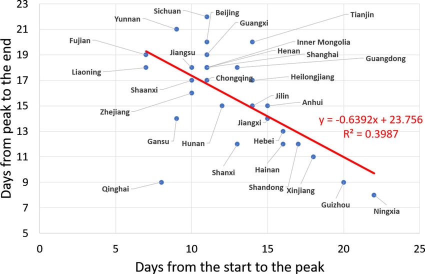
exponentially during this period. As of February rate becomes smaller than 1%, then 7 provinces spent
1, 15 provinces had reached the peak of the 8–12 days from the peak to the end, 7 provinces spent
incidence curve, indicating the effectiveness of 13–16 days, 13 provinces spent 17–20 days and 2
the extreme measures, and most provinces started provinces spent 21–22 days. For the six provinces
to be in control of the epidemics. that have the longest duration from the start of their
● Phase III (February 2–February 14, 13 days) slow outbreak to the peak (more than 15 days), it took 8–
growth phase approaching the end of the outbreak 13 days for them to see the end of the outbreak
In this period, all provinces continued to (Fig. 3). This means that these 6 provinces were able
123K. Wu et al.
Fig. 3 Inverse relationship
found across the 29 Chinese
provinces between the
number of days from peak
to the end and the duration
from start to the peak of the
epidemics. Here, the end of
the outbreak is defined
operationally as the day
when the 5 days moving
average of the growth rate
becomes smaller than 1%
to control the local transmissions of the imported 5.3 Zhejiang and Henan exemplary developments
cases quite well, so that the secondary transmissions
were limited. In contrast, 20 provinces took 28– Zhejiang and Henan are the second and third most
31 days from the start to the end of the outbreak. infected provinces but have the fastest decaying
Thus, those provinces that seem to have responded speed of the incidence growth rate (exponential decay
sluggishly during the early phase of the epidemics exponent for Zhejiang: 0.223, Hunan: 0.186) among
seem to have ramped up aggressively their counter- the most infected provinces. This is consistent with
measures to achieve good results. the fast and strong control measures enforced by both
provincial governments, which have been praised a
5.2 Diagnostic of the efficiency of control lot on Chinese social network [31, 32]. As one of the
measures from the exponential decay most active economies in China and one of the top
of the growth rate of infected cases provinces receiving travelers from Wuhan around the
Lunar New Year [33], Zhejiang was the first province
The 10 most infected provinces (Guangdong, Henan, launching the top-level public health emergency on
Zhejiang, Hunan, Anhui, Jiangxi, Shandong, Jiangsu, January 23, and implemented strong immediate
Chongqing, Sichuan) have done quite well in con- measures, such as closing off all villages in some
trolling the transmission, as indicated by the fact that cities. The fitted curves from the GRM and logistic
their daily growth rates follow well-defined expo- growth models indicate a peak of the incidence curve
nential decays, with all of their R2 larger than 90%. on January 31, which is the earliest time among top
This exponential decay continued for all ten pro- infected provinces. Similarly, Henan Province, as the
vinces until the situation was completely under neighbor province of Hubei and one of the most
control during February 15–18, when the daily populated provinces in China, announced the sus-
incidence was at near zero or a single-digit number. pension of passenger bus to and from Wuhan at the
Eight out of these ten provinces have an exponential end of December 2019. In early January 2020, Henan
decay exponent of the growth rate ranging from 0.142 implemented a series of actions including suspending
to 0.173, similar to what is observed at the national poultry trading, setting up return spots at the village
average level (0.157). Note that this exponential entrances for people from Hubei, listing designated
decay can be inferred from the generalized Richards hospitals for COVID-19 starting as early as January
model, as we noted in Eqs. (5) and (6) in Sect. 4.1. 17, and so on [32]. These actions were the first to be
implemented among all provinces.
123Generalized logistic growth modeling of the COVID-19 outbreak: comparing the dynamics
5.4 Heterogeneity of the development
of the epidemic and responses across various
provinces
Less infected provinces exhibit a larger variance in
the decaying process of the growth rate. However, we
also see good examples like Shanghai, Fujian and
Shanxi, which were able to reduce the growth rate
consistently with a low variance. These provinces
benefited from experience obtained in the fight
against the 2003 SARS outbreak or enjoy richer
local medical resources [34]. This enabled the
government to identify as many infected/suspected
cases as possible in order to contain continuously the
local transmissions. Bad examples include Hei-
longjiang, Jilin, Tianjin, Gansu, which is consistent
with the analysis of [34].
Most provinces have a small parameter of p in the
GRM [see Eq. (4)] and an exponent α large than 1,
indicating that China was successful in containing the
Fig. 4 Upper panel: estimated C0 for the logistic growth
outbreak as sub-exponential growing process (p\1), model versus travel index from Hubei and Wuhan. Lower
with a faster than logistic decay (α[1) in most panel: total confirmed cases versus travel index from Hubei
provinces, except Guangdong, Zhejiang, Jiangxi, and Wuhan. The Pearson correlation between C0 and the
migration index is 0.65 (p\103 ), and the correlation between
Sichuan, Heilongjiang, Fujian, Yunnan and Gansu.
the cumulative number of confirmed cases and the migration
However, these exceptional provinces are due to various index is 0.82 (p\104 )
reasons, which may not necessarily be the ineffective
measures. The large p and small α in Guangdong and level of early contamination from Hubei province as the
Zhejiang are likely due to their high population densities epicenter of the outbreak. To support this proposition, the
and highly mobile populations in mega-cities, which are upper panel of Fig. 4 plots the estimated C0 as a function
factors known to largely contribute to the fast transmis- of the migration index from Hubei and Wuhan to each
sion of viruses. Jiangxi, Sichuan, Fujian, Yunnan and province. The migration index is calculated as equal to
Gansu all had a fast growth phase before February 1, but 25% of the population migrating from Hubei (excluding
were successful in controlling the subsequent develop- Wuhan) plus 75% of the population migrating from
ment of the epidemics. The fast growth phase in Wuhan, given that Wuhan was the epicenter and the risks
Heilongjiang lasted a bit longer than the above- from the Hubei region excluding Wuhan are lower. One
mentioned provinces, due to the occurrence of numerous can observe a clear positive correlation between the
local transmissions. Heilongjiang is the northernmost estimated C0 and the migration index. The lower panel of
province in China, so it is far from Hubei and does not Fig. 4 shows an even stronger correlation between the
have a large number of migrating people from Hubei. total number of cases recorded on March 6 and the travel
However, compared with other provinces, it has a high index, expressing that a strong start of the epidemics
statistic of both the confirmed cases and the case fatality predicts a larger number of cases, which is augmented by
rate (2.7% as of March 10), which has been criticized a infections resulting from migrations out of the epidemic
lot by the Chinese social network. epicenter.
5.5 Initial and total confirmed numbers
of infected cases correlated with travel index 6 Analysis of the epidemic in various countries
The initial value C0 of the logistic equation could be used Based on the phenomenological models presented
as an indicator of the early number of cases, reflecting the above, we have been publishing daily forecasts for
123K. Wu et al.
the number of COVID-19 confirmed cases in various the after-peak trajectory in an epidemic, it cannot
countries/regions in the world since March 23. Four characterize the second wave dynamics by construc-
months after our first daily report, the outbreaks in tion. Therefore, we use June 5 as the cutoff date for
most European countries have come to an end and the the data used in the exercise of model fitting to
epicenter has shifted to the USA, South Hemisphere Europe as a whole and to 14 countries that have
countries and other developing countries. In this ended their first waves. These countries are the USA,
section, with the four models (Eqs. 1–4) and the 11 west European countries (the UK, Spain, Italy,
resulting three scenarios we specified in Sect. 3, we Germany, France, Austria, Belgium, Netherlands,
first present the model outputs for countries with an Ireland, Portugal and Switzerland) and two Asian
ended first outbreak wave. We report that they have countries (Japan and Turkey). Among these 14
significantly different parameters compared to China. countries, a second wave of outbreak has started in
Then, we present the latest status of the countries in the USA and Japan. Resurgences of cases are
the middle of their outbreak and discuss the perfor- identified in several countries including Spain, Ger-
mance of our models. many, France, Austria, Portugal, Switzerland and
Turkey.
6.1 Countries with a matured outbreak Figure 5 presents the daily confirmed cases of
Europe and of 14 countries fitted with the best two
As of July 24, Europe (including Russia) has models among the four models. In contrast to the
cumulatively 3.06 million confirmed cases with a results from most provinces in China in the after-peak
growth rate of 0.5–1% per day, gradually decreased stage, all West European countries have a small
from more than 5% 2 months ago. The outbreak in estimated parameter α in the generalized Richards
Europe started in February from Italy, France and model, indicating a slow decay of the after-peak
Spain and then spread to the whole Europe. The first trajectory. This is possibly because the full lockdown
wave of outbreaks has ended in most West European in most West European countries was implemented
countries, which started to ease their lockdowns in when the virus transmissions have already started
late April. However, the rising numbers of cases in among local communities. The heterogeneous stage
the East European countries (especially Russia) and of the outbreaks and the resurgences of cases in some
the resurgences of cases in the West European countries (e.g., Spain, German, France, Austria,
countries since June have kept the daily number of Portugal, Switzerland) also contribute to a slow
confirmed cases in Europe approximately flat after decay of Europe as a whole, which is in an
May. approximate plateau over the past month. In contrast,
As of July 24, the USA has cumulatively 4.03 the extreme lockdown and containment measures in
million confirmed cases with a daily growth rate of China were implemented at the beginning of the
around 2%, increased from 1% a month ago. The first outbreak and were maintained strictly through the
wave of outbreaks in the USA was concentrating in whole period of the outbreak with centralized man-
New York with a national lockdown from March to agement, contributing to the fast decay of the
late April. However, with the pressure from people in outbreak in the after-peak stage.
several states and from President Trump, the USA The resurgences of cases and a second wave
reopened since May. The ease of lockdowns and the happening in the USA and various countries show
street demonstrations associated with the BLM (“black that the risk of new outbreaks is not negligible. The
lives matter”) movement where large numbers of antibody tests performed in various countries and
people gather have contributed to a second wave of regions [35] also show that the herd immunity level
outbreaks across the whole country, with the daily new in the crowd is not yet sufficient to prevent another
cases of the USA keeping breaking records. The outbreak.
epicenter of this second wave of the outbreak has
shifted from New York to several states such as 6.2 Countries in the middle of their outbreaks
Alabama, Arkansas, Arizona, California and Florida.
Although the flexible four-parameter generalized In Table 1, we report the latest confirmed cases per
Richards model (GRM) can capture the slow decay of million population and the estimated outbreak
123Generalized logistic growth modeling of the COVID-19 outbreak: comparing the dynamics
Fig. 5 Daily confirmed
cases of Europe and of 14
countries with the best two
models among the four
models (1)–(4). The
empirical data are indicated
by empty circles. The blue,
red and green lines with the
error bars show the fits with
the logistic growth model,
generalized Richards model
(GRM), and generalized
logistic model (GLM),
respectively. The error bars
indicate 80% prediction
intervals. Data are plotted
every 3 days. The vertical
line indicates the date (June
5) up to when the data are
fed to the model. (Color
figure online)
123K. Wu et al.
Table 1 Current confirmed cases per million population and estimated outbreak progress in positive and medium scenarios (July 24
confirmed cases divided by the estimated total final confirmed cases in positive and medium scenario)
Confirmed per million Outbreak progress Outbreak progress
population (July 24) in positive scenario in medium scenario
Chile 18,087 99.4% 98.3%
(60.2%, 100.0%) (53.1%, 100.0%)
Canada 3040 98.9% 97.2%
(95.2%, 100.0%) (93.9%, 100.0%)
Afghanistan 967 96.9% 96.4%
(91.5%, 100.0%) (90.4%, 100.0%)
Qatar 38,913 96.5% 95.6%
(94.4%, 98.4%) (93.3%, 97.8%)
Belarus 7031 94.0% 91.6%
(92.0%, 96.3%) (89.5%, 93.8%)
Pakistan 1274 95.8% 88.2%
(92.6%, 98.8%) (85.2%, 91.2%)
Russia 5503 80.4% 77.1%
(75.9%, 84.7%) (73.6%, 80.9%)
Peru 11,601 73.8% 72.5%
(68.5%, 79.1%) (65.7%, 79.6%)
Saudi Arabia 7727 89.9% 71.4%
(85.4%, 93.7%) (67.3%, 75.4%)
Sweden 7735 90.5% 53.7%
(82.5%, 99.8%) (38.7%, 65.5%)
Brazil 10,920 54.2% 49.6%
(36.8%, 79.6%) (38.6%, 97.2%)
Argentina 3189 30.0% 26.9%
(8.5%, 47.7%) (8.4%, 77.4%)
Mexico 2938 35.1% 23.9%
(27.6%, 42.3%) (14.0%, 45.7%)
Israel 6527 100.0% Not reliable
(23.1%, 100.0%)
India 952 78.0% 23.0%
(17.7%, 100.0%) (14.3%, 31.7%)
Dominican Republic 5421 Not reliable Not reliable
Philippines 698 Not reliable Not reliable
Iran 3472 Not reliable Not reliable
The ranking is in terms of outbreak progress in medium scenario (fourth column from left). Numbers in brackets are 80% confidence
intervals. As positive scenarios predict a smaller final number of total infected cases, the outbreak progress is thus larger in the
positive scenario
progress in the positive and medium scenarios for cases divided by the estimated final total confirmed
various countries including Chile, Canada, Afghani- case, either in the positive or the medium scenario. In
stan, Qatar, Belarus, Pakistan, Russia, Peru, Saudi Fig. 6, the daily confirmed cases of these 18 countries
Arabia, Brazil, Argentina, Sweden, Mexico, Israel, are shown together with the best two models among
India, Dominican Republic, Philippines and Iran. The the four models (1)–(4). Figure 7 presents the
outbreak progress is defined as the latest confirmed ensemble distribution of the estimated final total
123Generalized logistic growth modeling of the COVID-19 outbreak: comparing the dynamics
Fig. 6 a Daily confirmed
cases of 10 countries with
the best two models among
the four models (1)–(4). The
empirical data are indicated
by empty circles. The blue,
red and green lines with the
error bars show the fits with
the logistic growth model,
generalized Richards model
(GRM) and generalized
logistic model (GLM),
respectively. The error bars
indicate 80% prediction
intervals. Data are plotted
every 3 days. The vertical
line indicates the date (July
24) up to when the data are
fed to the model. b Daily
confirmed cases of 8
countries with the best two
models among the four
models (1)–(4). The
empirical data are indicated
by empty circles. The blue,
red and green lines with the
error bars show the fits with
the logistic growth model,
generalized Richards model
(GRM) and generalized
logistic model (GLM),
respectively. The error bars
indicate 80% prediction
intervals. Data are plotted
every 3 days. The vertical
line indicates the date (July
24) up to when the data are
fed to the model. (Color
figure online)
confirmed cases per million population obtained by and Saudi Arabia, which are less matured with
aggregating the positive and medium scenarios. The outbreak progress in the range 60–90% in the
distributions obtained on June 6, 2020, are plotted on medium scenario. They have developed signs of
the right side of each violin plot in gray, while the passing their inflection points, but may reverse to
distributions obtained on July 24 are plotted on the their previous exponential growth if there is a second
left side in cyan. wave of outbreak. All these countries have their
Among them, the most matured group of countries distributions of final confirmed cases converged,
includes Chile, Canada, Afghanistan, Qatar and indicating the reliability of the future projected
Belarus, which have strong signs that their inflection scenarios.
points have been passed with an outbreak progress The least mature group of countries are Sweden,
larger than 90% in the medium scenario. The next Brazil, Argentina, Mexico, Israel, India, Dominican
group of countries includes Pakistan, Russia, Peru Republic, Philippines and Iran. Sweden, Israel,
123K. Wu et al. Fig. 6 continued Philippines and Iran are experiencing a second estimated outbreak progress serves both as a lower outbreak, while Brazil, Argentina, Mexico, India bound for future developments and as an indication of and Dominican Republic are still in the exponential what to expect of the evolution dynamics of the growth stage, indicating highly uncertain future epidemics. To have a view of the performance of projections. As shown in Fig. 7, their ensemble short-term predictions, we present the latest 7-day distributions of final confirmed cases are non-con- prediction errors for the total number of confirmed verged or highly dispersed. cases in Fig. 8, based on positive and medium As discussed before, our models are unable to scenarios. One can see that our 7-day predictions characterize the second wave dynamics by construc- based on the data up to July 17 are correct with narrow tion. Thus, the results concerning the predictions for prediction intervals in all matured countries. Our 7-day countries experiencing a second wave are not reliable. predictions, however, underestimate the realized val- Note that the logistic type models are usually useful in ues in immature countries including India, Argentina understanding the short-term dynamics over a horizon and Israel. Until May 24, 2020, we have uploaded a of a few days, while may tend to underestimate long- daily update of our projections and an analysis of term results due to the change of the fundamental forecasting errors online [36]. Thereafter, we shifted to dynamics resulting from government interventions, a a weekly update until July 3, we have now discontin- second wave of outbreaks or other factors. This is ued it as the epidemics have entered second waves and shown by large shifts between the obtained distribu- other regimes highly dependent on country specific tions between June 5 and July 24 in Fig. 7. Thus, the characteristics. 123
Generalized logistic growth modeling of the COVID-19 outbreak: comparing the dynamics

Fig. 7 Violin plot of the distributions of the final total number   negative scenario does not incorporate a maximum saturation
of confirmed cases per million derived by combining the             number and thus cannot be used. The yellow dots indicate the
distributions of the positive and medium scenarios. The left        median prediction for the combined distribution, while the
side of each violin in cyan shows distributions obtained on July    green and red dots indicate the median of the positive and of
24, while the right side of each violin in gray shows               the medium scenarios, respectively. (Color figure online)
distributions obtained on June 5. The model setup in the

Fig. 8 7-day prediction
error of the forecast
performed on July 17 for
the total number of deaths
for various countries/
regions. The horizontal line
corresponds to the empirical
data on July 24. The error
bars are 80% prediction
intervals, and the middle
dots are the median
predictions based on the
predictions from the
positive and medium
scenarios. A negative value
corresponds to a prediction
that underestimated the true
realized value

7 Discussion on the limitation of the method                        statistic to estimate the true situation of the outbreak
                                                                    in a country, and we lay out four major variables
In this paper, we only apply the models to the number               here:
of confirmed cases, which is largely subject to a
                                                                    ●   Case definition Different countries employ differ-
number of extraneous variations among countries
                                                                        ent definitions of a confirmed COVID-19 case,
such as case definition, testing capacity, testing
                                                                        and the definition also changes over the time. For
protocol and reporting system. It is important to note
                                                                        example, China’s national health commission
that there is a significant limitation in using this

                                                                                                                     123
K. Wu et al.
issued seven versions of a case definition for Moreover, factors like heterogeneous demograph-
COVID-19 between 15 January and 3 March, and ics, government response, people’s fundamental
a recent study found each of the first four changes health situations in different countries could lead to
increased the proportion of cases detected and significantly different susceptibility to SARS-CoV-2.
counted by factors between 2.8 and 7.1 [37]. Numerous evidences are showing that the main
● Testing capacity The number of confirmed cases vulnerable group in this COVID-19 pandemic is the
is usually determined by testing, which is biased older population or people with preexisting chronic
toward severe cases in some countries like diseases, such as cardiovascular disease, hyperten-
France. In contrast, the testing is aimed at a sion, diabetes and with obesity [42–45]. The
larger group in some other countries implement- discipline and distanciation culture in some Asian
ing massive testing programs, such as South countries may also have contributed to the low
Korea and Iceland. Based on antibody tests number of confirmed cases there. All these factors
performed on the general population, several affect the susceptibility of individuals and the trans-
reports show that the actual number of infected mission networks, which are not easy to handle in a
people is much larger than the reported value microscopic model.
[38, 39]. Therefore our top-down approach could be useful
● Testing protocol The testing protocols and accu- in quantifying and understanding the current status of
racy may also have a large impact on the results. the outbreak progress and making short-term predic-
Depending on the testing protocols used, in some tions, while they tend to underestimate the final
instances, false positive results have been confirmed numbers in the long term, which has a
obtained. In other words, someone without the higher uncertainty. Thus, the three Logistic type
disease tested positive, probably because they models could only provide a lower bound for the
were infected with some other coronavirus. There future scenarios. As more data become available, we
have been several reports raising this issue [40]. anticipate a more accurate picture of the final
On the other hand, false negative results may also numbers, as showed, for instance, by the converged
exist and seem to be more prevalent than false ensemble distributions in Austria and Switzerland
positives. with small variance. As a last remark, even if the true
● Reporting system and time Data also rely on the number of cases is a multiple of the reported number
efficiency of the reporting system. Tests are of confirmed cases, as long as the multiple does not
conducted sequentially over time, and the vary too much for a given country, our analysis
reported data may be adjusted afterward. They remains pertinent to ascertain the outbreak progress
do not represent a snapshot of a day in time. For and nature of the epidemic dynamics.
instance, the Netherlands National Institute for
Public Health and the Environment clearly states
that some of the positive results are only reported 8 Conclusion
one or a few days later and there might be
corrections for the past data, so the numbers from In this paper, we calibrated the logistic growth model,
a few days ago are sometimes adjusted [41]. the generalized logistic growth model, the general-
ized growth model and the generalized Richards
Therefore, the real number of cases in the popu-
model to the reported number of confirmed cases in
lation is likely to be many multiples higher than those
the Covid-19 epidemics from January 19 to March 10
computed from confirmed tests, and the number of
for the whole of China and for the 29 provinces in
confirmed cases can only reflect the real situation of
China. This has allowed us to draw some lessons
the outbreak to some degree. This may also partly
useful to interpret the results of a similar modeling
explain that the Logistic model fails to capture the
exercise performed on other countries, which are at
growth dynamics at the early stage in most provinces
less advanced stages of their outbreaks. Our analysis
in China, as shown in Sect. 5, likely due to the
dissects the development of the epidemics in China
potential underreporting at the beginning.
and the impact of the drastic control measures both at
the aggregate level and within each province. We
123You can also read