Global Syntactic Variation in Seven Languages: Towards a Computational Dialectology
←
→
Page content transcription
If your browser does not render page correctly, please read the page content below
Global Syntactic Variation in Seven
                                        Languages: Towards a Computational
                                        Dialectology
                                        Jonathan Dunn 1,∗
                                        1 Department      of Linguistics, University of Canterbury, Christchurch, New Zealand
                                        Correspondence*:
                                        Corresponding Author
                                        jonathan.dunn@canterbury.ac.nz

                                        ABSTRACT
arXiv:2104.01306v1 [cs.CL] 3 Apr 2021

                                          The goal of this paper is to provide a complete representation of regional linguistic variation on
                                        a global scale. To this end, the paper focuses on removing three constraints that have previously
                                        limited work within dialectology/dialectometry. First, rather than assuming a fixed and incomplete
                                        set of variants, we use Computational Construction Grammar to provide a replicable and falsifiable
                                        set of syntactic features. Second, rather than assuming a specific area of interest, we use global
                                        language mapping based on web-crawled and social media datasets to determine the selection
                                        of national varieties. Third, rather than looking at a single language in isolation, we model
                                        seven major languages together using the same methods: Arabic, English, French, German,
                                        Portuguese, Russian, and Spanish. Results show that models for each language are able to
                                        robustly predict the region-of-origin of held-out samples better using Construction Grammars
                                        than using simpler syntactic features. These global-scale experiments are used to argue that
                                        new methods in computational sociolinguistics are able to provide more generalized models of
                                        regional variation that are essential for understanding language variation and change at scale.
                                        Keywords: dialectology, dialectometry, construction grammar, syntactic variation, text classification, language mapping, dialect
                                        mapping, computational sociolinguistics

                                        1    INTRODUCTION
                                        This paper shows that computational models of syntactic variation provide precise and robust representations
                                        of national varieties that overcome the limitations of traditional survey-based methods. A computational
                                        approach to variation allows us to systematically approach three important problems: First, what set of
                                        variants do we consider? Second, what set of national dialects or varieties do we consider? Third, what set
                                        of languages do we consider? These three questions are usually answered in reference to the convenience or
                                        interests of the research project at hand. From that perspective, the goal of this paper is global, multi-lingual,
                                        whole-grammar syntactic dialectometry. Previous work has performed whole-grammar dialectometry with
                                        Construction Grammars, first using a pre-defined inventory of national varieties (Dunn, 2018a) and then
                                        using data-driven language mapping to select the inventory of national varieties (Dunn, 2019b). This paper
                                        further extends computational dialectometry by studying seven languages across both web-crawled and
                                        social media corpora. The paper shows that a classification-based approach to syntactic variation produces
                                        models that (i) are able to make accurate predictions about the region-of-origin of held-out samples, (ii) are
                                        able to characterize the aggregate syntactic similarity between varieties, and (iii) are able to measure the
                                        uniqueness of varieties as an empirical correlate for qualitative notions like inner-circle vs. outer-circle.

                                                                                                                                                                      1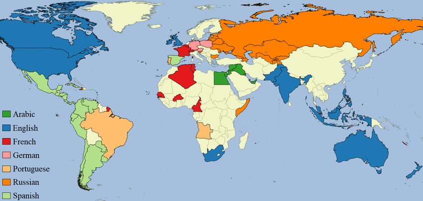
Dunn                                                                            Global Syntactic Variation

  What features do we use for dialectometry? Most previous work relies on phonetic or phonological
features (Kretzschmar, 1992, 1996; Heeringa, 2004; Labov et al., 2005; Nerbonne, 2006, 2009; Grieve et al.,
2011; Wieling and Nerbonne, 2011; Grieve, 2013; Nerbonne and Kretzschmar, 2013; Grieve et al., 2013;
Kretzschmar et al., 2014; Wieling and Nerbonne, 2015; Kruger and van Rooy, 2018) for the simple reason
that phonetic representations are relatively straight-forward: a vowel is a vowel and the measurements are
the same across varieties and languages. Previous work on syntactic variation has focused on either (i) an
incomplete set of language-specific variants, ranging from only a few features to hundreds (Sanders, 2007;
Szmrecsanyi, 2009; Sanders, 2010; Grieve, 2011; Collins, 2012; Grieve, 2012; Szmrecsanyi, 2013, 2014;
Grieve, 2016; Schilk and Schaub, 2016; Szmrecsanyi et al., 2016; Calle-Martin and Romero-Barranco,
2017; Grafmiller and Szmrecsanyi, 2018; Tamaredo, 2018) or (ii) language-independent representations
such as function words (Argamon and Koppel, 2013) or sequences of part-of-speech labels (Hirst and
Feiguina, 2007; Kroon et al., 2018). This forces a choice between either an ad hoc and incomplete syntactic
representation or a reproducible but indirect syntactic representation.

  This previous work on syntactic dialectometry has depended on the idea that a grammar is an inventory
of specific structures: the double-object construction versus the prepositional dative, for example. Under
this view, there is no language-independent feature set for syntax in the way that there is for phonetics. But
we can also view syntax from the perspective of a discovery-device grammar (Chomsky, 1957; Goldsmith,
2015): in this case, our theory of grammar is not a specific description of a language like English but rather
a function for mapping between observations of English and a lower-level grammatical description of
English: G = D(CORPUS). Thus, a discovery-device grammar (G) is an abstraction that represents what
the grammatical description would be if we applied the learner (D) to a specific sample of the language
(CORPUS). A discovery-device grammar allows us to generalize syntactic dialectometry: we are looking
for a model of syntactic variation, V , such that when applied to a grammar, V (G), the model is able to
predict regional variation in the grammar. But G is different for each language, so we generalize this to
V (D(CORPUS)). In other words, we use an independent corpus for each language as input to a discovery-
device grammar and then use the resulting grammar as a feature space for performing dialectometry. This
approach, then, produces an inventory of syntactic features for each language in a reproducible manner in
order to replace hand-crafted syntactic features. The specifics of the datasets used for modeling regional
variation are described in Section 2.1 and the discovery-device grammar used to create reproducible feature
sets is described in Section 2.2.
  What type of model should we use to represent global syntactic variation? Previous work has relied
largely on unsupervised methods like clustering (Wieling and Nerbonne, 2011), factor analysis of
spatial autocorrelation scores (Grieve, 2013), and individual differences scaling as an extension of
multidimensional scaling (Ruette and Speelman, 2014). These models attempt to aggregate individual
variants into larger bundles of features: which individual features represent robust aggregate isoglosses with
a similar geographic extent? The problem is that it is difficult to evaluate the predictions of one such bundle
against another. While useful for visualizations, these models are difficult to evaluate against ground-truths.
Another strand of work models the importance of predictor variables on the use of a particular variant,
with geographic region as one possible predictor (Szmrecsanyi et al., 2016). These models are based on
multivariate work in sociolinguistics that attempts to find which linguistic, social, or geographic features
are most predictive of a particular variant.
  While useful for understanding individual variants, however, these models are unable to handle the
aggregation of variants directly. For example, although it is possible to create a distance matrix between
regions for each individual feature and then to aggregate these matrices, the resulting aggregations are

This is a provisional file, not the final typeset article                                                    2
Dunn                                                                           Global Syntactic Variation

subject to variability: What is the best aggregation method? If two methods provide different maps, which
should we prefer? How stable are aggregations across folds? On the one hand, we want dialectometry to
establish a ground-truth about the regional distribution of variants and dialects. But, on the other hand,
because unsupervised methods like clustering are subject to such potential variability, we also need a
ground-truth to evaluate which aggregation method is the most accurate.
  One solution to this problem is to take a classification approach, in which the ground-truth is the region-
of-origin for individual samples. Given a model of dialectal variation, how accurately can that model
predict the region-of-origin of new samples? For example, the idea is that a more complete description of
the syntactic differences between Australian English and New Zealand English will be able to predict more
accurately whether a new sample comes from Australia or New Zealand. This prediction task provides a
ground-truth for aggregation. But it comes with two important caveats: First, a high prediction accuracy
does not guarantee that the model captures all relevant variation, only that it captures enough variation to
distinguish between national varieties. This can be mitigated, however, by using cross-fold validation and
unmasking as shown in Section 3.2. Second, while most work in dialectometry tries to establish geographic
boundaries, this work assumes geographic boundaries (i.e., polygons of nation-states).
  What languages and regions need to be represented in dialectometry? Because of coloniziation and
globalization (Kachru, 1990), a few languages like English are now used around the world by diverse
national communities. Even though these international languages have global speech communities,
dialectology and sociolinguistics continue to focus largely on sub-national dialects, often within so-
called inner-circle varieties (Kachru, 1982). This paper joins recent work in taking a global approach by
using geo-referenced texts (Goldhahn et al., 2012; Davies and Fuchs, 2015; Donoso and Sanchez, 2017) to
represent national varieties (Szmrecsanyi et al., 2016; Calle-Martin and Romero-Barranco, 2017; Cook and
Brinton, 2017; Rangel et al., 2017; Tamaredo, 2018; Dunn, 2018a, 2019b). The basic point is that in order to
represent regional variation as a complete system, dialectometry must take a global perspective. This paper
uses data-driven language mapping to choose (i) which international languages are used widely enough
to justify inclusion and (ii) which languages in which countries need to be included as national varieties.
We use geo-referenced corpora drawn from web pages and social media for both tasks. Seven languages
are selected for dialectometry experiments: Arabic, English, French, German, Portuguese, Russian, and
Spanish. These seven languages account for 59.25% of the web-crawled corpus and 74.67% of the social
media corpus. The corpora are regionalized to countries. Thus, the assumption is that any country which
frequently produces data in a language has a national variety of that language. For example, whether or not
there is a distinct variety of New Zealand English depends entirely on how much English data is observed
from New Zealand in these datasets. The models then have the task of determining how distinct New
Zealand English is from other national varieties of English.

  First, we consider the selection of (i) languages and (ii) national varieties of languages (Section 2.1)
as well as the selection of a syntactic feature space (Section 2.2). We then present the specifics of the
experimental framework (Section 2.3). Second, we compare prediction accuracies by language and feature
set (Section 3.1), in order to measure the quality of the models. Next, we evaluate the robustness of the
models across rounds of feature pruning and the similarity of the models across registers in order to examine
potential confounds (Section 3.2). Having validated the models themselves, the next section examines
regional accuracies and the similarities between national varieties (Section 3.3). Finally, we develop
measures for the syntactic uniqueness of each regional variety (Section 3.4) and search for empirical
correlates of concepts like inner-circle and outer-circle within this corpus-based approach (Section 3.5).
Third, we discuss two important issues: the application of different categorizations like inner-circle vs.

Frontiers                                                                                                  3
Dunn Global Syntactic Variation
Region Countries Population (%) Web (%) Twitter (%)
Africa, North 9 250 mil 3.4% 123.85 mil 0.7% 85.55 mil 2.1%
Africa, Southern 4 75 mil 1.0% 59.07 mil 0.4% 87.34 mil 2.1%
Africa, Sub-Saharan 73 742 mil 10.1% 424.75 mil 2.6% 254.20 mil 6.1%
America, Brazil 1 206 mil 2.8% 218.11 mil 1.3% 118.13 mil 2.9%
America, Central 25 214 mil 2.9% 886.61 mil 5.3% 383.81 mil 9.3%
America, North 2 355 mil 4.8% 236.59 mil 1.4% 350.12 mil 8.5%
America, South 11 210 mil 2.9% 1,163.00 mil 7.0% 402.15 mil 9.7%
Asia, Central 10 198 mil 2.7% 965.09 mil 5.8% 102.79 mil 2.5%
Asia, East 8 1,635 mil 22.3% 2,201.86 mil 13.2% 95.70 mil 2.3%
Asia, South 7 1,709 mil 23.3% 448.23 mil 2.7% 331.19 mil 8.0%
Asia, Southeast 22 615 mil 8.4% 2,011.06 mil 12.1% 245.18 mil 5.9%
Europe, East 17 176 mil 2.4% 4,553.10 mil 27.4% 322.46 mil 7.8%
Europe, Russia 1 144 mil 2.0% 101.44 mil 0.6% 105.04 mil 2.5%
Europe, West 25 421 mil 5.7% 2,422.85 mil 14.6% 823.80 mil 19.9%
Middle East 15 334 mil 4.5% 660.73 mil 4.0% 222.98 mil 5.4%
Oceania 8 59 mil 1.0% 164.02 mil 1.0% 213.06 mil 5.1%
TOTAL 199 7.35 bil 100% 16.65 bil 100% 4.14 bil 100%
Table 1. Size of Geo-Referenced Corpora in Words by Region
outer-circle or native vs. non-native to these datasets (Section 4.1) and the implications of a computational
approach to dialectometry for sociolinguistics more broadly (Section 4.2).
2 MATERIALS AND METHODS
2.1 Language Mapping and Dialectometry
We begin with data-driven language mapping: First, what languages have enough national varieties to
justify modeling? Second, which national varieties should be included for each language? Third, which
datasets can be used to represent specific national varieties and how well do these datasets represent the
underlying populations? This paper depends on geo-referenced corpora: text datasets with meta-data that
ties each document to a specific place. The size of both datasets by region is shown in Table 1, together
with ground-truth population data from the UN (United Nations, 2017). The size of each region relative
to the entire dataset is also shown: for example, 14.6% of the web corpus comes from Western Europe
which accounts for only 5.7% of the global population. This comparison reveals the over-representation
and under-representation of each region.
Data comes from two sources of digital texts: web pages from the Common Crawl1 and social media
from Twitter2 . The Common Crawl data represents a large snapshot of the internet; although we cannot
direct the crawling procedures, we are able to process the archived web pages from the perspective of
1 http://www.commoncrawl.org
2 http://www.twitter.com
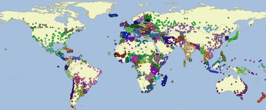
This is a provisional file, not the final typeset article 4Dunn Global Syntactic Variation Figure 1. Cities for Collection of Twitter Data (50km radius from each) a geo-referenced corpus. The author of each individual web page may be unknowable but we can use country-specific top-level domains for country-level geo-referencing: for example, web pages under the .nz domain are from New Zealand. Previous work has shown that there is a relationship between domain-level geo-referenced web pages and national varieties (Cook and Brinton, 2017). Some countries are not available because their top-level domains are used for other purposes (i.e., .ai, .fm, .io, .ly, .ag, .tv). Domains that do not contain geographic information are also removed from consideration (e.g., .com sites). The Common Crawl dataset covers 2014 through the end of 2017, totalling 81.5 billion web pages. As shown in Table 1, after processing this produces a corpus of 16.65 billion words. This dataset represents 166 out of 199 total countries considered in this paper. Some countries do not use their country-level domains as extensively as others: in other words, .us does not account for the same proportion of web pages from the United States as .nz does from New Zealand. It is possible that this skews the representation of particular areas. Thus, Table 1 shows the UN-estimated population for each region as reference. The web corpus is available for download3 as is the code used to create the corpus.4 In isolation, web-crawled data provides one observation of global language use. Another common source of data used for this purpose is Twitter (e.g., Eisenstein, et al., 2010; Roller, et al., 2012; Kondor, et al., 2013; Mocanu, et al., 2013; Eisenstein, et al., 2014; Graham, et al., 2014; Donoso & Sanchez, 2017). The shared task at PAN-17, for example, used Twitter data to represent national varieties of several languages (Rangel et al., 2017). A spatial search is used to collect Tweets from within a 50km radius of 10k cities.5 This city-based search avoids biasing the selection by using language-specific keywords or hashtags. A map of each city used for collection is shown in Figure 1; while this approach avoids a language-bias, it could under-represent rural areas given the 50 km radius of each collection area. The Twitter data covers the period from May of 2017 until early 2019, drawn from the Twitter API using a spatial query. This creates a corpus containing 1,066,038,000 Tweets. The language identification component, however, only provides 3 https://labbcat.canterbury.ac.nz/download/?jonathandunn/CGLU_v3 4 https://github.com/jonathandunn/common_crawl_corpus 5 https://github.com/datasets/world-cities Frontiers 5
Dunn                                                                               Global Syntactic Variation

reliable predictions for samples containing at least 50 characters (c.f., the language id code6 and the models
used7 ). Thus, the corpus is pruned to include only Tweets above that length threshold. As shown in Table 1,
this produces a corpus containing 4.14 billion words. While the Common Crawl corpus represents 166
countries, the Twitter corpus represents 169. There are 33 countries that only Twitter represents (not the
Common Crawl) and 30 that only the Common Crawl represents (not Twitter). This shows the importance
of drawing on two different sources of language use.
  Given the idiosyncracies of these two datasets (i.e., the availability of country-codes for web data and the
selection of cities for Twitter data), it is quite likely that each represents different populations or, at least,
that each represents different registers of language usage from the same population. We can use ground-
truth population data to deal with the problem of different populations. First, notice that both datasets
under-represent all regions in Africa; but the web dataset has the worst under-representation: while Africa
accounts for 14.5% of the world’s population, it accounts for only 3.7% of the web corpus. The Americas
and Europe, on the other hand, are over-represented in both datasets. Twitter especially over-represents
North America (8.5% of the corpus vs. 4.8% of the population); but the web corpus under-represents North
America (only 1.4% of the corpus), mostly from the lack of adoption of the .us domain. Western Europe
is over-represented in both corpora: while it acounts for only 5.7% of the population, it provides 14.6%
of the web corpus and 19.9% of the Twitter corpus. Although these trends are expected, it is helpful to
quantify the degree of over-representation. Less expectedly, the web corpus greatly over-represents Eastern
Europe (27.4% of the corpus but only 2.4% of the population). Asia, especially the East and South, are
under-represented in both datasets.
  On the one hand, the use of population data here allows us to quantify exactly how each of these datasets
is skewed. On the other hand, our purpose is to model regional syntactic variation: do the datasets need
to be prefectly aligned with regional populations in order to achieve this? There are two observations to
be made: First, if a region is over-represented then we do not need to worry about missing any national
varieties from that area; but we should be worried about over-representing those particular national varieties
(this is why there is a cap on the number of training samples from each dialect). Second, it could be the
case that we are missing national varieties from under-represented areas. For example, any missing national
varieties are likely to be from Africa or East Asia, given the skewed representations of this dataset. Related
work, however, has shown that it in the case of major international languages like those considered here,
the problem is over-representation rather than under-representation in the form of missing regional varieties
(Dunn, 2019a). We leave it to future work to make improvements in the selection of regional varieties using
population-based sampling to overcome skewness in corpus distributions.
  What languages should be included in a model of global syntactic variation? Given that we are using
countries to define regional varieties, a language needs to occur in many countries. Here we use a threshold
of 1 million words to say that a language is used significantly in a given country. Table 2 shows the seven
languages included in this study, encompassing 59.25% of the web corpus and 74.67% of the Twitter
corpus. Some other languages occur in several countries in one dataset but not the other and so are not
included. For example, Italian occurs in 17 countries in the web corpus but only 2 in the Twitter corpus;
Indonesian occurs in 10 countries in the web corpus but only 3 countries in the Twitter corpus. Given that
we model varieties using a classifier, we focus on those languages that have a sufficient number of national
varieties to make classification a meaningful approach.

6   https://github.com/jonathandunn/idNet
7   https://labbcat.canterbury.ac.nz/download/?jonathandunn/idNet_models

This is a provisional file, not the final typeset article                                                       6
Dunn                                                                             Global Syntactic Variation

2.2 Finding Syntactic Variants
  This paper represents syntactic variants using a discovery-device Construction Grammar (CxG) that
produces a CxG for each language given an independent corpus representing that language. CxG itself is a
usage-based paradigm that views grammar as a set of overlapping constructions made up of slot-fillers
defined by syntactic, semantic, and sometimes lexical constraints (Goldberg, 2006; Langacker, 2008). This
paper draws on recent approaches to computational modeling of CxGs (Dunn, 2017, 2018b; Dunn and
Adams, 2019), including previous applications of a discovery-device CxG to dialectometry for English
(Dunn, 2018a, 2019b).
  Constructions are represented as a sequence of slot-constraints, as in (1a). Slots are separated by dashes
and constraints are defined by both type (Syntactic, Joint Semantic-Syntactic, Lexical) and by filler (for
example: NOUN, a part-of-speech or ANIMATE, a semantic domain).
(1a) [SYN:NOUN — SEM-SYN:TRANSFER [V] — SEM-SYN:ANIMATE [N] — SYN:NOUN]
(1b) “He gave Bill coffee.”
(1c) “He gave Bill trouble.”
(1d) “Bill sent him letters.”
(2a) [SYN:NOUN — LEX:“give” — SEM-SYN:ANIMATE [N] — LEX:“a hand”]
(2b) “Bill gave me a hand.”

  The construction in (1a) contains four slots: two with joint semantic-syntactic constraints and two
with simple syntactic constraints. The examples in (1b) to (1d) are tokens of the construction in (1a).
Lexical constraints, as in (2a), represent idiomatic sentences like (2b). A CxG is a collection of many
individual constructions. For the purposes of dialectometry, these are quantified as one-hot encodings
of construction frequencies. This, in essence, provides a bag-of-constructions that is evaluated against
traditional bag-of-words features.
  A large portion of the language-learning corpus for each language comes from web-crawled data (Baroni
et al., 2009; Majliˇs and ZdenˇekˇZabokrtsky, 2012; Benko, 2014) and data from the CoNLL 2017
Shared Task (Ginter et al., 2017). Because the goal is to provide a wide representation of each language,
this is augmented by legislative texts from the EU and UN (Tiedemann, 2012; Skadiņš et al., 2014), the
OpenSubtitles corpus (Tiedemann, 2012), and newspaper texts. The exact collection of documents used for
learning CxGs is available for download.8 While both web-crawled and social media datasets are used to
represent national varieties, the grammars used are learned mainly from web-crawled corpora. On the one
hand, we use separate datasets for grammar learning and dialectometry in order to remove the possible
confound that the grammars are over-fitting a specific dataset. On the other hand, we do not explicitly know
which regional varieties the data used for grammar learning is drawn from. The discussion in Section 3.5,
as well as other work (Dunn, 2019b), shows that at least the English grammar better represents inner-circle
varieties like UK English. In this case, then, we prefer to avoid the possible confound of over-fitting even
though the result is a grammar that is learned from datasets implicitly drawn from inner-circle varieties.
  This paper evaluates two alternate CxGs for dialectometry, alongside function words and lexical features:
CxG-1 (Dunn, 2018b,a) and CxG-2 (Dunn and Adams, 2019). As described and evaluated elsewhere (Dunn
and Adams, 2019), CxG-1 relies on frequency to select candidate slot-constraints while CxG-2 relies
on an association-based search algorithm. The differences between the two competing discovery-device
grammars as implementations of different theories of language learning are not relevant here. Rather,

8   https://labbcat.canterbury.ac.nz/download/?jonathandunn/CxG_Data_FixedSize

Frontiers                                                                                                 7
Dunn                                                                             Global Syntactic Variation

we evaluate both grammars because previous work (Dunn, 2018a) relied on CxG-1 and this comparison
makes it possible to connect the multi-lingual experiments in this paper with English-only experiments in
previous work. It should be noted, however, that other work has shown that association-based constraints
out-perform frequency-based constraints across several languages (Dunn and Adams, 2019). As shown in
Section 3, this paper finds that association-based constraints also perform better on the task of dialectometry.
This is important because the evaluation connects the emergence of syntactic structure with variation in
syntactic structure.
  Previous work on syntactic dialectometry focuses on paired sets of features which can be viewed as
alternate choices that express the same function or meaning. In other words, these approaches contrast
constructions like the double object vs. the prepositional dative and then quantify the relative preference of
particular varieties for one variant over the other. From our perspective, such an approach is essential for a
limited feature space because syntactic variation is structured around different constructions that encode
the same function or meaning. In other words, two constructions which have entirely different uses cannot
be in competition with one another: constrasting the double object and the get-passive constructions, in
isolation, is not a meaningful approach to syntactic variation because their frequencies are influenced by
other unseen parts of the grammar. On the other hand, looking at the frequency of a single construction in
isolation can be meaningful but will never reveal the full picture of syntactic variation.
  This whole-grammar construction-based approach to dialectology represents as much of the functional
space as possible. This provides an implicit pairing of syntactic variants: without a topic bias, we expect that
the relative frequency of a specific construction will be consistent across documents. If one construction
is more frequent, that indicates an increased preference for that construction. This approach does not
explicitly pair variants because part of the problem is to learn which constructions are in alternation. From a
different perspective, we could view alternating variants as knowledge that is traditionally given to models
within quantitative sociolinguistics: which constructions are in competition with one another? But the idea
here is to leave it to the model itself to determine which constructions are in competition.
  Because this work is situated within both dialectometry and construction grammar, we view syntactic
variation as fundamentally structured around function and meaning (as described above). But more
traditional sociolinguistic and generativist work on syntactic variation does not share this underlying view.
In this case the prediction task itself allows us to translate between competing assumptions: regardless of
how we understand the source of variation, the models are ultimately evaluated on how well they are able
to predict region-of-origin (samples from New Zealand vs. samples from Australia) using only syntactic
representations. This type of ground-truth evaluation can be undertaken, with greater or lesser success,
with any set of assumptions. Whether or not dialectal variation is fundamentally based on alternations and
whether or not dialectometry models require alternations, the argument here is that the ability to distinguish
between dialects (without topic-based features) is a rigorous evaluation of the quality of a model of dialects.
  Finally, how does geographic variation as modeled here interact with register variation? We can think
about this in two different ways: First, does register variation within these datasets present a confound
by being structured geographically? In other words, if the corpus from Australia represents newspaper
and magazine articles but the corpus from New Zealand represents discussion forums, then the ability
to distinguish between the two is a confound. Given the size of the datasets, the consistent collection
methodology, the cross-fold validation experiments, the large number of national varieties per language,
and the comparison of web-based and Twitter data, however, this confound is not likely. Second, is register
variation the same underlying phenomenon as regional variation? In other words, is the difference between
New Zealand English and Australian English ultimately the same type of phenomenon as the structured

This is a provisional file, not the final typeset article                                                     8
Dunn                                                                                                                     Global Syntactic Variation

       Language                      Countries (Web)                 Words (Web)               Countries (Twitter)                  Words (Twitter)
       Arabic (ara)                              19                     348,671,000                          25                            179,473,000
       English (eng)                            130                  4,990,519,000                          137                         1,552,268,000
       French (fra)                              36                     479,857,000                          24                            176,009,000
       German (deu)                              24                     500,029,000                           7                             71,234,000
       Portuguese (por)                          14                     431,884,000                          22                            199,080,000
       Russian (rus)                             37                  1,361,331,000                            9                            126,834,000
       Spanish (spa)                             43                  1,757,200,000                           44                            789,239,000
                                          % of Total:                          59.25%                 % of Total:                                 74.67%
       Language                       Varieties (Web)               N. Test (Web)               Varieties (Twitter)                N. Test (Twitter)
       Arabic (ara)                               4                             14,685                        7                                     15,537
       English (eng)                             14                             66,476                       14                                     64,208
       French (fra)                              13                             46,562                        4                                     12,130
       German (deu)                               7                             35,240                        2                                      7,722
       Portuguese (por)                           4                             15,129                        2                                       8,650
       Russian (rus)                             19                             84,925                        3                                       9,164
       Spanish (spa)                             17                             84,093                       17                                     76,653

Table 2. Above: Number of Countries and Words by Language and Domain
Below: Number of Varieties and Test Samples by Language and Domain

difference between newspaper writing and discussion forums? This is an empirical question for future
work that requires a dataset containing both register meta-data and spatial meta-data.
2.3 Modeling National Varieties
  The experiments in this paper take a classification approach to dialectometry: given a one-hot encoding
of construction frequencies (i.e., a bag-of-constructions), can we distinguish between different national
varieties of a language? There are two main advantages to this approach: First, the model can be evaluated
using prediction accuracies on held-out testing data. This is important to ensure that the final model is
meaningful. Second, a classification approach provides an implicit measure of the degree of syntactic
separation between national varieties across the entire grammar (c.f., region similarities in Section 3.3). A
particular construction may be unique to a given variety, but this in itself is less meaningful if the varieties
are otherwise the same. How deep or robust is the syntactic variation? How distinct are the national
varieties? Dialectometry is about going beyond variation in individual syntactic features to measure the
aggregate syntactic relationships between varieties.
  The main set of experiments uses a Linear Support Vector Machine (Joachims, 1998) to classify varieties
using CxG features. Parameters are tuned using separate development data.9 Given the general robust
performance of SVMs in the literature relative to other similar classifiers on latent variation tasks (Dunn
et al., 2016), we forego a systematic evaluation of classifiers. For reproducibility against future work, all
results are calculated on pre-specified training and testing sets. Given the large number of samples in each
test set (Table 2) and the robustness in the cross-validation evaluation (Table 4) we are not concerned with

9   Development data allows experimental settings and parameters to be evaluated without over-fitting the training/testing data that is used for the main experiment.

Frontiers                                                                                                                                                          9
Dunn Global Syntactic Variation over-fitting and given the high performance in general we are not concerned with under-fitting (Table 3). Under this evaluation regime, any classifier could be used; thus, it is not important to contrast a Linear SVM with other shallow classifiers such as Naive Bayes or Decision Trees in this context. The Linear SVM uses the training data to learn weights for each construction in the grammar for each regional variety; in the aggregate, the model builds a high-dimensional representation of each variety that maximizes the distance between them (i.e., so that varieties like American English and Nigerian English can be easily separated). The quality and generalizability of the models are evaluated using held-out testing data: how well can those same feature weights be used to predict which regional variety a new sample belongs to? Because it is possible here that the varieties could be distinguished in a low-dimensional space (i.e., being separated along only a few constructions), we use unmasking to evaluate the robustness of the models in Section 3.2. This classification-based approach deals very well with the aggregation of features, including being able to ignore redundant or correlated features. On the other hand, this robust aggregation of syntactic features requires that we assume the spatial boundaries of each regional variety. Moving to data preparation, the assumption is that a language sample from a web-site under the .ca domain originated from Canada. This approach to regionalization does not assume that whoever produced that language sample was born in Canada or represents a traditional Canadian dialect group; rather, the assumption is only that the sample represents someone in Canada who is producing language data; but the two are closely related (Cook and Brinton, 2017). This corresponds with the assumption that Twitter posts geo-referenced to particular coordinates represent language use in that place but do not necessarily represent language use by locals. Geo-referenced documents represent language use in a particular place. Unlike traditional dialect surveys, however, there is no assurance that individual authors are native speakers from that place. We have to assume that most language samples from a given country represent the native varieties of that country. For example, many non-local residents live in Australia; we only have to assume that most speakers observed in Australia are locals. On the one hand, this reflects the difference between corpus-based and survey-based research: we know less about the individuals who are represented in these datasets. On the other hand, this reflects increased mobility: the idea that a local individual is born, is raised, and finally dies all in the same location is no longer proto-typical. In order to average out the influence of out-of-place samples, we use random aggregation to create samples of exactly 1,000 words in both corpora. For example, in the Twitter corpus this means that an average of 59 individual Tweets from a place are combined into a single sample. First, this has the effect of providing more constructions per sample, making the modelling task more approachable. Second and more importantly, individual out-of-place Tweets and web pages are reduced in importance because they are aggregated with other Tweets and web pages presumably produced by local speakers. If we think of non-locals as outliers, this approach aggregates outliers with non-outliers in order to reduce their influence. We leave for future work an evaluation of different approaches to this problem. The larger issue is the relationship between small but carefully curated corpora for which significant meta-data is available for each speaker and these large but noisy corpora which are known to contain out-of-place samples (i.e., tourists in Twitter data). One promising approach is to evaluate such noisy corpora based on how well they are able to predict demographic meta-data for the places they are intended to represent (Dunn, 2019a). In this case, it has been shown that web-crawled and Twitter corpora are significantly correlated with population density (especially when controlling for GDP and general rates of internet usage) and that both datasets can be used to predict which languages are used in a country (as represented using census data). While there is much work to be done on this problem, the prediction of demographic meta-data provides a way to evaluate the degree to which large and noisy corpora reflect actual populations. This is a provisional file, not the final typeset article 10
Dunn                                                                            Global Syntactic Variation

Figure 2. Countries with National Varieties for Selected Languages

  We take a simple threshold-based approach to the problem of selecting national varieties to include. For
English and Spanish, any national variety that has at least 15 million words in both the Common Crawl and
Twitter datasets is included. Given the large number of countries in Table 2, this higher threshold accounts
for the fact that both English and Spanish are widely used in these datasets. Lower relative thresholds are
used for the other languages, reflecting the more limited prevalence of these languages: the thresholds are
made relative to the amount of data per language and are comparable to the English and Spanish threshold.
For English and Spanish, the national varieties align across both datasets; thus, the experiments for these
two languages are paired and we also consider similarity of models across registers. But for the other
languages aligning the national varieties in this way removes too many from consideration; thus, there is
no cross-domain evaluation for Arabic, French, German, Portuguese, or Russian.

  The inventory of national varieties in Table 2 is entirely data-driven and does not depend on distinctions
like dialects vs. varieties, inner-circle vs. outer-circle, or native vs. non-native. Instead, the selection is
empirical: any area with a large amount of observed English usage is assumed to represent a national
variety of English. Since the regions here are based on national boundaries, we call these national varieties.
We could just as easily call them national dialects or regional varieties. The global distribution of national
varieties for each language is shown in Figure 2.

  The datasets are formed into training, testing, and development sets as follows: First, 2k samples are used
for development purposes regardless of the amount of data from a given variety. Depending on the size
of each variety, at least 12k training and 2.5k testing samples are available. Because some varieties are
represented by much larger corpora (i.e., Tweets from American English), a maximum of 25k training
samples and 5k testing samples are allowed per variety per register. These datasets contain significantly
more observations than have been used in previous work (Dunn, 2018a).

Frontiers                                                                                                  11
Dunn                                                                              Global Syntactic Variation

  For each language, we compare six sets of features: First, syntactic representations using CxG-1 and
CxG-2; Second, indirect syntactic representations using function words10 ; Third, unigrams and bigrams
and trigrams of lexical items. Lexical unigrams represent mostly non-syntactic information while increasing
the size of n begins to indirectly include information about transitions. The n-grams are representing using
a hashing vectorizer with 30k dimensions (thus, these representations have no syntactic features present).
This avoids biasing the selection of specific n-grams (i.e., with content more associated with dominant
inner-circle varieties). But this also means that the lexical features themselves cannot be inspected.

3      RESULTS
This section reports the results of dialectometry experiments across seven languages. First, in Section
3.1 we look at overall predictive accuracy using the F-Measure metric across feature sets and languages.
The purpose of this analysis is to contextualize and then explore the interpretation of classification-based
dialectometry. Second, in Section 3.2 we examine the robustness of models across registers (using the
web corpus and the Twitter corpus) and across rounds of feature pruning. The purpose of this analysis is
to understand how meaningful these models are in the presence of possible confounds such as a reliance
on a small number of highly predictive variants. These first two sections are important for validating a
classification-based approach to syntactic variation. Third, in Section 3.3 we analyze predictive accuracy
and prediction errors across languages and develop representations of regional syntactic similarity. The
purpose of this analysis is to use dialect classification to understand global syntactic variation in the
aggregate. Fourth, in Section 3.4 we examine measures of the uniqueness of different regional varieties
and in Section 3.5 we apply these models to evaluate empirical correlates for notions like inner-circle and
outer-circle. These last two sections are important for understanding what dialect classification can tell us
about global, whole-grammar syntactic variation once the approach itself has been validated.
3.1 Features, Model Size, and Predictive Accuracy
  The overall prediction accuracy across languages is shown in Table 3 (with the web corpus above and the
Twitter corpus below). On the left-hand part of the table, the syntactic features are grouped: function words
and the two CxG feature sets. On the right-hand part, the lexical features are grouped: lexical unigrams,
bigrams, and trigrams. For reference, the number of regions for each variety is shown in the final column.
  A classification-based approach has the goal of distinguishing between national varieties. We would
expect, then, that the task of distinguishing between a small number of varieties is easier than distinguishing
between a larger number of varieties. For example, there are only two varieties of German and Portuguese
in the Twitter corpus. For Portuguese, all feature sets have F1s of 1.00 or 0.99; in other words, this is an easy
task and there are many ways of doing it. This is also an indication that these varieties of Portuguese (here,
from Brazil, BR, and from Portugal, PT) are quite distinct across all feature sets. On the other hand, even
though German also has a small number of national varieties (here, from Germany, DE, and from Austria,
AT), there is a wide variation in prediction accuracy, with function words (F1 = 0.83) and CxG-1 (F1 =
0.90) having markedly lower performance than other feature sets. The point is that model performance
depends on both the number of national varieties included in the model (showing the importance of taking
an empirical approach to the selection of varieties) as well as on the degree of difference between the
varieties themselves. Portuguese as used in Brazil and Portugal is significantly more distinct than German
as used in Germany and Austria. Digging deeper, however, we also notice that function words as features
are more uneven across languages than other feature sets. For example, Arabic on Twitter has eight national
varieties and function words achieve an F1 of 0.80; but for Russian on Twitter, with only three varieties,

10   For replicability, these are taken from https://github.com/stopwords-iso

This is a provisional file, not the final typeset article                                                    12
Dunn                                                                              Global Syntactic Variation

function words achieve a lower F1 of 0.73. This is an indication that, as indirect proxies for syntactic
structure, the usefulness of function words for this task varies widely by language (at least, given the
inventory of function words used here).
  Regardless of the number of national varieties per language, lexical unigrams perform the best (F1 = 1.00).
In other words, it is not difficult to disinguish between samples from New Zealand and Australia when given
access to lexical items (Christchurch vs. Brisbane). While we know that syntactic models are capturing
linguistic variation, however, the success of lexical models, as argued elsewhere (Dunn, 2019b), is partly a
result of place-names, place-specific content, and place-specific entities. In other words, geo-referenced
texts capture the human geography of particular places and this human geography information takes the
form of specific lexical items. Previous work has focused on capturing precisely this type of content (Wing
and Baldridge, 2014; Hulden et al., 2015; Adams, 2015; Lourentzou et al., 2017; Adams and McKenzie,
2018). The problem is that, without organizing the frequency of such lexical features according to concept
(Zenner et al., 2012), these models may not represent linguistic variation.
  This is a simplification, of course, but the underlying point is that it is difficult to distinguish linguistic
lexical variation from human geography-based and topical lexical variation without relying on the idea of
conceptual alternations. For example, we know that as n increases n-grams represent increasing structural
information (i.e., transitions between lexical items instead of lexical items in isolation). Here we see that,
by the time n is raised to three, the predictive accuracy of CxG-2 always surpasses the predictive accuracy
of trigrams (with the single exception of French on Twitter). The difference between CxG-2 and bigrams is
much smaller than the distance between the various syntactic features. This is evidence that the advantage
of unigrams over CxG-2 reflects the advantage of human geography content (i.e., lexical items in isolation)

     CC             Function CxG-1           CxG-2       Unigram Bigram Trigram               N. Regions
     Arabic            0.88        0.90         1.00        1.00        1.00        0.96            4
     English           0.65        0.80         0.96        1.00        0.98        0.87           14
     French            0.61        0.78         0.96        1.00        0.98        0.90           13
     German            0.84        0.89         0.96        1.00        0.98        0.86            8
     Portuguese        0.89        0.98         0.99        1.00        1.00        0.97            4
     Russian           0.41        0.79         0.95        1.00        0.95        0.80           19
     Spanish           0.52        0.78         0.95        1.00        0.99        0.91           17
     TW             Function CxG-1           CxG-2       Unigram Bigram Trigram               N. Regions
     Arabic            0.80        0.88         0.98        1.00        1.00        0.94            8
     English           0.55        0.76         0.92        1.00        0.97        0.82           14
     French            0.88        0.98         0.98        1.00        1.00        0.99            4
     German            0.83        0.90         0.95        1.00        0.99        0.95            2
     Portuguese        1.00        0.99         1.00        1.00        1.00        0.99            2
     Russian           0.73        0.83         0.93        1.00        0.94        0.87            3
     Spanish           0.51        0.82         0.94        1.00        0.99        0.92           17

Table 3. F1 of Classification of Regional Varieties by Language and Feature Type
(Web Corpus Above and Twitter Corpus Below)

Frontiers                                                                                                    13
Dunn Global Syntactic Variation over linguistic variation (i.e., transitions between lexical items). In short, while some of the lexical variation is linguistic (soda vs. pop), a good deal of it is also based on human geography (Chicago vs. Singapore). The advantage of syntactic models in this context is that such non-linguistic variations do not introduce confounds: we know that these models represent regional varieties of each language. Models on the web corpus (above) have higher predictive accuracy than models on the Twitter corpus (below). This is true except in cases, such as Portuguese, where there is a wide difference in the number of national varieties represented (for Portuguese, two vs. four). For reasons of data availability, only English and Spanish have strictly aligned varieties; in both of these languages, the syntactic features perform better on the web corpus than the Twitter corpus, although the gap is wider for English than for Spanish. This raises a question that is addressed in the next section: are models of syntactic variation consistent across these registers? In other words, do the web-based and Twitter-based models make the same types of errors? The web corpus also provides more varieties per language (with Arabic as the sole exception, which is better represented on Twitter). In many cases this difference is significant: there are 19 varieties of Russian on the web, but only three on Twitter. In this case, there are competing Russian-language social media platforms (i.e., www.vk.com) that are not included in this study. In other words, outside of English and Spanish, which are aligned across datasets, the Twitter data is less comprehensive. What does the F-Measure tell us about models of syntactic variation? First, the measure is a combination of precision and recall that reflects the predictive accuracy while taking potentially imbalanced classes into account: how many held-out samples can be correctly assigned to their actual region-of-origin? On the one hand, this is a more rigorous evaluation than simply finding a significant difference in a syntactic feature across varieties within a single-fold experimental design: not only is there a difference in the usage of a specific feature, but we can use the features in the aggregate to characterize the difference between national varieties. On the other hand, it is possible that a classifier is over-fitting the training data so that the final model inflates the difference between varieties. For example, let’s assume that there is a construction that is used somewhat frequently in Pakistan English but is never used in other varieties. In this case, the classifier could achieve a very high prediction accuracy while only a single construction is actually in variation. Before we interpret these models further, the next section evaluates whether this sort of confound is taking place. 3.2 Model Robustness Across Features and Registers If a classification model depends on a small number of highly predictive features, thus creating a confound for dialectometry, the predictive accuracy of that model will fall abruptly as such features are removed (Koppel et al., 2007). Within authorship verification, unmasking is used to evaluate the robustness of a text classifier: First, a linear classifier is used to separate documents; here, a Linear SVM is used to classify national varieties of a language. Second, for each round of classification, the features that are most predictive are removed: here, the highest positive and negative features for each national variety are pruned from the model. Third, the classifier is retrained without these features and the change in predictive accuracy is measured: here, unmasking is run for 100 iterations using the CxG-2 grammar as features, as shown in Figure 3 (with the web-based model above and the Twitter-based model below). For example, this removes 28 constructions from the model of English each iteration (two for each national dialect), for a total of approximately 2,800 features removed. The figures show the F-Measure for each iteration. On the left-hand side, this represents the performance of the models with all features are present; on the right-hand side, this represents the performance of the models after many features have been removed. This provides a measure of the degree to which these models are subject to a few highly predictive features. This is a provisional file, not the final typeset article 14
Dunn                                                                  Global Syntactic Variation

                                              Web

       1

   0.95

    0.9

   0.85

    0.8

   0.75
            13

            28

            52

            67

            76

            91
            10

            16
            19
            22
            25

            31
            34
            37
            40
            43
            46
            49

            55
            58
            61
            64

            70
            73

            79
            82
            85
            88

            94
            97
             1
             4
             7

           100
            Arabic    English     French     German     Portuguese     Russian     Spanish

                                            Twitter

       1

   0.95

    0.9

   0.85

    0.8

   0.75
            13

            22

            31

            40

            49

            58

            67

            76

            85

            94
            10

            16
            19

            25
            28

            34
            37

            43
            46

            52
            55

            61
            64

            70
            73

            79
            82

            88
            91

            97
             4
             1

             7

           100

            Arabic    English     French     German      Portuguese    Russian     Spanish

Figure 3. Model Robustness by Language Using Unmasking for 100 Iterations with CxG-2 Features
(Web Models Above and Twitter Models Below)

Frontiers                                                                                       15
Dunn Global Syntactic Variation First, we notice that models with a higher starting predictive accuracy (e.g., Arabic and Portuguese in the web-based model and Portuguese and French in the Twitter-based model) tend to maintain their accuracy across the experiment. Even after 100 rounds of pruning, Arabic and Portuguese (CC) remain above 0.95 with CxG-2 features.11 Similarly, French and Portuguese remain above 0.95 after 100 rounds of pruning (TW). This indicates that a high performing dialect classification model is based on a broad and distributed set of features. But this is not always the case: for example, Arabic (TW) starts out with the same performance as French but over the course of the experiment declines to a performance that is 10% lower than French. This is an indication that this Twitter-based model of Arabic is less robust than its counter-part model of French (although keep in mind that the French model has only 4 varieties and the Arabic model has 8). Second, although Spanish and Russian have a starting accuracy that is comparable to other languages, with F1s of 0.95 for both languages on the web corpus, their accuracy falls much more quickly. Spanish and Russian decrease by around 20% by the end of the experiment while English and French decrease by only 10% in total. On the Twitter corpus, Spanish and Russian again pattern together, this time with a 15% reduction. But here the English model has a somewhat steeper decline. In most cases, however, the starting accuracy of a model is related to its rate of decline: more accurate models are also more robust to feature pruning. The purpose of this evaluation is to show that a classification approach to dialectometry is not subject to the confound of a small number of highly predictive features. The next question is about the similarity of national varieties as represented in the web corpus vs. the Twitter corpus. Is there a consistent representation of variation or are the models ultimately register-specific? For this analysis we focus on English and Spanish as the two languages that are aligned by national varieties across both datasets. We focus on an analysis of errors: First, two national varieties that are more often confused by the classifier are more similar according to the model. Thus, we represent the similarity of regions using the total of all errors between two varieties. For example, if UK English is predicted to be New Zealand English 50 times and New Zealand English is predicted to be UK English 25 times, there are 75 total errors between these varieties. More errors reflects more similar varieties.12 The question is whether the web corpus and Twitter both provide the same patterns of similarity. Figure 4 shows the relative errors between varieties for both datasets (with English above and Spanish below): the web (blue) occupies the left-hand side of each bar and Twitter (red) occupies the right-hand side. If both colors are the same size, we see the same proportion of errors for a given pair across both datasets. This figure also shows the most similar varieties, with the varieties having the highest total errors occupying the bottom of each. For example, the most similar varieties of English on Twitter are American (US) and Canadian English (CA). The most similar varieties on the web corpus, however, are New Zealand (NZ) and South African English (ZA).13 The Pearson correlation between errors, paired across datasets by varieties, is highly significant for English at 0.494 (note that this involves the number of errors but does not require that the errors themselves match up across registers). At the same time, there remain meaningful differences between the datasets. For example, Nigeria (NG) and Portugal (PT) have many errors in the Twitter model but very few in the web model. On the other hand, New Zealand (NZ) and South Africa (ZA) have a large number of errors in the web model but few in the Twitter model. This is an indication that the models are somewhat different across registers. 11 Here and below we focus on CxG-2 as the highest performing syntactic model. 12 Country abbreviations are given in Appendix A. 13 The ISO country codes are used in all figures and tables; these are shown by common name in the first Appendix. This is a provisional file, not the final typeset article 16
Dunn                                                                        Global Syntactic Variation

                                               English

        PT & US
        AU & IE
       NZ & US
       MY & NZ
       NG & ZA
       CA & ZA
       AU & ZA
       NZ & UK
                                                                                     Web
       US & ZA
       CA & NZ                                                                       Twitter
        IN & PK
        IE & UK
       NZ & ZA
       AU & UK
       AU & US
       CA & UK
       NG & PT
       AU & NZ
       AU & CA
       CA & US
                  0    0.1     0.2     0.3     0.4    0.5     0.6     0.7      0.8    0.9      1

                                              Spanish

       PE & UY
       CO & VE
       HN & SV
       MX & VE
       GT & HN
        PA & SV
       GT & MX
        GT & NI
                                                                                     Web
       CU & VE
        NI & SV                                                                      Twitter
        ES & VE
       GT & SV
       ES & MX
       PY & UY
       AR & PY
       CR & PY
        HN & NI
       CR & UY
       AR & CR
       AR & UY
                  0    0.1     0.2     0.3     0.4    0.5     0.6     0.7      0.8    0.9      1

Figure 4. Classification Errors by Percent of Dataset for Web and Twitter Corpora using CxG-2 Features
(English Errors Above and Spanish Errors Below)
Frontiers                                                                                          17
You can also read