Dynamic Airline Pricing and Seat Availability
←
→
Page content transcription
If your browser does not render page correctly, please read the page content below
Dynamic Airline Pricing and Seat Availability

                                          Kevin R. Williams∗
                                        Department of Economics
                                         University of Minnesota

                                           Job Market Paper

                                    This version : November 26, 2013†

                                                  Abstract

          Airfares are determined by both intertemporal price discrimination and dynamic adjustment
      to stochastic demand given limited capacity. In this paper I estimate a model of dynamic airline
      pricing taking both forces into account. I use an original data set of daily fares and seat
      availabilities at the flight level. With model estimates, I disentangle key interactions between
      the arrival pattern of consumer types and remaining capacity under stochastic demand. I find
      dynamic adjustment to stochastic demand is particularly important as a means to secure seats
      for high-valuing consumers who arrive close to the departure date. It leads to substantial
      revenue gains compared to pricing policies which depend on date of purchase but not remaining
      capacity. In aggregate consumers benefit, despite facing higher fares on average, as a result of
      more efficient capacity allocation. Finally, I show that failing to account for stochastic demand
      leads to a systematic bias in estimating demand elasticities.

JEL Classifications: L11, L12, L93
Keywords: dynamic airline pricing, intertemporal price discrimination, capacity constraints, es-
timation of dynamic models
  ∗
      I am very grateful for my advisors, Thomas Holmes and Amil Petrin, for their continued support and encour-
agement. I thank my committee members, Kyoo il Kim and Joel Waldfogel, for their support and feedback. Finally,
I thank Elena Pastorino, Thomas Quan, Ethan Singer, Maria Ana Vitorino, Chunying Xie, Thomas Youle, and
all the participants of the Applied Micro Workshop at the University of Minnesota. This research was supported
by computational resources provided by the Minnesota Supercomputing Institute (MSI). All errors are my own.
Correspondence: kwilliams@umn.edu
    †
      Please check www.econ.umn.edu/∼will3324/kwilliamsJMP.pdf for the most recent edition.

                                                       1
1 Introduction
Airlines tend to charge high prices to passengers who search for tickets close to the date of travel.
The conventional view is that these are business travelers, and airlines capture their high willingness
to pay through intertemporal price discrimination. Airlines also adjust prices on a day-to-day basis
as capacity is limited and the future demand for any given flight is uncertain. While fares generally
increase as the departure date approaches, prices can actually fall from one day to the next, after
a sequence of low demand realizations.
This paper examines pricing in the airline industry taking into account both forces – intertem-
poral price discrimination and dynamic adjustment to stochastic demand. I use a new flight-level
data set to estimate a structural model of dynamic airline pricing where firms face a stochastic
arrival of consumers. The mix of consumer types – business and leisure travelers – changes over
time, and in the estimated model, late-arriving consumers are significantly more price inelastic than
consumers who arrive early on. With model estimates, I simulate the revenue losses associated with
a pricing system which allows for intertemporal price discrimination, but not dynamic adjustment.
I find these losses to be substantial, suggesting that the addition of dynamic adjustment creates an
important complementarity in the pricing channels. My results provide credence as to why airlines
have pioneered such complex pricing systems: having prices respond to stochastic demand allows
firms to first secure seats for the high-valuing consumers who arrive close to the departure date,
and then charge these consumers very high prices.
Existing research demonstrates the importance of intertemporal price discrimination in the
airline industry. The view is that business consumers learn of last-minute meetings and are willing
to pay a premium in order to reserve a seat, while leisure consumers are more price sensitive and
book tickets well in advance. Consistent with the idea of market segmentation, Puller, Sengupta,
and Wiggins (2012) find that ticket characteristics, such as advance purchase discount (APD)
requirements, explain much of the variation in fares over time. Recently, Lazarev (2013) estimated
a model of intertemporal price discrimination and he found a substantial role for this force.
The literature also shows that dynamic adjustment plays an important role in airline pricing.
Escobari (2012) and Alderighi, Nicolini, and Piga (2012) find evidence that airlines face stochastic
demand and prices respond to remaining capacity. In particular, Escobari (2012) estimates the
pricing functions of airlines. He notes that fares decline in the absence of sales while having re-
duced capacity in any given period results in increased fares.1 These results support the theoretical
1
Puller, Sengupta, and Wiggins (2012) find limited support that seat scarcity explains the variation of fares for
major US routes. However, Alderighi, Nicolini, and Piga (2012) find evidence that both characteristics and capacity
matter. They find the role of capacity is pronounced in less competitive markets.
2predictions of Gallego and Van Ryzin (1994) and a large branch of research in operations manage-
ment that have studied optimal pricing under uncertain demand, limited capacity, and limited time
to sell. This work has been used to inform airline revenue management systems.2 Such systems
allow airlines to respond to stochastic demand by increasing fares when a sellout is likely and fall
otherwise, as to not leave as many seats unfilled.
While previous work emphasizes the importance of intertemporal price discrimination and
stochastic demand pricing separately, this paper examines both forces together and highlights
how they interact. I establish two key points about the interaction. First, intertemporal price dis-
crimination and dynamic adjustment to stochastic demand are complements in the airline industry.
This follows because inelastic consumers tend to arrive last. In order to be in a position to price
discriminate and set high prices to these late-arriving consumers, the firm will want to allow fares
to adjust to realizations in demand. Second, in order to estimate how demand elasticity changes
over time, which is needed to calculate the welfare effects of intertemporal price discrimination,
it is necessary to take stochastic demand into account. The reason is that by ignoring stochastic
demand, the opportunity cost of selling a seat is the same regardless of the date of purchase. But
with stochastic demand, the opportunity cost changes over time. This matters because inferences
regarding demand elasticity come from the firm’s first-order condition in choice of price, which
relates prices and marginal costs to demand elasticities. If marginal costs are incorrect, then the
estimated change in demand elasticity is also incorrect.
In order to investigate dynamic airline pricing, a detailed data set of ticket purchases is required.
However, the standard airline data sets used in economic studies (Goolsbee and Syverson (2008);
Gerardi and Shapiro (2009); Berry and Jia (2010) for example) are either at the monthly or quarterly
level. Recently, papers have been using new data to get to the flight level. McAfee and Te Velde
(2006) and Lazarev (2013) create data sets containing high frequency fares. Other papers have
obtained high frequency data on prices and a measure of quantities. Puller, Sengupta, and Wiggins
(2012) use a unique transaction data set from a single computer reservation system. Escobari
(2012) and Clark and Vincent (2012) collect fare and flight availability data, where the available
number of seats is derived from publicly available seat maps. I create a similar data set with a key
improvement. I use a new data source that allows me to see the same flight availability data that
travel agents see. Specifically, the seat maps I collect allow me to distinguish between blocked and
occupied seats. Without accounting for blocked seats, I find seat maps overstate load factors (seats
2
There is a large literature on stochastic demand pricing (revenue management, yield management, or dynamic
pricing). An overview of the dynamic pricing literature can be found in Elmaghraby and Keskinocak (2003) and
Talluri and Van Ryzin (2005). Seat inventory control has also been studied; see Dana (1999).
3occupied / capacity) by 10%. In addition, I provide evidence that seat maps are a useful proxy of
bookings.
The sample contains the time path of fares and seat availabilities for over 1,300 flights in US
monopoly markets. The structure of the data allows me to capture over one hundred departures
of a single flight number, where each flight is tracked for sixty days. Descriptive analysis of the
data reveals a strong role of remaining capacity in explaining the variation of daily fares. By
investigating the pricing decisions of routes with two flights a day, I find that if one flight option
is 30% more full, the flight is roughly 35% more expensive compared to the other option. Also,
consistent with the ideas of stochastic demand pricing, 35% of fares change daily and 10% of the
itineraries in the sample result in a fire-sale.
While the empirical evidence above is informative, it cannot be used to disentangle the in-
teractions between intertemporal price discrimination and stochastic demand pricing. I proceed
by estimating a structural model. The model includes three key ingredients: (i) firms have finite
capacity and finite time to sell, (ii) firms face a stochastic arrival of consumers, and (iii) the mix of
consumers, corresponding to business and leisure travelers, is allowed to change over time. The firm
solves a stochastic dynamic programming problem. For the demand system, I assume a stochastic
process brings consumers to the market. The consumers that arrive know when they want to travel
and solve a static problem, choosing to either buy a ticket on an available flight or exit the market
permanently. The demand model differs from earlier theoretical work, including Gale and Holmes
(1993), where consumers do not know if they wish to fly and waiting provides more information. In
my model the only reason to wait is to bet on price, and since prices tend to increase, I show only
a small transaction cost is needed to persuade consumers to decide whether to travel in the current
period. In addition, I provide empirical evidence that suggests this is a reasonable assumption.3
To recover the parameters of the model, my identification strategy relies on accounting for the
firm’s pricing choice. By solving the firm’s dynamic problem, I recover the shadow price on the
capacity constraint which provides a valuable source of identification concerning demand elasticities.
Given the panel structure of the data, there is variation in sales given remaining capacity and time
to sell, as well as variation in sales across time for a given capacity. This helps to separately identify
the arrival rate versus the mix of consumers across time.
Using the model estimates, I compare the allocation of scarce capacity across time under dy-
namic pricing with several counterfactual pricing systems. I first shut down the use of dynamic
pricing so that the monopolist can only charge a uniform price. I find that uniform pricing results
3
Li, Granados, and Netessine (2013) studies dynamic consumer behavior in airline markets. Depending on the
specification, they find between 5% and 20% of consumers are dynamic.
4in a significant reallocation of capacity across consumers and time, but the gains in consumer sur-
plus are mitigated as a result of inefficient capacity allocation. Further, uniform pricing results
is a significant decline (6.6%) in revenues, more than offsetting the increase in consumer welfare
(1.4%). As airlines operate under razor thin margins, the decrease in revenues would likely result
in market exit in the long run.4 Using dynamic and uniform pricing as benchmarks I then allow
the firm to use dynamic pricing, but restrict the frequency of price updates. I find that even minor
restrictions on the frequency of price adjustments results in significant revenue reductions.
I then single out the use of intertemporal price discrimination alone by considering a pricing
system which depends on date of purchase, but not remaining capacity. By comparing uniform
pricing to this intermediate case, and this intermediate case with dynamic pricing, I quantify the
relative importance of intertemporal price discrimination and adjusting to stochastic demand. I find
that roughly half the revenue gains of using dynamic pricing over uniform pricing comes from the
intertemporal price discrimination channel, with the remaining half coming from dynamic adjust-
ment. Dynamic pricing substantially increases revenues (3.5%) over the use of intertemporal price
discrimination alone as firms are able to allocate more seats to late-arriving business consumers,
who are then charged high prices. Additionally, I find that overall, both business and leisure welfare
is higher under dynamic pricing compared to intertemporal price discrimination alone. Although
business consumers are charged higher fares under dynamic pricing, they also benefit from having
more seats available. Leisure consumers benefit from lower fares as dynamic adjustment reduces
the firm’s incentive of holding back capacity in early periods.
Intertemporal price discrimination and dynamic adjustment to stochastic demand are com-
plements in the airline industry because high-valuing consumers arrive late. To highlight this
complementarity, I perform two analyses. First, I reverse the arrival process of consumers so that
the high-valuing consumers arrive first. In this environment, I find that intertemporal price dis-
crimination accounts for a much larger percentage (25% more) of the value of dynamic pricing.
This follows because there is no need for the firm to save seats until close to the departure date.5
Second, I hold the mix of business and leisure consumers constant over time. This analysis reveals
the revenue gains associated with dynamic adjustment are half the gains attained under the esti-
mated arrival process where high-valuing consumers show up late. This result is consistent with
4
According to an IATA (2013) industry report, the average fare paid per passenger in 2012 was $181.91, with an
average cost per passenger of $225.70. After accounting for auxiliary and cargo revenue, they estimate the net profit
per passenger to be $2.56.
5
This analysis assumes consumers do not wait to purchase. Stokey (1979) shows an environment in which a
monopolist of durable goods that commits to pricing would not use intertemporal price discrimination as consumers
with high valuations would strategically wait to purchase. Conlisk, Gerstner, and Sobel (1984) and Board (2008)
consider durable goods models with time dependent demand.
5the theory of Gallego and Van Ryzin (1994), and emphasizes that stochastic demand pricing is
especially valuable in the airline industry because of the particular pattern of consumer arrival.
Finally, I show how estimation approaches that do not take into account stochastic demand will
systematically produce biased estimates of the degree to which demand becomes more inelastic as
the departure date approaches.
1.1 Related Literature
This paper adds to the growing empirical work on intertemporal price discrimination and dy-
namic adjustment to stochastic demand. Intertemporal price discrimination can be found in many
markets, including video games, Broadway theater, and concerts (Nair (2007), Leslie (2004), and
Courty and Pagliero (2012), respectively).6 A closely related paper to mine is Lazarev (2013), who
estimates the welfare effects of intertemporal price discrimination in US monopoly airline markets.
His model includes dynamic consumers, but abstracts away from aggregate demand uncertainty.
There is a large literature in economics and operations research on stochastic demand pricing.7
Talluri and Van Ryzin (2004) and Vulcano, van Ryzin, and Chaar (2010) provide insights into the
estimation of (discretized) continuous time demand models with myopic consumers. Like Vulcano,
van Ryzin, and Chaar (2010), I estimate a discrete choice model with Poisson arrival; however, I
also allow for two consumer types. I use information on the pricing decision of the firm to aid in
the identification of the parameters. Importantly, McAfee and Te Velde (2006) note that stochastic
demand models – models which do not incorporate changes in willingness to pay over time – do
not match the positive trend in airfares as the departure date approaches. By investigating both
forces simultaneously, my model is able to capture both the positive trend in fares as well as the
day-to-day variation in fares, including price declines. To the best of my knowledge, this is the first
paper to quantify the complementarities between intertemporal price discrimination and dynamic
adjustment to stochastic demand through a structural model.
The rest of the paper proceeds as follows. Section 2 describes the data collected for this study.
Section 3 presents the model. Section 4 discusses the econometric specification and identification
of the model parameters. Section 5 presents the results of estimation. Section 6 presents the
counterfactuals. The conclusion follows.
6
Lambrecht et al. (2012) provide an overview of empirical work on price discrimination. Interestingly, Jones
(10/22/2012) notes that some theaters are now using the same pricing techniques of airlines.
7
An overview of the stochastic demand pricing (or also called: dynamic pricing or revenue management depending
on the context) literature can be found in Elmaghraby and Keskinocak (2003) and Talluri and Van Ryzin (2005).
Sweeting (2012) analyzes ticket resale markets. Pashigian and Bowen (1991) and Soysal and Krishnamurthi (2012)
study clearance sales and seasonal goods, respectively. Zhao and Zheng (2000) and Su (2007) discuss extensions to
dynamic pricing models, including consumer dynamics.
62 Data
I create an original data set of high frequency airfares and seat availabilities with data collected
from two popular online travel services. The first web service used is a travel metasearch engine.
I use the web service to obtain daily fares at the itinerary level.8 I obtain all one way and round
trip itinerary fares where the length of stay is less than eight days. The fares recorded correspond
to the cheapest ticket available for purchase. The second web service returns flight availabilities by
allowing users to query real-time seat maps as well as look up detailed fare information. I compare
the time series of seat maps to derive seat availabilities and thus, recover bookings across time.
The data set contains fare and flight availability data for ten markets collected over a six month
period in 2012. In total, the sample contains 1,328 flight departures and more than 80,000 one-way
fare/seat map observations.
In the following subsections, I highlight features of the data. I first discuss route selection. I
then confront the issue that seat maps may not accurately reflect true flight loads. I perform two
analyses that suggest the measurement error in seat maps is likely to be small. I then provide
summary statistics for the sample. The last subsection documents preliminary evidence in the
data. I document that: (i) prices fluctuate across time, but systematic fare increases are common,
(ii) remaining capacity is important in explaining the variation in fares, (iii) there is no evidence
that consumers anticipate systematic fare hikes.
2.1 Route Selection
I select markets to study using historical DB1B tables. These publicly available tables contain a
10% of domestic ticket purchases and are at the quarterly level. I define a market in the DB1B as
an origin, destination, quarter. I single out markets where:
(i) there is only one carrier operating;9
(ii) there is no nearby alternative airport;
(iii) at least 95% of flight traffic is not connecting to other cities;
(iv) total quarterly traffic is greater than 3,000 passengers;
(v) total quarterly traffic is less than 30,000 passengers;
8
I define an itinerary to be a routing, airline, flight number(s), and departure date(s) combination.
9
70.12% of routes in the US are monopoly.
7(vi) there is high nonstop traffic.
One important issue with using seat maps is figuring out which itinerary and hence which fare,
to attribute to each seat map change. Since airlines offer extensive networks, the disappearance
of a single seat could be associated with one of several thousand possible itineraries. This is an
important consideration since the pricing of feeder routes tends to be different than main routes.
Criteria (iii) addresses this by selecting routes where most traffic is not connecting to other cities.
Criteria (iv) corresponds to routes with less than 75% load factor (seats occupied / capacity) of a
daily 50-seat aircraft. This criteria removes routes with irregular service. Criteria (v) removes most
routes with greater than three flights a day.10 I then look for routes with (vi) high nonstop traffic.
This criteria is important for establishing the relevant outside option in the demand model. In the
data, (vi) is negatively correlated with distance (ρ = −.5). Cities with very high nonstop traffic
percentages tend to be short flights. Given such short distances, many consumers may choose to
instead drive. At the same time, markets with large distances typically have lower nonstop traffic
percentages, meaning more consumers purchase tickets such as one stop.
I select five city pairs, or ten directional routings, given the selection criteria above. All di-
rectional routings either originate or end in Boston, MA. The other cities are: Portland, OR, San
Diego, CA, Austin, TX, Kansas City, MO, and Jacksonville, FL. The selected markets have close
to 100% direct traffic, meaning very few passengers connect to other cities. The percent is nonstop
traffic ranges between 40% and 70%. Three of the five city pairs are operated by JetBlue. The
other airlines in the sample are Delta Air Lines and Alaska Airlines.11 The selected markets are all
low frequency as at most two flights are operated in either direction daily. Most days see a single
flight frequency with double daily service on select routes during peak weeks of the summer or on
weekends.12
Two other features of the data are worth being noted. First, both JetBlue and Alaska price
itineraries at the segment level. Consumers wishing to purchase round-trip tickets on these carriers
in fact purchase two one-way tickets. As a consequence, round-trip fares in these markets are
exactly equal to the sum of the corresponding one-way fares. Since fares must be attributed to
each seat map change, this feature of the data makes it easier to justify the fare involved. Second,
JetBlue does not oversell flights, while most other air carriers do.13
10
I implement this criteria to keep the data collection process manageable.
11
At the time of data collection, flights between Kansas City and Boston were operated by regional carriers on
behalf of Delta Air Lines. Since Delta Air Lines determines the fares for this market, I collectively call these regional
carriers Delta.
12
This is not exceptional. The average number of frequencies across routes in the US is 1.95 flights per day. Over
60% of US routes see a single fight a day.
13
On the legal section of the JetBlue website, under Passenger Service Plan: “JetBlue does not overbook flights.
However some situations, such as flight cancellations and reaccommodation, might create a similar situation.”
82.2 Inference and Accuracy of Seat Maps
A seat map is a graphical representation of occupied and unoccupied seats for a given flight at a
select point in time before the departure date. Many airlines that have assigned seating present
seat maps to consumers during the booking process. When a consumer books a ticket and selects
a seat, the seat map changes – an unoccupied seat becomes occupied. The next consumer wishing
to purchase a ticket on the flight is offered an updated seat map and has a choice amongst the
remaining unoccupied seats. By differencing seat maps across time – in this case daily – inferences
can be made about bookings.
Figure 1: An example seat map. The white blocks are unoccupied seats, the blue blocks are
occupied, the blocks with the X’s are blocked seats, and the blocks with a ”P” are premium,
unoccupied seats.
9Figure 1 presents a sample seat map. The seat map indicates occupied seats in solid blue. The
unshaded blocks correspond to unoccupied seats. Seats with a “P” are available seats, but classified
as premium. These seats are toward the front of the aircraft or seats located in exit rows. Finally,
the seat map indicates seats currently blocked by the airline with “X”s. Seats that are blocked are
usually not disclosed on airline websites; however, I am able to capture this data through the web
service used. Seats may be blocked due to crew rest, weight and balance, because a seat is broken,
or because the airline reserves handicap accessible seats until the day of departure. In addition,
seat blocking may be used to encourage consumers to purchase tickets or upgrade as they give the
impression the cabin is closer to capacity. However, the data suggests that airlines predominantly
block seats in exit rows and at the front and/or back of the cabin until closer to the departure date
or when bookings demand additional seats. The decision is dynamic as over 70% of the flights in
the sample experience changes in the number of blocked seats.14 For every seat map collected, I
aggregate the number of occupied, unoccupied, and blocked seats. I compare the aggregate counts
across days to determine net bookings by day before departure.
Unfortunately, seat maps may not be accurate representations of true flight loads. This is
especially problematic if consumers do not select seats at the time of booking. This measurement
error would systematically understate sales early on, but then overstate last minute sales when
consumers without existing seat assignments are assigned seats. From a modeling perspective, this
measurement error would lead to an overstatement of the arrival of business consumers. Ideally,
the severity of measurement error of my data can be assessed by matching changes in seat maps
with bookings, however this is impossible with the publicly available data. In order to gauge the
magnitude of the measurement error in using seat maps, I perform two different data analyses,
which are only briefly discussed here, but are detailed in the Appendix.
First, I match monthly enplanements using my seat maps with actual monthly enplanements
reported in the T100 Segment tables. By comparing these aggregate measures, I find my seat maps
understate true enplanements by 0.81% of load factor at the monthly level. To investigate the
measurement error at the observation, or flight-day level, I create a separate data set by collecting
information from an airline that provides seat maps as well as reported flight loads. With this data,
I find seat maps understate reported load factor by 2.3%, with a range of 0% to 4% by day before
departure. These two analyses suggest the measurement error associated with the seat maps in
14
I do not model the decision to block/unblock seats; however, I do take this information into account when
determining bookings. Knowing which seats are blocked is important because it allows me to distinguish between
consumers canceling or purchasing tickets and airlines adjusting the supply of seats. For example, if it were not
possible to distinguish between blocked and occupied seats, if an airline unblocks six seats, I would erroneously
conclude six passengers canceled tickets.
10the sample is likely to be small. I proceed by using the capacity of the plane minus the number of
occupied and blocked seats as the number of seats available in the proceeding analysis.15
2.3 Summary Statistics
Summary statistics for the data sample appear in Table 1. The average oneway ticket in my sample
is $282 whereas the average roundtrip fare is $528. The discrepancy in one-way and round-trip
fares can be attributed to the flights operated by Delta, since Delta does not price at the segment
level but both Alaska and JetBlue do.
Table 1: Summary statistics for the sample.
Variable Mean Std. Dev. 5th pctile 95th pctile
Oneway fare ($) 282.23 118.03 129.80 498.80
Roundtrip fare ($) 528.09 202.30 279.60 917.60
Load factor 0.85 0.08 0.69 0.98
Daily booking rate 0.78 1.61 0 4
Daily fare change ($) 5.77 52.79 -60.00 87.00
Daily fare change rate 0.35 0.10 0.17 0.52
Unique fares (per itin.) 12.76 3.50 7 19
Noneway = 80, 550
Reported load factor is the number of occupied seats divided by capacity the day flights leave,
and is reported between 0 and 1. In my sample, the average load factor is 85%, ranging from 77%
to 89% by market. The booking rate corresponds to the mean difference in occupied seats across
consecutive days. I find the average booking rate to be 0.78 seats per day, per flight. At the 5th
percentile, zero seats per flight are booked a day, and at the 95th percentile, four seats per flight
are booked a day. Airline markets are associated with low daily demand as 56.8% of the seat maps
in the sample do not change across consecutive days. The fare change rate is an indicator variable
equal to one if the itinerary fare changes across consecutive days. I find the daily rate of fare
changes to be 35%, so that the itineraries in my sample typically change price 21 times in 60 days.
Due to institutional details concerning airline pricing practices, only a discrete number of fares
are seen in the data.16 The last row indicates the number of unique fares per itinerary. On average,
15
By treating blocked seats as occupied, I find the monthly load factors for my routes exceed 95%, which is
inconsistent with the reported carrier statistics found in the T100. Treating blocked seats as unoccupied results in a
0.81% difference in load factor with reported carrier data.
16
Airline pricing practices are discussed in the Appendix.
11each itinerary reaches 12.7 unique fares, and given that the average itinerary sees 21 fare changes
on average, this implies fares fluctuate up and down usually several times within 60 days.
2.4 Preliminary Evidence from the Data
With a description of the main features of the data complete, I now move into documenting pre-
liminary evidence from the data. This analysis provides additional details concerning the data,
but it is also meant to motivate features of the model. First, I document the pricing patterns in
the data. This descriptive analysis shows airlines commonly implement systematic fare hikes, but
fares frequently change daily. Second, I show that remaining capacity is important in explaining
the variation in observed fares. Finally, I investigate if there is evidence that consumers anticipate
systematic fare hikes.
2.4.1 Pricing Patterns
Figure 2 shows the frequency and magnitude of fare changes across time. The left panel indicates
the fraction of itineraries that experience fare hikes versus fare discounts by day before departure,
and the right panel indicates the magnitude of these fare changes (i.e. a plot of first differences,
conditional on the direction of the fare change). For example, in the left plot, 40 days prior to
departure, roughly 20% of fares increase and 20% of fares decrease. The remaining 60% of fares
are held constant. Moving to the right panel, the magnitude of fare hikes and declines 40 days out
is roughly $50.
The left panel confirms fares change throughout time, including fare declines. The fraction of
fares that decline over time is roughly U-shaped, increasing through roughly three weeks prior to
departure, peaking at 20%, and then declining to roughly 10% the day before departure. Note
that well before the departure date, the number of fare hikes and declines is roughly split even.
The fraction of itineraries that experience fare hikes increases over time. There are four noticeable
jumps in the line indicating fare hikes. These jumps correspond to crossing 3, 7, 14 and 21 days
prior to departure, or when advance purchase discounts placed on many tickets expire.17 The use
of advance purchase discounts (APDs) is consistent with the story of intertemporal price discrim-
ination, since fares increase unconditional on remaining capacity. Surprisingly though, the use of
advance purchase discounts is not universal. Only 35% of itineraries experience fare hikes at 21
days and less than 60% increase at 14 days. Just under 70% of itineraries see an increase in fare
when crossing the 7-day APD requirement.
17
Advance purchase discounts are sometimes placed at 4, 10, and 30 days prior to departure, but this is not the
case for the data I collect.
12Figure 2: Fraction and magnitude of fare changes by day before departure
Notes: (left) Fraction of fares that increase/decrease across consecutive days. (right)
Magnitude of fare changes across time.
The right panel shows the magnitude of fare changes towards the departure date, conditional
on the direction of the change (increase/decrease). There are two other findings worth mentioning.
First is that the magnitude of fare hikes and declines are similar – at around $50 but increasing in
time. Second, the magnitude of fare increases when crossing APD days is similar to the magnitude
of fare increases on other days.
Figure 2 shows just how dynamic airline pricing is. Fares are constantly increasing and decreas-
ing. Consistent with the theory of stochastic demand pricing, fire-sales do occur – roughly 10%
of the itineraries in these sample decrease over $175 within 24 hours of the departure date. On
the other hand, fares systematically increase at routine intervals, which is consistent with airlines
segmenting the market between business and leisure customers.
Moving to statistics in levels, Figure 13 in the Appendix plots the mean fare and mean load
factor (seats occupied/capacity) by day before departure. The plot confirms the overall trend in
prices is positive, with fares increasing from roughly $225 to over $375 in sixty days. The noticeable
jumps in the fare time series occur when crossing the APD fences noted in Figure 2. At sixty days
prior to departure, roughly 45% of seats are already occupied; consequently, I observe about half
the bookings on any given flight. The booking curve for flights in the sample is smooth across
time, leveling off roughly three days prior to departure at 85%, which closely matches monthly
13enplanement totals found in the T100 Segment data. The fact that fares tend to double but
consumers still purchase tickets is suggestive evidence that consumers of different types purchase
tickets towards the date of travel.
2.4.2 The Role of Remaining Capacity
A key source of the variation in fares can be attributed to the scarcity of seats. I provide descriptive
evidence of this two ways. First, I compare fares and load factor when two flights are offered a day.
I calculate the difference in fare (∆fare ) and difference in load factor (∆LF ) across the two flight
options by day before departure. When calculating the difference, I assign the first flight of the pair
to be the flight with the greater number of seats occupied. This implies ∆LF > 0. By comparing
fares for the two flights by day before departure, I control for systematic fare changes associated
with intertemporal price discrimination.
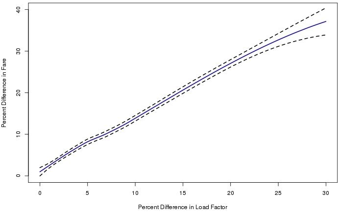
Figure 3: The role of capacity in explaining fare variation
Nonparametric regression of difference in fare by difference in load factor from
comparing fares and load factors for one-way itineraries where two flights are
available. n = 20, 062.
Figure 3 shows nonparametric fitted values as well as the 95% confidence interval of these
calculations in percentage terms. The plot suggests that when the two options have the same
number of seats occupied, the average difference in fare is close to zero. If one option is 20% more
full, the flight which is more full is also 25%, or roughly $60, more expensive. The line remains
upward sloping throughout observed differences in load factor, where at the extreme, a flight that
is 30% more full is also 35% more expensive.18
18
Applying similar methodology to round trip itineraries with two options – a single outbound flight and the choice
of two return flights, or two outbound flights and a single return flight – yields similar results.
14I perform a similar analysis using the entire sample by calculating the mean difference in fare
and load factor at the flight number, day before departure level. Figure 4 shows nonparametric
fitted values of this procedure. The line is again upward sloping across differences in load factor,
where flights with lower load factor compared to the average are also less expensive. Likewise,
flights that that have a higher occupancy compared to the average are also more expensive.
Figure 4: Lowess of mean differences in fare and load factor.
2.4.3 Do consumers dynamically substitute across booking days?
The booking curve of flights plotted in Figure 13 is smooth, even though fares tend to increase by
nearly $50 when crossing the advance purchase discount thresholds. This result is surprising since
bunching in sales should be seen before the discounts expire if consumers anticipate systematic fare
hikes. This is not the case as the only noticeable jump in load factor appears right before flights
leave. I test for discontinuities in the booking curve using regressions of the following form:
−−−→
LF = APD + m(t) + u + ε,
−−−→
where APD are dummy variables corresponding to the day before advance purchase discounts
expire, m(t) is a flexible function in time, and u are other fixed effects. Regression results appear
in Table 6. Across all specifications, I find that none of the advance purchase discount dummies are
significant; moreover, the 21 and 3 day advance purchase discount dummies are negative, which is
inconsistent with bunching.
15The fact that the there is no evidence of bunching suggests that consumers either do not
anticipate the fences or are possibly restricted in some other way from being able to purchase before
the advance purchase discounts expire. Alternatively, it could be the case that consumers substitute
to a different departure date, however this does not explain why the booking rate is similar after
the discounts expire. I use this feature of the data to motivate a demand system where consumers
do not dynamically substitute across booking days. Further, I show after estimating the model
that since prices tend to increase across time, this provides little incentive for consumers to wait
to purchase tickets.
3 A Model of Dynamic Airline Pricing
In this section, I write down a structural model of dynamic airline pricing where firms face a
stochastic arrival of consumers, and the mix of consumer types – corresponding to leisure and
business consumers – is allowed to change over time. To make the analysis tractable, I incorporate
the following simplifications in the model. First, the model studies the pricing decisions of airlines
operating in monopoly markets. In this way, the paper can focus on intertemporal price discrim-
ination and stochastic demand, and avoid the complexities of modeling oligopolistic competition.
As noted earlier, a large fraction of airline routes are monopoly. Second, I assume that when con-
sumers first learn about their interest in travel, all travel plan uncertainty is immediately resolved.
Consumers pay a fixed cost to come back and check on fares. Since fares tend to increase over time,
the combined effect of these assumptions reduce the consumer problem to a static choice of either
purchasing a ticket the day the consumer’s travel plans are realized, or not buying at all. Third,
while in the actual airline business two consumers buying on the same day might face different
fares (e.g. from different fare categories, or buying at different times of the day, or from different
web sites), in the model a single fare is offered to consumers each day. Fourth, I model consumers
as purchasing one-way tickets. A consumer interested in a round-trip can be thought of as two
consumers interested in one-way tickets. As noted earlier, in the collected data, round-trip fares
are very close to the corresponding one-way fares. Fifth, I assume firms utilize a finite set of fares.
Firms take the set as given, and choose a single fare to offer for each flight daily. This assumption
captures the fact that only a discrete number of fares is seen in the data. Finally, I assume firms do
not oversell flights since most of the routes studied are operated by an airline that does not oversell
flights. If demand exceeds remaining capacity, tickets are rationed.
163.1 Consumer Problem
A market is defined as an origin, destination, search date, departure date. At time t, M̃t ∈ N
consumers arrive interested in traveling between the two cities.19 For each of these newly-arrived
consumers, all uncertainty about travel preferences is resolved at this point. This assumption
differs from Lazarev (2013) and earlier theoretical work, including Gale and Holmes (1993), where
consumer uncertainty exists and this uncertainty can be resolved by delaying purchase until closer to
the departure date. In my model, when the date t consumers arrive, they choose to either purchase
a ticket on an available flight, exit the market, or pay a cost φ to search again the following day.
Throughout the rest of this section and when estimating the model, I assume φ is sufficiently large
so that waiting is never optimal. In Section 5.3, I calculate a bound on φ for this assumption to
hold, and show that it is relatively small – since fares tend to increase, there is little incentive to
wait.
Preferences of consumers follow the earlier two-type consumer approach to study airline markets
(Berry, Carnall, and Spiller (1996) and Berry and Jia (2010)). Consumer i is either a business
traveler or a leisure traveler. With probability γt , consumer i is a business traveler. Consumer i
receives indirect utility from product characteristics Xjt ∈ RK and price pjt . Let βi , αi denote the
taste parameters over Xjt and pjt , respectively. Let 0 denote the outside option. Each consumer i
receives idiosyncratic shocks εijt for each of the flights offered. Let εi0t be the taste shock for the
outside option. Following the discrete choice literature, consumer i chooses flight j iff
Uijt (X, p, β, α, ε) ≥ Uij 0 t (X, p, β, α, ε), ∀j 0 ∈ J ∪ {0}.
I assume utility is linear in product characteristics and of the form
Uijt = Xjt βi − αi pjt + ijt .
Let εi = (ε0i , ε1i , ..., εJi ) be the idiosyncratic preference shocks for products in the choice set
for consumer i. Define yt = αi , βi , εi i∈1,..,M̃t to be the vector of preferences for the consumers
that enter the market. The demand for flight j at t is a mapping given fares (pt ) and consumer
preferences (yt ), defined as
M̃t h
X i
Qjt (p, y) := 1 Uijt (X, p, β, α, ε) ≥ Uij 0 t (X, p, β, α, ε), ∀j 0 ∈ J ∪ {0} 7−→ {0, ..., M̃t },
i=0
19
More broadly, since M̃t is market specific, M̃t,d consumers look to travel on d, M̃t,d0 consumers look to travel on
date d0 , etc.
17where 1(·) denotes the indicator function.20
Let st ∈ NJ denote the remaining capacity for the J flights at time t, and let sjt define the
capacity for a particular flight. Demand is integer-valued; however, it may be the case that more
consumers want to travel than there are seats remaining, i.e. Qjt (p, y) > sjt . Since firms are
not allowed to oversell, in these instances, I assume remaining capacity is rationed by random
selection. Specifically, I assume the market first allows consumers to enter and choose the product
that maximizes utility. Consumers have no knowledge of remaining capacity so the probability of
not getting a seat does not affect purchasing decisions. After consumers choose the flights that
maximize their utility, the capacity constraints are checked. If demand exceeds capacity for a
particular flight j, consumers that selected flight j are randomly shuffled. The first sjt are selected
and the rest receive their outside option.
Recall that a market is departure date-specific. Although the model assumes consumers arrive
and purchase a single one-way ticket, the model does allow for round-trip ticket purchases in the
following way. At time t, two consumers arrive. One consumer is interested in leaving on date d,
and another consumer is interested in returning on date d0 . The consumers receive idiosyncratic
preference shocks for each of the available flights, and choose which tickets to purchase. Since the
round-trip fares in the sample are very close to the sum of the corresponding one-ways, there is
little measurement error in this approach.
3.2 Monopoly Pricing Problem
A monopolist sells tickets for J flights over a finite horizon. Period T corresponds to the first
period of sale, and t = 0 is the time at which the flights depart. Each flight has an initial capacity
constraint of sjT seats, which is exogenous to the model. I assume the cost of operation is sunk, so
the only cost facing the firm is the opportunity cost of selling seats.21
The firm maximizes expected discounted revenues. The firm knows on average how many
business and leisure travelers will search for tickets over time, but is unsure exactly how many
consumers will arrive in any given period. Since fares are posted before consumers arrive, the firm
forms expectation over present and future revenues. The decision rule depends on the number of
seats remaining and the number of periods left to sell. 22
20
Here, and for remainder of the paper, I suppress the dependence of Q on X to emphasize the role of price. X
may contain a flight characteristics such as whether a particular flight is a morning or afternoon flight. In addition,
X may contain an indicator for a particular departure date which would allow the firm to use peak-load pricing.
21
I assume the marginal cost per passenger is zero, which is reasonable as almost all flight costs are not influenced
by the number of seats occupied.
22
The decision may also depend on other observed (at least to the firm) states Zt . Note that X ⊂ Z since all
product characteristics that enter the consumer problem affect purchasing behavior, and consequently, affect expected
revenues. Like X, I suppress the notation of Zt to highlight the importance of remaining capacity st in the firm
problem.
18Since excess demand is rationed, by charging prices pt and receiving consumers yt , the firm can
sell at most min(Qt (p, y), st ) seats, where min(·) is element-wise. This implies the law of motion
for remaining capacity can be written as
st−1 = st − min Qt (p, y), st .
Define the incremental revenue for the firm to be
Rt (p, y, s) = min Qt (p, y), st · pt .
The firm is restricted to choosing prices pt ∈ P(st ), where the dependence on seats is noted since
only flights with positive remaining capacity are priced.
To write the firm’s problem as a dynamic program, define the value function, Vt (s) to be the
discounted expected revenue left to go with remaining capacities st and t periods to sell. The
restrictions on capacity form two boundary conditions on the value function. The first is that with
zero seats remaining, the firm cannot capture additional revenue, which is Vjt (0) = 0. Second,
unsold seats the day the flights leave must be scrapped with zero value implying Vj0 (s) = 0.
The firm’s problem can be written recursively as
h i
0
Vt (s) = max Ey Rt (p, y, s) + ρVt−1 (s | y, s)
pt ∈P(st )
st−1 = st − min Qt (p, y), st
Vj0 (s) = 0
s.t.
Vjt (0) = 0
st given,
where ρ ∈ [0, 1] is the discount factor (which I set equal to 1).
The value function of the firm illustrates the important interactions between intertemporal price
discrimination and dynamic adjustment to stochastic demand. If business consumers are less price
sensitive and the proportion of business consumers increases as the departure date approaches, the
firm can extract more revenue by increasing fares over time. However, since the arrival of consumers
is uncertain, it is possible that a flight may sell out early. This creates an incentive for the firm
to save seats until close to the departure date. Looking at the value function, if capacity becomes
scarce early on, the firm can increase fares to reduce current period expected sales and revenues,
but increase the probability that seats will remain the following day. For example, if the firm sets
19pt = ∞, then current period expected revenues would be zero, but the probability that st = st−1
would be one. Hence, the firm would enter the subsequent period under Vt−1 (st ) which may be the
optimal pricing strategy if the firm expects high-valuing consumers to arrive closer to the departure
date. Alternatively, it may be the case that the firm receives a sequence of low demand realizations.
In order to not leave as many seats unfilled, the firm may opt to lower prices.
3.3 Offering a single flight
Most markets in my sample have one flight a day. I concentrate my analysis to these flights as it
greatly simplifies the demand system, as shown in Section 4. When a single flight is offered daily,
the monopolist does not need to worry about substitution across flights. Recall that the firm does
not know exactly how many consumers nor how many consumers of each type will arrive before the
pricing decision is made. This is why the firm takes expectation over yt . With just a single flight
offering, the expected sales for the flight is
Z
Qet (s, p) = min Qt (p, y), st dF (yt ).
yt
By charging a price pt , the firm has a probability distribution over remaining capacity tomorrow.
The value function for the firm can be rewritten as
h i
Vt (s) = max pt Qet (s, p) + ρE[Vt−1 (s0 |s)]
pt ∈P(st )
st
X
= max pt Qet (s, p) + ρ Pr(st−1 = j | pt , st )Vt−1 (j) .
pt ∈P(st )
j=0
such that st−1 = st − min Qt (p, y), st and the two boundary conditions hold.
The optimal pricing policy of the firm, p(t, s; θ), depends solely on the consumer demand pa-
rameters θ, including taste preferences, the mix of consumer types, and the arrival process. In the
next section, I discuss estimation of these parameters.
4 Econometric Specification & Estimation
I first parameterize the demand model and derive analytic expressions for purchase probabilities.
I model the firm’s pricing decision as a dynamic discrete choice model. To estimate the structural
parameters of the model, I solve the dynamic program of the firm.
204.1 Consumer Demand
First I derive the purchase probabilities for the consumer demand system. Recall that the prefer-
ences of consumers that arrive to the market are
yt = αi , βi , εi i∈1,..,M̃t
.
The number of consumers, as well as the relative proportion of each type, that will arrive is not
observed by the firm before pricing (or by the econometrician). In order to proceed, I integrate
over the distribution of yt .23
Assumption 1: Consumer idiosyncratic preferences are distributed Type-1 Extreme Value (T1EV).
I assume the outside option yields a normalized utility ui0t = εi0t . The distributional assumption
on the idiosyncratic preferences leads to the frequently used conditional logit demand system. Since
there is only a single product in the choice set,
1
ςti := Pr(i wants to purchase j|type = i) = .
1 + exp(−Xjt βi + αi pjt )
The discrete choice literature typically does not model capacity constraints. Given my environment,
it is possible that consumers wish to purchase a product, but are unable to due to a violation of the
capacity constraint. As noted in the previous section, if demand exceeds available capacity, demand
is rationed, and consumers who are not selected for travel receive their outside option. This is why
i denote
the purchase probabilities state “i wants to purchase j” instead of “i purchases j”. Let ς0t
the share of the outside option.
In practice, appropriate data to enter X would be variables such as if a flight is operated on a
holiday or weekend. Preferences over these characteristics could also vary across consumer types
and/or routes. While the model allows for these covariates, I assume consumers only care about
price, which is not unreasonable as the routes studied are monopoly with a single flight daily.24
Let B denote the business type and L to denote the leisure type. The probability of a consumer
being type-B is γt . Then γt sB
t defines the probability that a consumer is of the business type and
wants to purchase a ticket. Consider the market share of the outside good at time t. Conditional
on k consumers arriving, the probability of zero consumers wishing to travel is
k
X k L
i
B
k−i
Pr Qt = 0 | k ∈ N = (1 − γt )ςt0 γt ςt0 .
i
i=0
23
I proceed this way because individual decisions are not observed. Using the EM-algorithm would be another way
to address this issue. See: Talluri and Van Ryzin (2004) and Vulcano, van Ryzin, and Chaar (2010).
24
When I solve the firm problem, adding additional characteristics makes the problem very computationally de-
manding. I do allow all parameters to be route-specific.
21For example, let k = 2. Then conditional on two consumers arriving, both consumers want to
purchase the outside option. Either both consumers are leisure travelers, both consumers are
business travelers, or one of each type arrive. The first two situations correspond to i = 2 and
L )2 is the probability of two leisure consumers arriving and
i = 0, respectively since ((1 − γ)ςt0
B )2 is the probability two business consumers want to
wanting to choose the outside option, and (γςt0
choose the outside option. Lastly, it could be the case that one business and one leisure consumer
arrives. There are two possibilities, the first consumer is the business consumer, or vice versa.
Hence, 2[(1 − γ)ς0L ][γς0B ] enters the probability.
Next, integrating over the arrival process of consumers yields
X∞ ∞
X
Pr Qt = 0 = Pr(Qt = 0, M̃t = k) = Pr(Qt = 0|M̃t = k)Pr(M̃t = k).
k=0 k=0
Assumption 2: Consumers arrive according to a Poisson process, M̃t ∼ Poisson(µt ).25
The probability mass function for the Poisson distribution is (µt )k e−µt /k!, k ∈ N. With this
assumption, Pr Qt = 0 has an analytic form and can be written as
∞ k
X µkt e−µt X k L
i
B
k−i
Pr Qt = 0 = (1 − γt )ςt0 γt ςt0 .
k! i
k=0 i=0
Implicitly, this depends on both price and capacity remaining. With zero seats remaining, price is
L = ς B = 1, which implies Pr Q = 0 = 1, as expected. Next, consider the probability
infinite so ςt0 t0 t
of selling a positive number of seats, but not selling out, conditional on k. This probability can be
written as
k X q
q ` q−`
Pr Qt = q | k ≥ q, q < s = γt ςtB (1 − γt )ςtL ×
q `
`=0
"k−q #
X k − q i k−q−i
L B
(1 − γt )ςt0 γt ςt0 .
i
i=0
In the formula above, the terms following the first sum correspond to all the combinations of having
q consumers wanting to purchase a ticket. The terms following the second summation (second line)
correspond to all the combinations of the remaining k − q consumers wanting to purchase the
outside option. Finally, kCq at the beginning of the equation sorts all the possible combinations of
(want to buy, do not want to buy) amongst the q of k consumers that wish to purchase tickets. Of
25
Given this assumption, the demand model closely follows Talluri and Van Ryzin (2004) and Vulcano, van Ryzin,
and Chaar (2010), except this model has two consumer types.
22course, selling q seats requires at least k = q consumers to enter so Pr(sell q | k < q, q < C, p) = 0.
Integrating over the Poisson arrival process results in an analytic expression for Pr(sell q | q < C, p),
which is also a Poisson-Binomial mixture.
Demand is latent in situations where flights are observed to sell out since it is possible some
consumers are forced to the outside option. These probabilities can be constructed based off the
fact that at least st seats are demanded. For example, if st = 2 and the flight is observed to
sell out, that implies at least 2 seats were demanded, which also has an analytic expression of a
Poisson-Binomial mixture. Since capacity is assumed to be monotonically decreasing, all purchase
probabilities have been defined, which appear in Equation 4.1 - Equation 4.3 below. Collectively
call these probabilities f (s0 |s, p, t).26
∞ X ∞ q
X µkt e−µt k X q B ` L
q−`
Pr Qt ≥ s | s, p = γt st (1 − γt )st × (4.1)
q=s k=q
k! q `
`=0
"k−q #
X k − q i k−q−i
(1 − γt )st 0L γt sB
t0
i
i=0
∞ q
X µkt e−µt k X q B ` q−`
Pr Qt = q | 0 < q < s, p = γt s t (1 − γt )sL t × (4.2)
k! q `
k=q `=0
"k−q #
X k − q i k−q−i
L B
(1 − γt )st0 γt st0
i
i=0
∞ k
X µkt e−µt X k i k−i
Pr Qt = 0 | s > 0, p = (1 − γt )sL
t0 γ s B
t t0 . (4.3)
k! i
k=0 i=0
4.2 Solving the dynamic program of the firm
The firm’s pricing decision depends on remaining capacity and time to sell. I assume fares are
chosen from a discrete set, which is exogenous to the model. I define this set to be the set of
observed fares in the data. This assumption accurately reflects that fares for any given flight tend
to fluctuate between relatively few distinct prices. This assumption allows me to write down the
firm’s problem a dynamic choice choice model.
Since the firm’s decision depends on observed states, the model cannot capture why two flights
that have the same number of seats remaining and time left to sell are priced differently in the
data. To account for this, I assume the firm faces states (ω(pt ))pt ∈P(st ) , which are choice-specific
26
To be clear, s0 denotes the number of seats sold in the current period given remaining capacity s.
23You can also read