Climate resilient interconnected infrastructure: Co-optimization of energy systems and urban morphology
←
→
Page content transcription
If your browser does not render page correctly, please read the page content below
Climate resilient interconnected infrastructure: Co-optimization
of energy systems and urban morphology

Downloaded from: https://research.chalmers.se, 2021-07-15 16:13 UTC

     Citation for the original published paper (version of record):
     Perera, A., Javanroodi, K., Nik, V. (2021)
     Climate resilient interconnected infrastructure: Co-optimization of energy systems and urban
     morphology
     Applied Energy, 285
     http://dx.doi.org/10.1016/j.apenergy.2020.116430

N.B. When citing this work, cite the original published paper.

research.chalmers.se offers the possibility of retrieving research publications produced at Chalmers University of Technology.
It covers all kind of research output: articles, dissertations, conference papers, reports etc. since 2004.
research.chalmers.se is administrated and maintained by Chalmers Library

                                           (article starts on next page)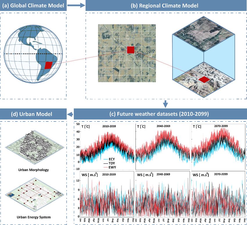
Applied Energy 285 (2021) 116430
Contents lists available at ScienceDirect
Applied Energy
journal homepage: www.elsevier.com/locate/apenergy
Climate resilient interconnected infrastructure: Co-optimization of energy
systems and urban morphology
A.T.D. Perera a, *, 1, Kavan Javanroodi b, c, 1, Vahid M. Nik c, d, e
a
Urban Energy Systems Laboratory, EMPA, Überland Str. 129, 8600 Dübendorf, Switzerland
b
Solar Energy and Building Physics Laboratory (LESO-PB), Ecole Polytechnique Fédérale de Lausanne (EPFL), CH-1015 Lausanne, Switzerland
c
Division of Building Technology, Department of Architecture and Civil Engineering, Chalmers University of Technology, SE-41296 Gothenburg, Sweden
d
Division of Building Physics, Department of Building and Environmental Technology, Lund University, SE-22363 Lund, Sweden
e
Institute for Future Environments, Queensland University of Technology, Garden Point Campus, 2 George Street, Brisbane, QLD 4000, Australia
H I G H L I G H T S
• Novel optimization algorithm to optimize both urban morphology and energy system.
• Building form and urban density will increase in the energy demand by 10% and 27%.
• The influence of urban morphology on energy system cost can be up to 50%.
• Co-optimization of both urban morphology and energy system is vital maintain climate resilience.
A R T I C L E I N F O A B S T R A C T
Keywords: Co-optimization of urban morphology and distributed energy systems is key to curb energy consumption and
Interconnected infrastructure optimally exploit renewable energy in cities. Currently available optimization techniques focus on either
Energy systems buildings or energy systems, mostly neglecting the impact of their interactions, which limits the renewable
Urban form
energy integration and robustness of the energy infrastructure; particularly in extreme weather conditions. To
Urban planning
Sustainable cities
move beyond the current state-of-the-art, this study proposes a novel methodology to optimize urban energy
systems as interconnected urban infrastructures affected by urban morphology. A set of urban morphologies
representing twenty distinct neighborhoods is generated based on fifteen influencing parameters. The energy
performance of each urban morphology is assessed and optimized for typical and extreme warm and cold
weather datasets in three time periods from 2010 to 2039, 2040 to 2069, and 2070 to 2099 for Athens, Greece.
Pareto optimization is conducted to generate an optimal energy system and urban morphology. The results show
that a thus optimized urban morphology can reduce the levelized cost for energy infrastructure by up to 30%.
The study reveals further that the current building form and urban density of the modelled neighborhoods will
lead to an increase in the energy demand by 10% and 27% respectively. Furthermore, extreme climate conditions
will increase energy demand by 20%, which will lead to an increment in the levelized cost of energy infra
structure by 40%. Finally, it is shown that co-optimization of both urban morphology and energy system will
guarantee climate resilience of urban energy systems with a minimum investment.
1. Introduction 2030) [2]. This massive urban development has significantly changed
the morphology of cities, as new multi-functional urban areas appear
Due to rapid urbanization [1], cities are witnessing a drastic growth. within and beyond the borderline of megacities. Cities and urban areas
The number of cities with a population of five hundred thousand to one are characterized by their high energy density and heterogeneity in
million is currently estimated to increase from 598 (in 2016) to 710 (in energy use profiles [3]. They accommodate around 50% of the world’s
* Corresponding author.
E-mail addresses: dasun.perera@empa.ch (A.T.D. Perera), kavan.javanroodi@epfl.ch (K. Javanroodi).
1
These authors contribute equally.
https://doi.org/10.1016/j.apenergy.2020.116430
Received 28 August 2020; Received in revised form 5 December 2020; Accepted 30 December 2020
Available online 10 January 2021
0306-2619/© 2021 The Author(s). Published by Elsevier Ltd. This is an open access article under the CC BY license (http://creativecommons.org/licenses/by/4.0/).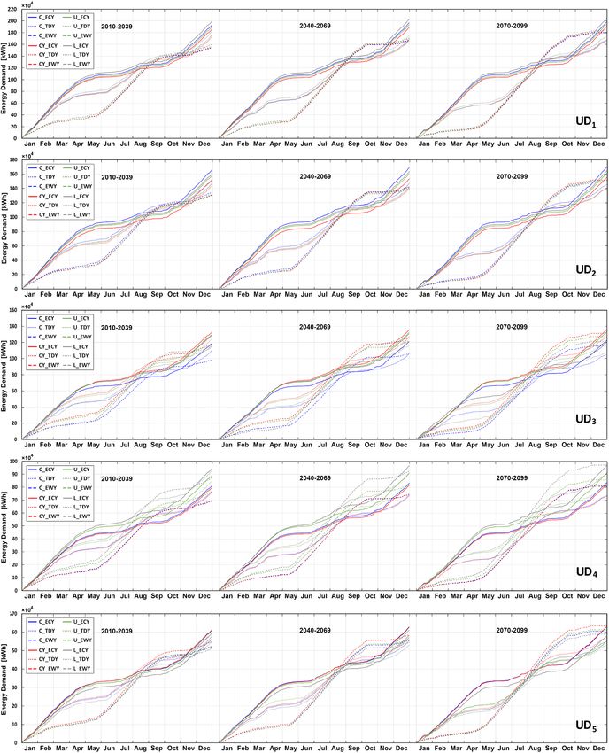
A.T.D. Perera et al. Applied Energy 285 (2021) 116430
population [4] and are responsible for two-thirds of the global primary Climate change complicates the design problem due to its multi-
energy consumption, inducing 71% of global direct energy-related dimensional impacts on both the energy and the building sector as
greenhouse gas (GHG) emissions [5,6]. It is projected that due to pop well as due to the considerable uncertainties that exist in climate change
ulation growth in urban areas, 68% of the world’s population will live in projections [31]. The sequential method applied in the present state of
urban areas by 2050 [4]. This, together with climate change and eco the art, in which urban planning is performed as a sequential process
nomic growth will place enormous pressure on material and energy where decisions related to urban morphology are taken first and fol
resources [7]. lowed by energy system designis unsuitable to deal with this level of
It is widely known that energy demand in urban areas is highly complexity [32,33]. The thermal performance of urban morphologies
affected by climate variations [8]]. Increasing the share of renewable can significantly change due to extreme climate events such as heat
energy generation based on distributed energy sources, such as solar and waves, ultimately collapsing the energy infrastructure [9,10]. This
wind energy, will increase the dependence of energy supply on climate highlights the importance of harmonizing the urban planning and the
and can change the roles and relations in the energy market [9]. Climate energy system optimization process, which demands a major change in
change including extreme events can considerably influence the reli methods used for energy system design and urban planning.
ability and resilience of energy systems, affecting different aspects of the Reaching a higher level of energy sustainability and climate resil
energy flow from generation to demand [10]. Reaching a win-win sit ience in cities requires developing frameworks that concurrently opti
uation where both climate change mitigation and adaptation are ful mize the urban morphology and the energy system while accounting for
filled requires understanding the interactions between variations in their interconnected interactions. This study develops such a frame
climate, energy demand and supply. It is vital to consider the climate work, considering the following objectives:
dependence of the energy demand and supply and to accommodate their
variations in the energy system design when planning to increase the • Developing a co-optimization algorithm that can facilitate layout
sustainability and resilience of energy systems [11]. The energy condi planning for the building sector as well as optimize energy system
tions are also strongly influenced by the sectoral and technical changes design. Understanding the connectivity between building and energy
that take place in cities and urban areas, such as increased urbanization infrastructure plays a vital role in this regard which has not been
and electrification of transport [8]. This means that the energy system is discussed in the present state of the art. Optimizing both building
an interconnected urban infrastructure with complex interactions with and energy infrastructure considering
climate, urban morphology, urbanization, etc. 1. Urban form
Urban morphology has a considerable impact both on the energy 2. Urban density
sustainability and the climate resilience of cities. In the process of ur 3. Energy system design (capacity of energy system components)
banization, the main elements of urban morphology, such as urban form 4. Operation strategy implemented by the energy system
(e.g. density, shape, layout, height, etc.), urban function (e.g. functional
needs of buildings, size, location, etc.) and urban pattern (e.g. streets, is performed in this study.
canopies, open spaces) have transformed into far more complex inter
connected urban structures [12,13]. The complexity of urban • Evaluate the impact of future variations on energy optimized design
morphology is one of the major drivers of climate variations at urban to assess climate resilience, since future climate variations and
and local scale [14]. Urban climate can be defined as the interactions extreme climate events can have a notable impact on the energy
between urban morphology elements and climate variables [15]. More demand as well as on renewable energy generation, especially
specifically, air temperature, wind flow patterns [16], relative humidity considering extreme conditions.
[17], and solar radiation [18] are considerably affected by morpholog
ical elements. Among other, urban morphology can modify the amount In this work, the focus is mainly on the interactions between the
of shading [19] and desirable/undesirable solar radiation in urban areas energy system (demand, supply and system design), outdoor climate and
[20]. This can increase the dependence of buildings on air conditioning urban morphologies. The scope of the study is limited to these three
systems to maintain thermal comfort [21] as well as the electricity major interacting factors, aiming to avoid increasing uncertainties in the
required to provide desired lighting [22]. A clear link also exists be assessment, understand the interactions, investigate the probable cor
tween urban morphology and renewable energy potential in urban areas relations and reach viable results. The research paper is organized as
[23,24], which demonstrates the importance of urban morphology from follows: Section 2 of the manuscript presents the workflow that links the
the perspectives of energy efficiency and sustainability. future climate model with the urban simulation model and the energy
A number of recent studies have focused on improving the efficiency system model. Section 3 presents the model used to generate climate
of urban forms. Natanian et al [25], proposed a framework to optimize files required for the building and energy system design process with the
generic urban forms in terms of energy demand and spatial daylight support of regional and global climate models. Section 4 presents an
autonomy. Ye et al [26], assessed different methods to optimize urban overview of the computational model used for the urban simulation,
forms to reduce CO2 emissions. Martins et al [27], introduced a multi- which generates the energy demand profiles for a set of different urban
objective optimization framework to optimize solar energy potential morphologies. The co-optimization of urban form and the energy system
in a simplified urban form. Only a few studies focus on the impacts of are explained in the latter part of Section 5. Finally, Section 6 is devoted
urban morphology on urban energy system design and renewable en to discussing the results of the study followed by conclusions to pre-sent
ergy integration [28]. Perera et al. [29,30] showed that urban density as the major findings of the study in Section 7.
well as building layout have a notable impact on investment and oper
ation cost, renewable energy integration and autonomy level of urban 2. The workflow of the computational model
energy systems. According to their studies, certain building layouts will
facilitate higher integration levels of renewable energy technologies Urban energy planning is too complex to be handled by a single
while minimizing the cost (of both operation and investment) of the computational model. Therefore, computational platforms that link
energy systems. However, it is impossible to define an optimal urban several models are often developed to achieve this task. For example,
layout that can be used universally since it depends on the local seasonal Guan et al. [34] and Mohajeri et al. [28] developed a computational
changes in climate, energy demand patterns as well as renewable energy platform linking a GIS module, an urban simulation module and an
generation potential. Instead, it makes sense to develop methodologies energy system design module to support energy planning for a Swiss
to optimize urban morphology considering energy as well as climate village. A similar workflow is not necessarily adequate to assess the
resilience. impacts of climate change. To do so, the workflow needs to be able to
2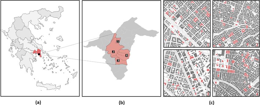
A.T.D. Perera et al.                                                                                                               Applied Energy 285 (2021) 116430

Fig. 1. Workflow of the study in five major steps including generating urban morphologies (Step 1), and future weather datasets (Step 2), energy simulations (Step
3), assessing renewable energy potential (Step 4), collecting techno-economic data (Step5), and achieving optimal system design and urban morphology (Step 6).

              Fig. 2. Moving from global climate models to weather data at the urban scale to be used in design optimization of urban energy systems.

                                                                                 3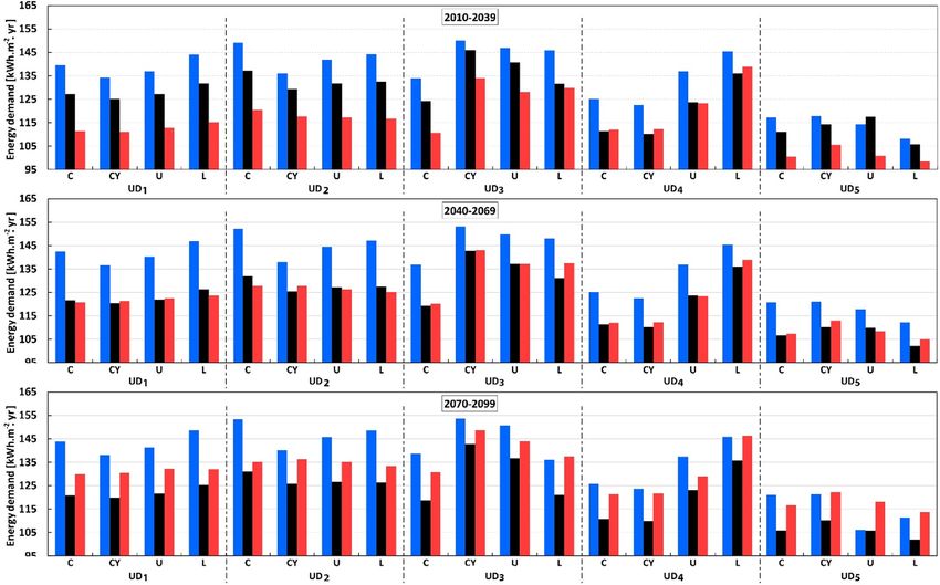
A.T.D. Perera et al. Applied Energy 285 (2021) 116430
handle large weather data sets and climate uncertainties or to generate consistent weather data across different variables with the temporal and
representative weather data sets from climate models [35]. Moreover, it spatial resolutions suitable for energy simulations [39]. The spatial
should be able to take into account climate variations with fine temporal resolution of RCMs is mostly between 10 and 50 km (mesoscale),
and spatial resolutions (e.g. hourly variations minimum at the mesoscale although there exist a few with finer resolutions, even down to 2.5 km.
and preferably at the urban-scale) and their impacts on both energy However, RCMs mostly do not consider the impacts of urban texture and
demand and supply. These all mean that the workflow should be able to energy flows in the urban scale since this usually needs downscaling to
provide a seamless transfer of weather data from climate models to spatial resolutions of less than 1 km. Meanwhile, at the urban- and
energy models, either its own or representative weather data sets that micro-climate scale, considerable variations may occur to mesoscale
take into account climate uncertainties as well as both typical and weather, amplifying or dampening extreme weather [14] and influ
extreme conditions [31]. Therefore, the workflow of the urban planning encing the energy performance of buildings [9].
process is extended in this study to include the inputs from climate In this work, the microclimate around buildings has been simulated
models as presented in [10] and shown in Fig. 1. using the weather data simulated by RCA4 [40], which is the 4th gen
The workflow presented in this work, first generates representative eration of the Rossby Centre RCM. When doing an impact assessment of
future weather files as presented in Section 3 and uses them in urban climate change, it is not considered appropriate to rely on only a few
climate modelling and energy simulations. The workflow begins with climate scenarios and short term periods [39]. Multiple climate sce
formulating urban archetypes as described in Step 1, urban simulation is narios (e.g. with different GCMs and RCPs) should be considered for
performed to identify the energy demands in the future considering study periods of 20–30 years, which increases the computational load
typical and extreme weather conditions. Step 2 presents climate data for extensively [31]. Nik [31] developed a method to overcome the chal
the urban simulation conducted in Step 3. Future climate weather data is lenges of big data sets and climate uncertainties. The method is based on
used to obtain renewable energy generation potentials as presented in synthesizing three sets of representative future weather data sets out of
Step 4. Technoeconomic data is collected in Step 5, and finally used to RCMs: Typical Downscaled Year (TDY), Extreme Cold Year (ECY), and
arrive at an optimal system design and urban morphology in Step 6. The Extreme Warm Year (EWY). The three synthesized one-year-long
representative weather data sets, including typical and extreme weather weather data sets represent typical and extreme weather conditions
conditions, are used in the urban simulation model to generate energy while considering multiple climate scenarios. This has the advantages of
demand for heating, cooling and electricity for different alternative shortening the analysis time considerably while still accounting for
urban morphologies. The urban energy simulation model considers the climate uncertainties and extremes. The application of the method has
weather conditions, interactions among buildings (shading effect), oc been compared with other available approaches and weather data sets
cupancy in buildings, lighting conditions and equipment usage at the [41] and verified for several types of simulations and impact assess
building level when computing the energy demand for each ments [31]. The method has been developed further to quantify the
morphology. A comprehensive explanation of the urban simulation impacts of climate change on urban energy systems [10]. In this work,
model is presented in Section 4. two groups of data sets have been generated; one for calculating the
Subsequently, a pool of time-series corresponding to different urban energy demand based on the method in [31] and one for renewable
morphologies are used to find the optimal urban morphology. The generation potentials based on the method in [10]. Representative
generated time-series of energy demand for the considered urban mor weather data sets have been synthesized for the three 30-year periods of
phologies are used to optimize the urban morphology (form and density) 2010–2039, 2040–2069, and 2070–2099, considering 13 future climate
along with the energy systems. The energy system optimization model is scenarios (five different GCMs and three RCPs: RCP 2.6, RCP 4.5 and
used to size the energy system, i.e. to define the optimal capacities for RCP 8.5). For more details about synthesizing the weather files, the
dispatchable energy sources, non-dispatchable renewable energy tech reader is referred to [31,10].
nologies such as wind and solar PV, energy storage, and energy con As mentioned above, RCM outputs, which are meso-climate, can be
version devices such as heat pumps. Usually, this is formulated as a bi- considered as weather data, reflecting the conditions and variations that
level optimization problem considering dispatch optimization at the affect energy performance of buildings, energy systems and human
primary level and the system configuration optimization at the sec comfort (Fig. 2). Using mesoscale climate data (with the horizontal
ondary level. Energy demand is considered as an input parameter to the resolution of 5–100 km) for energy simulations is widely practiced and
energy design model, which does not depend on the decision vector. The accepted by the scientific community. Although buildings and in
main change introduced in this study is that we consider urban form and frastructures are affected by the urban/micro-climate around them, it is
urban density as a decision vectors. As a result, energy demand is subject very rare to use such high-resolution climate for energy simulations due
to vary with the decision vector, which enables a concurrent definition to lack of access to observed/simulated weather data and their strong
of optimal design and urban form. A comprehensive explanation of the case dependency (i.e. valid for the specific cases that the urban/micro-
formulation of objective functions is presented in Section 5. climate have been observed or simulated). Therefore, so far the com
mon approach in the energy simulation community has been using
3. Climate models and developing extreme climate conditions meso-climate data. For example, all the available and ready to use
weather data sets for energy simulation tools (like the well-known TMY
Global climate models (GCMs) are used to simulate future climate. format) are meso-climate [42]. As is reviewed and discussed thoroughly
GCMs are forced by different concentrations of anthropogenic Green in previous works of the authors [31,41], there are different approaches
house Gas (GHG), depending on the selected Representative Concen to generate weather data sets from RCMs to be used energy simulations.
tration Pathways (RCPs), four of which are defined based on the IPCC Being able to properly count for sub-meso features and variations that
Fifth Assessment Report (AR5): RCP 2.6, RCP 4.5, RCP 6.5 and RCP 8.5, occur to weather due to the urban texture will increase the accuracy of
labeled after a possible range of radiative forcing values in the year 2100 energy simulations and better reflect the impact of extreme weather
(2.6, 4.5, 6, and 8.5 W/m2, respectively) [36,37]. GCMs have a coarse conditions, as is discussed in our previous works [14,43]. Since the most
spatial resolution of 100–300 km and their outputs cannot be considered extreme scenarios have been used in the energy simulations and analysis
weather data [38], which is required for energy simulations (check (extremes considering outdoor temperature, solar radiation and wind
Fig. 2). Therefore, GCMs are downscaled using two main approaches; speed with monthly and hourly temporal resolutions for energy demand
dynamical and statistical downscaling [31]. The statistical version only and generation calculations) considering 13 future climate scenarios
reflects changes in the average weather conditions and underestimates (390 single years) with five different GCMs and three RCPs (which RCP
extremes. Therefore, dynamical downscaling (using regional climate 8.5 is considered as the worst case scenario), we can be very confident
models or RCMs) is recommended, which simulates physically that the most pessimistic and extreme scenarios are considered in the
4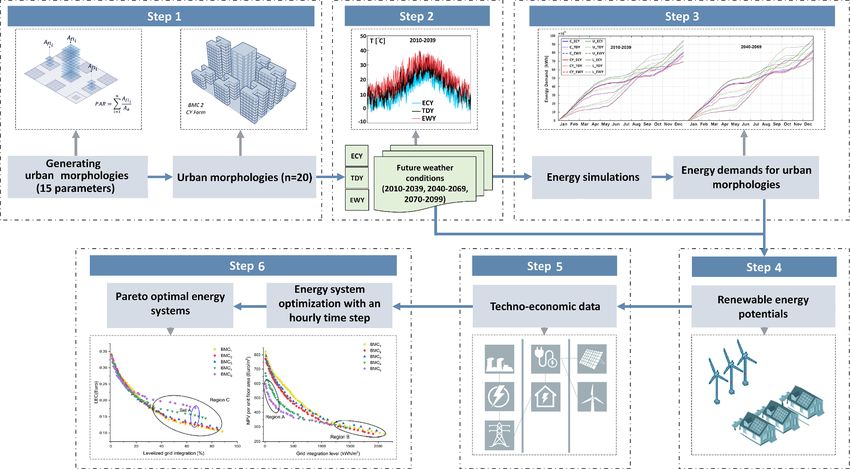
A.T.D. Perera et al. Applied Energy 285 (2021) 116430
Fig. 3. (a) Athens, Greece, (b) Central Athens, the studied area in this paper, (c) site plan of four urban areas with different physical characteristics.
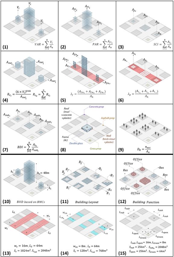
resilience assessment. density index (BDI), urban plan area density (λp), frontal area density
(λf), relative compactness (Rc), building materials, and occupancy
4. Case study and urban morphologies density (Doc), and Urban Form (including building layout and building
height distribution or ‘BHD’, neighborhood size, building function,
Representing urban complexity through a set of alternative mor streets and canopies geometry and materials) based on their morpho
phologies requires selected morphologies to be matched with the local logical definitions. Table A1 in Appendix presents a description of each
conditions while presenting energy-efficient alternatives. Section 4.1 parameter and Fig. 4 illustrates the graphical definition of them.
presents a brief overview of the considered case study elaborating the A hypothetical site with a total area of 5120 m2 is defined as a
local conditions while Section 4.2 describes the process used to generate template to generate an urban neighborhood (20 × 16 grid). The defined
alternative urban morphologies considered in the study. site is fragmented into a matrix with three rows and columns resulting in
nine equal sub-sites. Each sub-site is based on a 4 × 4 grid (covering 45%
4.1. Case study of the site) and a network of streets and canopies (covering 55% of the
site). One sub-site (covering 5% of the site) is selected as open space, in
Athens, the capital and largest city in Greece, is selected as the case which a total area of 64 m2 (covering 0.01% of the whole site, and 25%
study in this research work. It has an overall land area of roughly 414 of the sub-site) is considered as green space (there is scarcity of green
km2 and an urban population of approximately 3.2 million [44]. The spaces in the studied area). Two main streets (each 4 × 16 grid) and six
area selected for the purpose of this study is located in Central Athens canopies (each 2 × 4 grid) are defined between the nine equal sub-sites.
(hereafter referred to as Athens) with a total area of 87.4 km2, a popu To cover a wide range of urban areas in the selected case study, five
lation of about 1 million and a population density of 12,000 per 1 km2, ranges of urban densities are defined based on the adopted morpho
containing eight municipal districts [45]. The city has a subtropical logical parameters as follows:
Mediterranean climate with hot arid summers and fairly mild winters
[46,47]. High urban density, narrow streets and scarcity of green spaces (1) UD1: Horizontal: selecting 14 cells out of 16 (BDI = 87.5%),
contribute to the development of a strong urban heat island (UHI) index Vertical: BHD = 60 floors.
[48]. This results in a very large cooling demand during the summer (2) UD2: Horizontal: selecting 12 cells out of 16 (BDI = 75%), Ver
months with considerably high peak values [49]. To recognize the urban tical: BHD = 54 floors.
morphology of Athens, the most frequent physical characteristics of (3) UD3: Horizontal: selecting 10 cells out of 16 (BDI = 62.5%),
urban neighborhoods (e.g. layouts, built density, building height, etc.) Vertical: BHD = 48 floors.
were studied for each municipal district. The majority of buildings in (4) UD4: Horizontal: selecting 8 cells out of 16 (BDI = 50%), Vertical:
Athens are multi-story apartments with flat roof shapes, and high ther BHD = 40 floors.
mal mass (cement/concrete as the main material) [50–53]. Fig. 3 shows (5) UD5: Horizontal: selecting 6 cells out of 25 (BDI = 37.5%), Ver
the studied area and site plan of four urban areas with different physical tical: BHD = 34 floors.
characteristics.
Each cell represents one thermal zone with a total area of 16 m2 (a 4
× 4 m space). For urban form, four major architectural layouts are
4.2. Generating urban morphologies selected as the main design constraints in the developed version of the
BMC technique, including Cube (C), Courtyard (CY) and L and U forms.
A method introduced by Javanroodi et al.[54], “Building Modular As an attempt to define the vertical expansion of the developed layouts,
Cell” or “BMC”, is adopted in this work to generate urban morphologies . five ranges of building heights (number of floors) are considered based
BMC is based on the horizontal and vertical expansion of a basic module on the defined UD ranges. However, due to the comparative approach of
(4 × 4 × 4 m cube) to generate quadrilateral layouts in respect with this study, at the central sub-site, a twelve-story building with a height of
several design-based constraints (e.g. connectivity between modules at 48 m is placed in all twenty urban neighborhoods. Based on the location
least from one side, the generated configuration should be one inte of each cell at the outer sides (building’s elevation), a constant glazing
grated shape in each sub-site, the minimum number of floors for each ratio is defined: North elevation: 16%; West and East elevations: 8%; and
building is two and maximum is twelve). A total number of fifteen South elevation: 25%.
influencing morphological parameters are used to generate the urban According to this procedure, twenty distinct architectural layouts are
morphologies. The influencing parameters are categorized into two selected out of 400 generated building layouts using the BMC technique,
comprehensive groups of Urban Density (including plot to area ratio based on the most frequent building layouts observed in the studied
(PAR), volume to area ratio or (VAR), site coverage index (SCI), building
5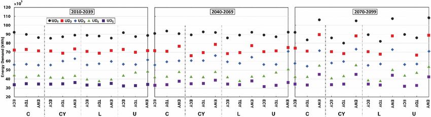
A.T.D. Perera et al. Applied Energy 285 (2021) 116430
Fig. 4. The major considered variables in this
study based on two major parameters: Urban
Density: (1) Volume Area Ratio or ‘VAR’, (2) Plot
Area Ratio or ‘PAR’, (3) Site Coverage Index or
‘SCI’, (4) Relative Compactness or ‘RC’, (5)
Frontal area density or ‘λp’, (6) Urban plan area
density or ‘λp’, (7) Building Density Index or
‘BDI’; (8) Materials; (9) Occupancy density or
‘Doc’: 0.02 and 0.035 [n/m2] for residential and
office buildings., and Urban Form: (10) Building
Height Distribution ‘BHD’, (11) Building Layouts,
(12) building function, (13) Urban pattern: main
streets, (14) Urban pattern: canopies with 120
different H/w ratios, (15) Neighborhood size.
area. Each UD category has a constant total area and number of floors cell is defined as a thermal zone with at least one connection with the
with four different architectural form (C, CY, L, U). Moreover, two adjacent cell at each architectural layout. The total number of thermal
different building types including residential and commercial (office) zones for cases in each UD category is 172, 144, 130, 109, and 88
are considered in all twenty cases as urban function parameters (with respectively for UD1 to UD5. The cooling/heating demand, equipment,
different materials, performance, heating/cooling systems, lighting/ and lighting energy demand profiles are calculated for all thermal zones
equipment, etc.). The combination of two building types will lead to a on each floor of building blocks as the combination of latent and sensible
more general and realistic representation of the energy system and the loads. The impacts of the surrounding buildings on each building are
integration of renewable energy potentials based on complex urban calculated through the true view factor algorithm in EnergyPlus, which
neighborhoods. Fig. 5 illustrates the 3D model of the urban morphol modifies the amount gained direct/diffuse solar radiation beams for
ogies generated in this study with corresponding values for each external surface of each building. The total heat transfer through
parameter. external surfaces (wall, roof, floors, and windows) as well as internal
The models generated in Grasshopper are converted and exported loads (e.g. people density, Equipment, Lightning, etc.) and infiltration
into EnergyPlus models using Archsim, Diva for Rhino 4.0 plugin. Each through the building envelope and openings is defined based on the
6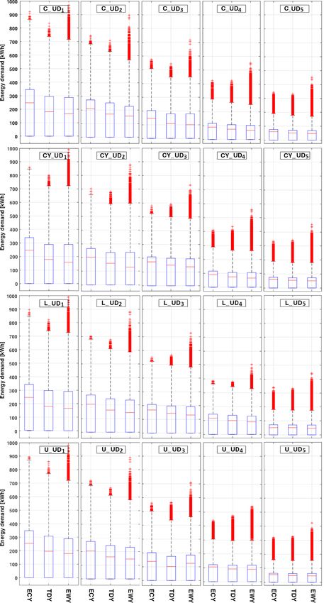
A.T.D. Perera et al. Applied Energy 285 (2021) 116430
Fig. 5. Twenty generated urban morphologies based on the BMC technique with their physical characteristics.
function of each building. To account for wind speed variations, the with the building renovation level. However, considering urban
verified model in the previous works of authors [54,55,70] have been morphology adds a level of complication since urban morphology
adopted based on BMC technique. changes bring notably affect the demand profile, which cannot be simply
presented using linear programming.
5. Co-optimization of urban morphologies and energy system
5.1. Optimization algorithm
A typical formulation of energy system optimization maps the deci
sion space variables that correspond to the energy system design to the
Bringing energy system design and urban form into the optimization
objective space through a time series simulation. This can be formulated
process entails formulating non-linear and non-convex objective func
in a deterministic, stochastic, robust, or stochastic-robust way. Irre
tions, for which linear/mixed-integer linear programming techniques or
spective of the method used, design parameters of the energy system and
a gradient-based technique are unsuitable. The direct influence of urban
dispatch variables are considered in the decision space. Both single and
form on the energy demand makes it difficult to decouple the optimi
multi-level optimization algorithms have been introduced to optimize
zation process into two levels where heuristic methods with linear
distributed energy systems. For example, Wang and Perera [56] intro
programming techniques can be used as introduced by Wang and Perera
duced a multi-level optimization algorithm that can design distributed
[56]. Hence, heuristic methods are used in this study as the optimization
energy systems along with the connected network while maintaining n-1
technique. The decision space vector presents the variables related to the
security. Evins [57] introduced a bi-level optimization algorithm where
energy system configuration, dispatch strategy and energy demand.
the dispatch strategy of the distributed energy system is optimized at the
System configuration defines the size of system components such as PV
primary level while system design is optimized at the secondary level. In
panels, wind turbines, battery bank, etc. Dispatch strategy defines the
general, multilevel optimization algorithms are computationally exten
fuzzy and finite-state transition rules. Energy demand is determined by
sive. For example, the optimization algorithm introduced by Evins [57]
two decision space variables corresponding to urban form and density.
takes several days to arrive at the optimal solution. Therefore, a single
The entire set of variables amounts to 30, which is a considerable
level optimization algorithm is used in this study. Single level optimi
number to be handled by a heuristic algorithm. Net Present Value of the
zation algorithms have been used previously to optimize the design of
system and grid integration levels are considered as objective functions
energy systems. Further, Wu et al. [58] used a single level optimization
while power supply reliability is used as a constraint in the optimization.
algorithm to determine optimal building energy system design along
The constraint tournament method [59] is used to consider the
7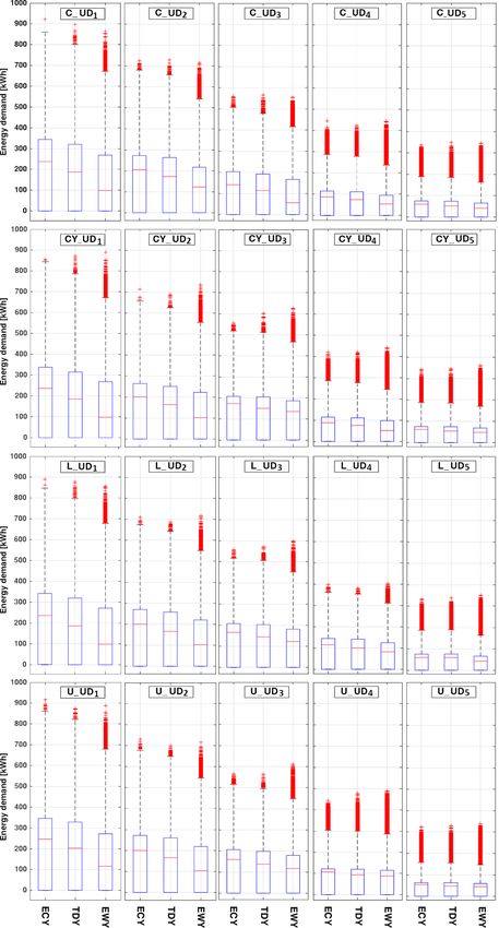
A.T.D. Perera et al. Applied Energy 285 (2021) 116430
constraint function during the optimization. A co-operative co-evolu irradiation on the tilted PV panel and the efficiency of the SPV panel.
tionary algorithm (COCE) often used to consider very extensive decision The Durisch model [64] is used to compute the efficiency of the PV
spaces is used to conduct the optimization. The co-evolutionarily algo panel. The model considers the global solar irradiation on the tilted SPV
rithm enables partitioning the decision space while cooperativeness panel, cell temperature, and air-mass as the inputs to the model when
enables considering non-variable separable problems along with the computing the efficiency of the PV panels. APV [ m2] and xpv denotes the
partitioning of the decision space variables. An extended explanation is area of the solar panel and number of PV panels installed, which is
presented in [60]. optimized in the optimization algorithm. Complexities inherent to city
morphologies make it difficult to consider the impact of shading, espe
5.2. Outline of the energy system cially when performing energy system sizing. We introduce a shading
factor ςPV to account for the losses due to shading. A similar approach is
An energy hub model introduced by Guidl and Anderson [61], which used to compute the power generation using wind turbines Eq. (2).
has been widely used during recent studies, is adopted in this work to
represent the energy system. Solar PV panels and wind turbines are PW ̃W w w
t = Pt (vt )x ς , ∀t ∈ T (2)
considered as non-dispatchable energy technologies. An internal com W
In Eq. (2), P
̃ (v ) [kWh] denotes the power generation from a single
bustion generator (ICG) is used as the dispatchable energy source. A t t
wind turbine. xw represents the number of wind turbines which is
battery bank is considered as energy storage. The heating and cooling
optimized using the computational model. Wind speed will be dropped
demand of the buildings is assumed to be catered by the heat pumps and
due to the urban boundary layer and losses in power converters are
air conditioners. The energy hub interacts with the grid when catering
represented byςw in the system (which is obtained using the optimiza
the fluctuating energy demand of the buildings. Grid curtailments are
tion algorithm) and the power losses. Power generation from the dis
considered when injecting the excess generated as well as buying elec
patchable sources, energy interactions with the grid, and energy storage
tricity from the grid. The hourly pricing scheme is considered for both
are determined by the dispatch strategy. The state of the charge model is
selling and purchasing electricity to and from the grid.
used to determine the charge level of the battery bank while the poly
nomial power curve is used to determine the fuel consumption of the
5.3. Dispatch strategy dispatchable energy source.
Dispatch strategy stands for the energy management strategy
implemented in the energy system to withstand the variations in energy 5.5. Formulation of objective functions and constraints
demand, renewable energy generation and grid conditions. The dispatch
strategy determines the optimal use of energy storage and can be pre Interactions with the grid are maintained within bounds. Grid cur
sented in different ways when conducting energy system optimization. A tailments are introduced for injecting and purchasing electricity to and
number of different methods have been used to implement a dispatch from the grid. Grid curtailments act as the primary barrier, which gua
strategy in energy system optimization. Bi-level optimization has often rantees smooth operation of the grid while accommodating renewable
been used to link dispatch and system optimization problems. Rule- energy technologies at a large scale. As the study focuses on autonomous
based models, grey-box models and reinforcement-learning algorithms energy districts, dependence on the grid is be minimized. Less depen
have been used to implement the dispatch strategy in the energy system dence on the grid encourages integrating more renewable energy tech
optimization problem. Although reinforcement learning can perform nologies within the district while helping to maintain the stability of the
exceptionally well concerning complex energy systems, it demands grid. In most of the instances, the grid acts as virtual storage when
much higher computational time and resources [60]. Therefore, the grey integrating renewable energy technologies, taking the excess generation
box model is considered in this study. A bi-level dispatch strategy is used within the micro-grid while supporting the catering of the energy de
in the grey box model [62]. The primary level is based on fuzzy mand whenever renewable energy generation is not sufficient. Support
automata, where operating conditions of the ICG are determined based from energy storage and dispatchable sources is required to balance the
on the mismatch between energy demand and renewable energy gen difference between demand and generation, which will add an addi
eration, state of charge in the battery bank and price of electricity in the tional cost to the system, creating a Pareto front between cost and the
grid. The secondary level uses finite state automata to derive the energy autonomy level of the district. Therefore, cost and autonomy level are
interactions between grid and energy storage. The energy interactions considered as the objective functions. Grid integration level is used as a
are determined considering the price of electricity in the grid, the state representative of the autonomy level. Lower grid integration levels will
of charge of the battery bank, and grid curtailments. A more compre lead to a higher autonomy level. Grid integration level is defined in this
hensive definition of the state space of the dispatch strategy is presented study according to Eq. (3) [62].
∑ ∑
in Ref. [63]. GI = EtIG / EtD (3)
∀t∈T ∀t∈T
5.4. Co-optimization of the energy system and urban form In this equation, EIG t [kWh] and Et [kWh] denote energy imported
D
from the grid and energy demand of the hub. The energy demand curve
A detailed energy flow model is used in this study, linking the urban is strongly influenced by the urban morphology. Hence, certain mor
simulation model with the energy system model. Energy demand on an phologies would lead to maintaining minimum interactions with the
hourly scale is fed into the energy system model, which depends on the grid. This makes it important to optimize the archetype along with the
urban morphology. Hourly power generation using Solar PV panels and system components.
wind turbines is computed subsequently. Power generation from the PV The net present value of the system represents the financial feasi
panels and wind turbines depends on hourly global solar irradiation on bility. Initial capital cost (ICC) of the system components as well as the
the tilted solar PV panel surface and wind speed at the wind turbine hub operation and maintenance costs are considered under the net present
level as well as installed capacities of these technologies. For example, value. Initial capital cost represents the acquisition and installation cost
renewable power generation using solar PV panels (PPV t ) for time step t is of system components such as PV panels, wind turbines, battery bank,
computed using Eq. (1). etc. The expenditure of constructing the building stock is not considered
PPV = Gβt ηPV PV PV PV
(1) in this study. Operation and maintenance costs consist of variables as
t A x ς , ∀t ∈ T
well as fixed operation and maintenance costs. Fixed operation and
t
In this equation, Gβt [kWh/m2] and ηPV
t denote the global solar maintenance costs (OMFixed c,s ) [EUR] consider regular annual expendi
8
A.T.D. Perera et al. Applied Energy 285 (2021) 116430
LPSt = EtD − PW PV ICG Bat−
t − Pt − PMax − Pt,s
Max
− IGLim , ∀t ∈ T (5)
In Eq. (5),PBat−t,s
Max
, IGLim , PICG
Max , ELDt,s [kWh] denote maximum
possible power flow from the battery bank (depends on the state of
charge), maximum power purchased from the grid, nominal power of
the internal combustion generator and electricity load demand. LOLP is
computed using Eq. (6)
∑
∀t∈T LPSt,s
LOLP = ∑ D
(6)
∀t∈T Et
6. Results and discussion
Energy requirements in the urban context can be influenced by both
urban morphology and climate conditions, which can notably influence
the design as well as the operation of distributed energy systems. A
comprehensive quantification of the influences brought by urban
morphology and climate variations can lead to improving energy effi
ciency as well as sustainability from the generation perspective. To
wards this objective, Section 6.1 presents the influence of urban climate
and urban morphology on the energy demand while Section 6.2 quan
tifies the impact of both these sectors while simultaneously optimizing
the energy system and urban morphology.
6.1. Impacts of urban morphology on energy demand
Results in this section help to understand how the energy demand
profiles (summation of heating, cooling, lighting, and appliance de
mands) alter based on the considered urban morphology. Distributions
of the hourly values of energy demand over one year (for typical and
extreme weather conditions) are shown in Fig. 6 using boxplots. The
values are presented for all twenty urban morphologies during
2010–2039, categorized according to major influencing parameters
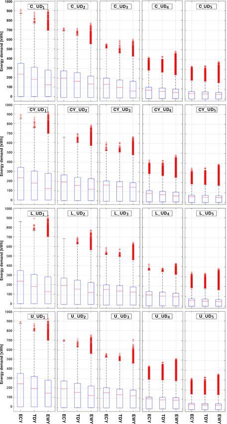
including building form and urban density. A similar comparison is
made for 2039–2069 and 2070–2099 in Figs. A1 and A2, available in the
Appendix.
As is visible in Fig. 6, a downward trend can be noticed, in which a
higher urban density results in higher energy demand. The difference in
the average annual energy demand for typical and extreme weather
conditions varies for each building form and urban density (UD1 to
UD5). For example, for the C-form buildings, the highest energy demand
on an annual scale is observed in ECY; where the average absolute dif
Fig. 6. Boxplot of annual energy demand for all urban morphologies based on ference between ECY and EWY is +20, +19, +17, +14, and +13 percent
UDs and forms (2010–2039). for UD1 to UD5, respectively. The lowest difference between average
annual energy demand for ECY and EWY is observed in the L-form
tures of maintaining system components and grid interactions. Variable buildings in UD5 with +9 percent; which clearly indicates the impacts of
urban morphology on the energy performance of buildings with similar
operation and maintenance costs (OMvariable
c ) [EUR] consider replace
building forms in extreme weather conditions.
ment cost for the dispatchable energy source and battery bank
An important part of the assessment is to quantify the impacts of each
depending upon the usage. Finally, the Net present value of the system is
UD (with similar built density, conditioned volume, and the number of
computed according to Eq. (4)
∑ ∑∑ floors) on the annual distribution of energy demand. Fig. 7 compares the
NPV = ICC + Fixed
(OMc,s CRFc )+ PRI l OMc,h,s
variable
, ∀t ∈ T, ∀c cumulative distribution of the annual energy demand for all the building
∀c∈C ∀h∈H ∀c∈C forms over three time periods with typical and extreme weather data
∈ C, ∀h ∈ H (4) sets. The CY-form buildings have the best performance in ECY for all the
urban morphologies, except for UD2 and UD3 where U- and C-form
In Eq. (4), CRFc denotes the Capital Recovery Factor for the cth
buildings have the lowest energy demand on an annual basis. Similar
component. PRI denotes the real interest rate calculated using both in
distributions can be observed in EWY for CY-form buildings in UD1, UD2,
terest rates for investment and the local market annual inflation ratio.
and UD4; while in UD 3 and UD 5 the U- and L-form buildings have a
The year considered is represented by h.
notably lower energy demand. For example, in UD1 (Aa = 13824 m2),
In addition to the two objective functions considered for the Pareto
CY-form have the best performance with average energy demand of
optimization, Loss of Load Probability (LOLP) is considered as a
211.8, 197.4 and 175.1 kWh in ECY, TDY and EWY; while L-form
constraint in the optimization process. LOLP has often been considered
buildings showed about 9%, 8% and 5% higher energy demand
to represent the power supply reliability [65–68].
respectively.
The loss of power supply (LPS) of the system is computed according
Table 1 shows the average energy demand for all urban morphol
to Eq. (5).
ogies based on building form and UDs. There is an upward trend during
9A.T.D. Perera et al. Applied Energy 285 (2021) 116430
Fig. 7. Cumulative energy demand for all urban morphologies based on UDs and forms for ECY, TDY and EWY (2010–2039, 2040–20069, and 2070–2099).
the second and third time period (2040–2069 and 2070–2099), where To assess the impacts of urban density and building form on the
energy demand of all urban morphologies increases by time except for energy demand profiles, the annual energy demand values per square
TDY. This upward trend coincides with the increment of average hourly meter are compared in Fig. 8. The lowest annual energy demand for ECY
air temperature in ECY and EWY weather datasets. For example, the and EWY conditions is observed in UD5 for all building forms. For
annual average energy demand in 2010–2039 increases by + 3 (7 kWh), example, in C-form buildings, the annual energy demand for UD1 to UD4
− 4.7 (10.2 kWh), and + 17 (26.8 kWh) percent adopting ECY, TDY, and is 10, 19, 10, and 11 percent higher than UD5 with 100.4 kWh/m2 en
EWY in 2069–2099. Similar to UD1, the average annual energy demand ergy demand in EWY. A similar condition is observed for ECY; where
increases in EWY for all BMCs (on average + 14 percent higher demand annual energy demand difference for UD1 to UD4 is +18, +27, +14, and
in 2070–2099 compared to the 2010–2039 time-period). +6 percent compared to UD5 with 117.3 kWh energy demand. For TDY,
10A.T.D. Perera et al. Applied Energy 285 (2021) 116430
Table 1
Average energy demand for all building forms in each UD.
Urban morphologies Building forms Energy demand [kWh]
2010–2039 2040–2069 2070–2099
ECY TDY EWY ECY TDY EWY ECY TDY EWY
UD1 C 220 200.7 175.9 224.7 192 190.5 227 190.8 205.1
CY 211.8 197.4 175.1 215.6 189.9 191.4 218.1 189.3 205.8
U 216.1 200.6 177.9 221.3 192.5 193.4 223.1 192 208.5
L 227.4 207.9 181.6 231.7 199.5 195.1 234.4 197.7 208.4
UD2 C 189.5 174.3 153.1 193.3 167.7 162.6 195 166.5 171.8
CY 172.9 164.4 149.5 175.3 159.5 162.5 178.1 160 173.3
U 180.3 167.5 148.9 183.7 161.6 160.6 185.4 160.9 171.8
L 183.2 168.5 148.4 186.9 161.9 159.2 188.8 160.7 169.6
UD3 C 135 125.2 111.6 138.1 120.3 121.1 139.8 119.7 131.8
CY 151.2 147.1 135.2 154.4 144 144.2 154.9 144 149.9
U 148.2 141.9 129.2 151 138.3 138.3 151.9 137.9 145.2
L 147 132.8 130.9 149.3 132.3 138.6 137.3 122 138.6
UD4 C 92.5 87.9 79.5 95 84.6 85.2 95.6 84.1 92.3
CY 90.9 86.8 78.8 93.1 83.7 85.3 93.9 83.5 92.5
U 101.7 96.7 87.3 104 94 93.7 104.4 93.6 98
L 107.8 106 99.9 110.5 103.4 105.5 110.8 103.2 111.2
UD5 C 69.4 65.7 59.5 71.4 63.1 63.5 71.7 62.7 69.1
CY 69.8 67.6 62.5 71.6 65.2 66.9 71.8 65.2 72.4
U 67.6 69.6 59.7 69.7 65.1 64.2 62.9 62.6 70
L 64 62.6 58.3 66.4 60.4 62.2 66 60.3 67.3
Fig. 8. Annual energy demand in kWh/m2for all urban morphologies based on the UDs and forms for ECY, TDY, and EWY (2010–2039, 2040–20069,
and 2070–2099).
these numbers are +14, +23, + 11, +0.1 percent indicating a similar Another important part of the assessment is comparing the impact of
trend. The highest annual energy demand in ECY for CY-, L-, and U-form urban morphology on the peak energy demands during typical and
buildings is observed in UD3 with 149.9, 146.9, 145.8 kWh/m2 extreme weather conditions (Fig. 9). The highest peak demand in all UDs
respectively. The highest annual energy demand overall observed in and building forms occurs in EWY, except for the U-form buildings in
UD4 (138.8 kWh/m2) using EWY weather dataset. Similarly, the energy UD1 whose highest peak demand is observed in ECY. The magnitude of
demand of all urban morphologies shows the highest increment by time peak demand increases notably by time in all UDs for EWY. It reaches
with up to 17 kWh/m2. It is interesting to mention that this increment is over 1073 kWh during 2070–2099 for the U-form buildings in UD1,
even higher in L-form urban morphologies. This is why C- and CY-form which is 25% more than the value for 2010–2039. Urban morphologies
buildings with more compact geometries and semi-courtyard spaces with C- and CY-form buildings showed a lower magnitude of peak en
show a better performance; particularly during warm seasons. ergy demand in all UDs. According to the results, energy demand in EWY
11A.T.D. Perera et al. Applied Energy 285 (2021) 116430
Fig. 9. Peak energy demand for all urban morphologies based on UDs and forms for ECY, TDY, and EWY (2010–2039, 2040–2069, and 2070–2099).
case of extreme climate events. To quantify the impact of urban
900 Urban form morphology on the energy system, the energy system is optimized
U considering the sensitivity of building form, urban density, and both
L these aspects together, as presented in Sections 6.2.1 and 6.2.2 respec
NPV per unit floor area (Euro/m2)
800
CY tively. Subsequently, the impact of extreme climate conditions on en
C
700 ergy system design is investigated in Section 6.2.3.
600 6.2.1. Sensitivity of building form
To understand the impact of building form on energy systems, a
500 Pareto optimization is conducted for each building form considering the
density of UD3, taking demand profiles for the 2010–2039 period.
400 Although the Pareto fronts do not show a significant difference in NPV
(Net Present Value), a noticeable split is observed in two groups
300 (Fig. 10). L and CY can be grouped into one class, which shows a rela
tively lower cost compared to the groups of U and C. The difference in
200 cost is not distinguishable when the grid interactions are low. The Pareto
0 500 1000 1500 2000 2500 fronts almost coincide when reaching the standalone operation mode.
Grid integration level (kWh/m2) The difference in cost is kept within 10% throughout the Pareto front,
which indicates that it closely follows the results of the building simu
Fig. 10. Pareto fronts obtained for different building forms considering the
lation where annual energy demands are kept within a 10% bound. This
same urban density.
indicates that the changes observed in annual demand does not reflected
in the Pareto fronts.
conditions will increase notably in all urban morphologies due to the
impacts of climate change on the variations of air temperature. This will 6.2.2. Sensitivity of urban density
considerably affect the energy system design for the future conditions The influence of urban density is clearly visible in both annual and
and mitigate the larger and more frequent average and peak demands peak energy demands as discussed in Section 6.1. To understand the
for each UD. influence of urban morphology on energy systems in a more holistic
manner, the sensitivity of energy systems to urban density must be
considered. Towards this objective, the energy system is optimized
6.2. Effect of urban morphology on the energy system
along with the urban form while maintaining the building form
(building form C). As is visible in Fig. 11 (a), a notable difference in cost
The impact of urban morphology can easily go beyond the energy
is observed when changing the urban density. For example, cost per unit
demand and influence energy system operation, which might be vital in
Fig. 11. Pareto front/s obtained considering (a) NPV and Grid integration level for different urban densities taking building form C and (b) entire decision space
including building form and urban densities.
12A.T.D. Perera et al. Applied Energy 285 (2021) 116430
TDY 2040
700 Ext. 2040-2069
Ext. 2070-2099
NPV per unit floor area (Euro/m2)
600
500
400
300
0 500 1000 1500 2000
Grid integration level (kWh/m2)
Fig. 12. Variation of Levelized Energy Cost (LEC) along with levelized grid Fig. 13. Pareto fronts obtained considering typical and extreme
integration level for the Pareto solutions. climate conditions.
area can increase by more than 50% when moving from UD5 to UD1. compared to the morphologies with a lower urban density. There are
Such a significant change in the objective function values easily results significant drops in part-load efficiencies at lower operating lead factors,
in a significant change in the required energy system design. When diminishing the advantage obtained from the scale of economy. As a
analyzing the five Pareto fronts, a higher density will lead to a higher result, LEC values coincide with all the Pareto solutions when grid
cost per unit area except for UD3. A significant shift in the objective integration levels are low. As the LEC is similar for all the densities and
function values can be observed when moving from one density class to UD1 and UD2 have a much higher demand, the cost of UD1 and UD2 is
another. UD1-3 shows a gradual reduction in cost with the increase of high when compared to UD5 in Region A. However, the levelized gen
grid integration level while UD5 presents a notable reduction in cost eration cost notably decreases for both UD1 and UD2 compared to UD5,
when the grid integration levels are low in contrast to other urban which compensates the higher energy demand. As a result, the NPV per
densities. However, the drop-in cost gradually diminishes with the in unit area is low for UD5 when grid interactions are lower (Region A),
crease of grid integration level. By contrast, UD1-3 maintains the drop in while UD2 presents a lower NPV per unit area when the grid interactions
cost even after the grid integration level reaches beyond the 1250 kWh/ are high. This leads us to understand the Pareto front obtained,
m2 limit as shown in Region B. More importantly, UD1-5 reach lower considering the full decision space including energy system configura
NPV values when compared to UD5 in Region B especially towards the tion, urban density, and building form as presented in Fig. 11 (b).
end of the Pareto fronts. This analysis makes it easier to understand the
complete Pareto front considering both system configuration and urban 6.2.3. Sensitivity of energy systems to climate variations
morphology as presented in Fig. 11 (b). As discussed in Section 6.1, climate change notably influences the
It is interesting to investigate the reasons for the cost per area energy demand of buildings. Typical demand profiles consider the
increasing with urban density. The higher cost may occur due to1) gradual changes in the demand profile but not extremes while ECY and
higher energy demand in buildings, and 2) higher cost in catering to the EWY do consider extremes. An increased average temperature will result
demand. Table 1 provides a clear explanation for the first hypothesis. It in a higher cooling demand on average while stronger extreme events
is clear that certain urban forms are more energy-efficient than the will increase the peak energy demand. In this section, the sensitivity of
others, both for annual and peak energy demands. This clearly explains the energy system to climate variations (considering both long- and
why UD5 leads to a lower cost per unit area when compared to the short-term variations) is discussed. Pareto fronts obtained in previous
others. However, the analysis of the energy demand does not explain the sections are derived considering the typical energy demand as explained
behavior of the Pareto fronts in Region B, which leads us to the second in Section 3, which is the usual practice. Rising temperatures put
point (performance of the energy system and higher cost in demand building HVAC systems under strain by increasing the energy demand
catering). In Fig. 12 the Levelized Energy Cost (LEC) is plotted against especially during extreme climate events such as heatwaves. Consid
the levelized grid integration, which provides an overview of the cost of ering such extreme climate conditions will be vital in the future, espe
generating energy units for each Pareto solution for the five Pareto cially with a larger penetration level of renewable energy sources and
fronts. When analyzing the LEC of the Pareto solutions it is clear that all limited availability of backup dispatchable generators based on fossil
the design solutions show similar LEC when grid interactions are at a fuels. Hence, Pareto optimization is performed for urban density UD5
minimum level. However, the gap between the Pareto fronts becomes under typical and extreme climate conditions. A significant increase in
noticeable when increasing the grid interaction levels. The morphol NPV by up to 40% (Fig. 13) is observed when moving from a typical
ogies with higher urban density become more economical when scenario to extreme conditions. The increase in cost that is observed in
compared to the morphologies with a lower urban density. For example, energy infrastructure goes well beyond the annual energy demand in
the LEC decreases from 0.17 to 0.12 Euros when moving from UD5 to crease for extreme climate events. This clearly reflects the magnifying
UD1 within Set A, reducing the cost by 45%. UD1 caters a much larger effect of climate impact with regard to extreme climate events when
energy demand when compared to UD5, which leads to generating en shifting focus from the building sector to the energy sector.
ergy at a much cheaper cost due to the scale of the economy. This ex
plains that LEC decreases with an increasing grid integration level. 7. Conclusions
However, when reaching standalone conditions the energy system that
caters denser morphologies needs to work harder, since morphologies The present study extends the scope of the present state of the art by
with higher urban density need to cater higher peak demands when considering the influences of urban morphology on energy generation,
13You can also read