The effect of univariate bias adjustment on multivariate hazard estimates - Earth System Dynamics
←
→
Page content transcription
If your browser does not render page correctly, please read the page content below
Earth Syst. Dynam., 10, 31–43, 2019
https://doi.org/10.5194/esd-10-31-2019
© Author(s) 2019. This work is distributed under
the Creative Commons Attribution 4.0 License.

                     The effect of univariate bias adjustment on
                            multivariate hazard estimates
                               Jakob Zscheischler1,2,3 , Erich M. Fischer1 , and Stefan Lange4
       1 Institutefor Atmospheric and Climate Science, ETH Zurich, Universitaetstrasse 16, 8092 Zurich, Switzerland
              2 Climate  and Environmental Physics, University of Bern, Sidlerstrasse 5, 3012 Bern, Switzerland
                 3 Oeschger Centre for Climate Change Research, University of Bern, 3012 Bern, Switzerland
                  4 Potsdam Institute for Climate Impact Research (PIK), Member of the Leibniz Association,

                                          P.O. Box 60 12 03, 14412 Potsdam, Germany
                          Correspondence: Jakob Zscheischler (jakob.zscheischler@climate.unibe.ch)

                               Received: 7 September 2018 – Discussion started: 13 September 2018
                      Revised: 23 November 2018 – Accepted: 26 November 2018 – Published: 7 January 2019

       Abstract. Bias adjustment is often a necessity in estimating climate impacts because impact models usually
       rely on unbiased climate information, a requirement that climate model outputs rarely fulfil. Most currently used
       statistical bias-adjustment methods adjust each climate variable separately, even though impacts usually depend
       on multiple potentially dependent variables. Human heat stress, for instance, depends on temperature and rel-
       ative humidity, two variables that are often strongly correlated. Whether univariate bias-adjustment methods
       effectively improve estimates of impacts that depend on multiple drivers is largely unknown, and the lack of
       long-term impact data prevents a direct comparison between model outputs and observations for many climate-
       related impacts. Here we use two hazard indicators, heat stress and a simple fire risk indicator, as proxies for
       more sophisticated impact models. We show that univariate bias-adjustment methods such as univariate quantile
       mapping often cannot effectively reduce biases in multivariate hazard estimates. In some cases, it even increases
       biases. These cases typically occur (i) when hazards depend equally strongly on more than one climatic driver,
       (ii) when models exhibit biases in the dependence structure of drivers and (iii) when univariate biases are rel-
       atively small. Using a perfect model approach, we further quantify the uncertainty in bias-adjusted hazard in-
       dicators due to internal variability and show how imperfect bias adjustment can amplify this uncertainty. Both
       issues can be addressed successfully with a statistical bias adjustment that corrects the multivariate dependence
       structure in addition to the marginal distributions of the climate drivers. Our results suggest that currently many
       modeled climate impacts are associated with uncertainties related to the choice of bias adjustment. We conclude
       that in cases where impacts depend on multiple dependent climate variables these uncertainties can be reduced
       using statistical bias-adjustment approaches that correct the variables’ multivariate dependence structure.

1   Introduction                                                   thus require unbiased climate information as input. However,
                                                                   biases continue to persist in global (Flato et al., 2013; Wang
With ongoing climate change, climate impact modeling has           et al., 2014) and regional climate models (Christensen et al.,
become an important pillar of climate research, informing          2008; Kotlarski et al., 2014), rendering bias adjustment an
decision makers and risk managers in many sectors that are         undesired but often unavoidable data processing step for cli-
affected by climate variability. Impact models such as hy-         mate impact modeling (Piani et al., 2010).
drological models, crop models and epidemiological models             The need for easily available information on climate im-
usually rely on absolute thresholds in their driving climate       pacts has led to a sometimes overly uncritical use of bias
variables such as temperature, precipitation, wind speed and       adjustment in large impact modeling projects, even though
humidity (Winsemius et al., 2015; Ruane et al., 2017); and

Published by Copernicus Publications on behalf of the European Geosciences Union.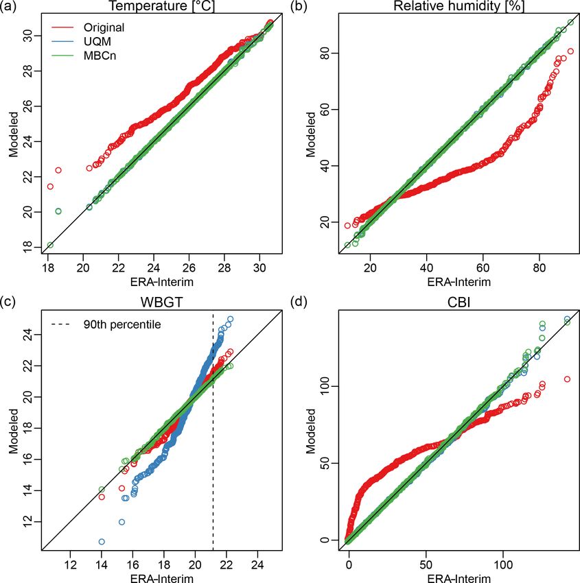
32                          J. Zscheischler et al.: The effect of univariate bias adjustment on multivariate hazard estimates

its current usage might, in some cases, result in ill-informed      variate bias-adjustment methods have been suggested in the
adaptation decisions (Maraun et al., 2017). It is often as-         recent past (Piani and Haerter, 2012; Li et al., 2014; Vrac
sumed that biases are stationary, and hence that bias adjust-       and Friederichs, 2015; Cannon, 2016; Mehrotra and Sharma,
ment can be developed in the current climate and applied in         2016; Vrac, 2018). In addition to adjusting the marginal dis-
a warmer world. It is not clear, however, for which variable        tributions, these methods adjust, to a certain extent, the de-
and to what extent this assumption is met. Moreover, while          pendence structure between multiple variables. Some stud-
uncertainties related to the choice of climate model and im-        ies have recently suggested that multivariate approaches do
pact model as well as future socioeconomic scenarios are            not lead to a substantial improvement for certain specific re-
frequently carried through the modeling chain (Wilby and            gional impacts (Yang et al., 2015; Casanueva et al., 2018;
Dessai, 2010; Frieler et al., 2017), uncertainties associated       Räty et al., 2018). However, this does not imply that multi-
with the choice of the applied bias-adjustment method are           variate bias adjustment is not necessary in any case. Many
rarely reported (Ehret et al., 2012), though there are excep-       multivariate methods have not been systematically evaluated
tions (Chen et al., 2011; Bosshard et al., 2013; Addor and          against modeled impacts and have been rarely used in larger-
Fischer, 2015).                                                     scale impact modeling frameworks, though there are notable
   Assessing the appropriateness of bias adjustment for im-         exceptions. For instance, Cannon (2018) presents a highly
pact modeling is not an easy task (Papadimitriou et al., 2017).     flexible multivariate bias-adjustment method and demon-
While the quality of bias adjustment on climate variables can       strates its effectiveness on a modeled multivariate hazard in-
be evaluated against observed quantities in the climate do-         dicator. By adjusting biases and dependencies between tem-
main, the implications for modeled impacts are much harder          perature, precipitation, relative humidity and wind speed, the
to determine. On the one hand, limited length and a lack of         method substantially reduces biases in the five-dimensional
homogeneity in observed climate impacts render an evalu-            Fire Weather Index (FWI), outperforming univariate bias-
ation of modeled impacts very challenging (Cramer et al.,           adjustment approaches.
2014). On the other hand, many impacts rely on the com-                In this paper we study the limitations of univariate bias-
plex interaction of multiple climate variables across time and      adjustment methods for multivariate impacts. We focus on
space (Zscheischler et al., 2018), preventing an evaluation         global-scale climate outputs from global circulation models
in the climate domain. For instance, temperature and pre-           (GCMs), which are frequently used for global impact stud-
cipitation variability affect crop yields (Semenov and Porter,      ies (Winsemius et al., 2015; Frieler et al., 2017; Ruane et al.,
1995; Zscheischler et al., 2017) and other ecosystem services       2017). However, our analyses are of a rather conceptual na-
such as net carbon uptake (Humphrey et al., 2018). Flood            ture and thus also apply to other climate model outputs, for
occurrence, its intensity and associated damages depend on          instance from regional climate models. First, we investigate
the temporal and spatial characteristics of precipitation, soil     whether traditional univariate bias-adjustment methods gen-
moisture, river flow and surge (Vorogushyn et al., 2018).           erally reduce biases in impacts that depend on multiple de-
Drought-related impacts depend on precipitation, evapotran-         pendent drivers. Bias adjustment may also amplify uncertain-
spiration, and temperature; their spatial distribution; and their   ties inherent to the observations (Chen et al., 2011). Hence,
interaction with human activities (Van Loon et al., 2016).          using a model environment with multiple models and mul-
Fire occurrence, and strength, not only requires available fuel     tiple runs for a single model, we further estimate how un-
and an ignition source, but is also strongly dependent on           certainties related to internal variability may be propagated
relative humidity and temperature (Brando et al., 2014). In-        and amplified through incomplete bias adjustment. We use
frastructural damage is particularly large when strong winds        multivariate hazard indicators as proxies for actual impacts
and extreme precipitation occur jointly (Martius et al., 2016).     to evaluate the effect of bias adjustment on impacts and to
Finally, climate-related human-health impacts are linked to         overcome the challenge of missing impact data. It can be as-
a suite of climatic drivers (McMichael et al., 2006). It is         sumed that “real” impacts are in many cases more complex
currently largely unknown how widely used statistical bias-         and also depend on more driving variables. Therefore, our
adjustment approaches affect modeled impacts that depend            analysis provides a rather conservative estimate of the poten-
on multiple drivers such as the ones mentioned above.               tial effects of univariate bias adjustment on modeled impacts.
   Bias-adjustment methods are often designed to correct one
variable at a time (Teutschbein and Seibert, 2012; Hempel
                                                                    2     Data and methods
et al., 2013). A possible bias in the dependence structure
between climate variables is therefore not adjusted, even           2.1    Data
though climate models may not capture dependencies be-
tween climate drivers very well, for instance the correlation       Observations. We use daily temperature and relative hu-
between temperature and precipitation in summer (Zscheis-           midity from the ERA-Interim reanalysis (Dee et al., 2011)
chler and Seneviratne, 2017). Even worse, correcting a bias         as main reference dataset. We further use daily tempera-
in marginal distributions may modify the dependence be-             ture and relative humidity from the observational dataset
tween variables. In recognition of these issues, several multi-     EWEMBI (Lange, 2016, 2018), which has been used in the

Earth Syst. Dynam., 10, 31–43, 2019                                                     www.earth-syst-dynam.net/10/31/2019/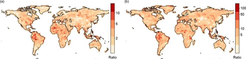
J. Zscheischler et al.: The effect of univariate bias adjustment on multivariate hazard estimates                                        33

Inter-Sectoral Impact Model Intercomparison Project phase
2b (ISIMIP2b; Frieler et al., 2017).
   Model simulations. We use daily model output from
the historical runs of the Coupled Model Intercomparison
Project Phase 5 (CMIP5; Taylor et al., 2012). A main objec-
tive of the CMIP5 model experiments is to improve our un-
derstanding of the climate system, and to provide estimates
of future climate change. All 29 model simulations used in
this study are listed in Table A1.
   All data have been bilinearly interpolated to a 2.5◦ by 2.5◦
regular latitude–longitude grid prior to analysis. The studied
time period is 1981–1995. Our analysis is based on daily val-
ues during the hottest month of the year at each grid point,
which results in about 450 samples. We focus on the hottest
month to avoid dealing with seasonality and because, ar-
guably, fire risk and heat stress are most relevant during this
time period. The hottest month was identified based on the
climatology of ERA-Interim monthly temperature data. Al-
though the effectiveness of bias adjustment is typically eval-
uated outside the calibration period (Maraun, 2013), here we
focus our analysis completely on the selected 15-year pe-
riod. This allows for a separate assessment of the effect of        Figure 1. Distribution of daily temperature versus relative humid-
bias adjustment on univariate versus multivariate impacts in-       ity during July (1981–1995) for a grid point in central Africa.
dependently from other effects such as cross-validation er-         ERA-Interim (a); model simulations from the model IPSL-CM5A-
ror. A good performance in the calibration period is a neces-       MR (b); bias-adjusted with UQM (c); bias-adjusted with MBCn (d).
sary requirement for an effective bias-adjustment approach.         Pink lines depict levels of equal heat stress (WBGT). Violet lines
Furthermore, cross-validation might not help to diagnose            depict levels of equal fire risk (CBI). Red points denote values for
whether a bias-adjustment approach is effective (Switanek           which WBGT exceeds its 95th percentile.
et al., 2017; Maraun and Widmann, 2018).
                                                                    2013), our goal here is rather to provide an illustrative exam-
2.2   Methods                                                       ple of the issues associated with bias adjustment and impact
                                                                    modeling than to provide the most reliable hazard projec-
Hazard indicators. We use the Wet Bulb Globe Temperature
                                                                    tions. We estimate WBGT following the approach outlined
(WBGT; Dunne et al., 2013) as an indicator for heat stress
                                                                    in the supplement of Dunne et al. (2013). CBI can be com-
and the Chandler Burning Index (CBI; Chandler et al., 1983)
                                                                    puted as
as an indicator for fire risk. Both are relatively simple indica-
tors that can be computed solely from daily temperature and         CBI =
relative humidity. WBGT and its variants have been exten-

                                                                          ((110 − 1.373 RH) − 0.54(10.2 − T )) 124 · 10−0.0142 RH /60,   (1)
sively used to assess projections of heat stress under climate
change (Pal and Eltahir, 2015; Zhao et al., 2015; Li et al.,        where RH is relative humidity in % and T is temperature in
2017). CBI is one of many fire risk indicators (Lee, 1980;          degrees Celsius.
Carlson and Burgan, 2003), mainly chosen here for its sim-             Bias adjustment. We employ two different bias-adjustment
plicity. The hazard intensities of WBGT and CBI vary along          methods, the widely used univariate empirical quantile map-
different gradients in the temperature–humidity domain (Fis-        ping (UQM; Panofsky and Brier, 1968; Maraun, 2013;
cher et al., 2013; Zscheischler et al., 2018). WBGT increases       Casanueva et al., 2018) and the multivariate bias adjust-
with hotter and more humid conditions and is equally depen-         ment in n dimensions (MBCn) developed by Cannon (2018).
dent on temperature and humidity (Fig. 1). In contrast, CBI         UQM applies separate corrections to a fixed number of quan-
increases with hotter and drier conditions and its variability      tiles to adjust a modeled empirical cumulative distribution to-
is mostly driven by humidity and much less by temperature.          wards the observed empirical cumulative distribution. Hence,
Using two hazard indicators that depend differently on the          if Xo and Xm are the observed and modeled values, respec-
same climatic drivers enables us to study how the relation-         tively, then
ship between hazard direction and driver distribution changes
                                                                    X̂m = Fo−1 (Fm (Xm )),                                               (2)
the way bias adjustment affects modeled hazards (Zscheis-
chler et al., 2018). While certainly more sophisticated indi-       where Fm is the empirical cumulative distribution function of
cators exist, both for fire risk and heat stress (Bröde et al.,     Xm and Fo−1 is the inverse empirical distribution function (or

www.earth-syst-dynam.net/10/31/2019/                                                           Earth Syst. Dynam., 10, 31–43, 2019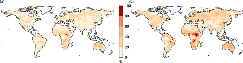
34                                 J. Zscheischler et al.: The effect of univariate bias adjustment on multivariate hazard estimates

quantile function) corresponding to Xo . Values between the
predefined quantiles are approximated using linear interpola-
tion. We apply UQM with the R package qmap (Gudmunds-
son, 2014) using 100 quantiles.
   MBCn is a bias-adjustment method in which both the
marginal distribution of each individual variable and the mul-
tivariate dependence structure are corrected at the same time
(Cannon, 2018). This is achieved by an iterative approach,
which first applies a random rotation R [j ] to the multivariate
observed and modeled data distribution
  [j ]    [j ]
X
em     = Xm R [j ] ,                                             (3)
eo[j ]
X
            [j ]
         = Xo R [j ] .                                           (4)

Subsequently, quantile mapping (Eq. 2) is applied to the ro-
             [j ]                                        [j ]
                       eo[j ] as a reference, yielding X̂m
tated data X
           em     with X                                      . Then
the inverse rotation is applied
  [j +1]        [j ]      −1
Xm         = X̂m R [j ]        .                                 (5)

The observed data are carried forward to the next iteration
               [j +1]     [j ]
unchanged Xo          = Xo . These steps are repeated until the         Figure 2. Quantile–quantile plot of observed versus modeled val-
modeled data distribution has converged to the observed dis-            ues for temperature (a), relative humidity (b), heat stress (WBGT, c)
tribution. One may interpret the algorithm such that the ran-           and fire risk (CBI, d) for a grid point in central Africa; original
dom rotations allow an information exchange between the                 model output (from IPSL-CM5A-MR) in red, model output cor-
different dimensions.                                                   rected with UQM in blue, model output corrected with MBCn in
   Finally, we use the bias-adjustment method (Lange, 2017)             green. The vertical dashed line in (c) shows the 90th percentile of
applied in ISIMIP2b (Frieler et al., 2017). This method ad-             observed WBGT. The same data as in Fig. 1 were used. Note that in
justs relative humidity with parametric quantile mapping us-            panels (a, b, d) the green circles cover most of the blue circles, as
                                                                        in these cases both bias adjustments yield virtually identical results.
ing beta distributions to model simulated and observed daily
values (Frieler et al., 2017; Lange, 2018), and temperature
with an additive correction of monthly mean temperature
                                                                        against each other to estimate the range of the uncertainty
and a multiplicative correction of daily anomalies from the
                                                                        due to internal variability (“noise”). Bias adjusting all other
monthly mean temperature (Hempel et al., 2013).
                                                                        model runs against all five CanESM runs then provides an
   We adjust daily values of temperature and relative humid-
                                                                        estimate for the full uncertainty range (“full range”). Com-
ity in CMIP5 during the hottest month at each grid point and
                                                                        paring the range of the noise with the full range, we esti-
evaluate the change in bias for WBGT and CBI.
                                                                        mate whether univariate bias adjustment amplifies uncertain-
   Perfect model approach. Internal variability can lead to un-
                                                                        ties related to internal variability.
certainties in the bias adjustment, which may be amplified
through an inadequate choice of bias adjustment. Since fully
coupled ocean–atmosphere models provide different realiza-              3   Results
tions of unforced internal variability, observations and mod-
els as well as different simulations of the same model are not          Statistical bias adjustment that is separately applied to each
expected to agree on a year-by-year basis. Even when using              marginal distribution of a multivariate distribution such as
a time period of 2–3 decades, this constitutes a substantial            UQM ensures that the bias-adjusted modeled marginal dis-
source of uncertainty (Addor and Fischer, 2015). Using the              tributions are well aligned with the observed marginal dis-
multimodel environment of CMIP5, we study whether UQM                   tributions. We illustrate the effect of bias adjustment for
increases uncertainties related to internal variability for mul-        one selected grid point in central Africa. UQM “squeezes”
tivariate hazard indicators. We conduct a perfect model ap-             and “stretches” a modeled multivariate distribution along the
proach to separate uncertainties associated with internal vari-         marginal axes to match the observations of the marginals
ability and the choice of bias adjustment (Griffies and Bryan,          (Fig. 1c). For hazards that are a function of multiple drivers
1997; Elía et al., 2002; Hawkins et al., 2011). To this end we          and that vary along a diagonal gradient such as WBGT, UQM
use the five available initial-condition members of the model           may not be able to reduce biases. In fact, for many per-
CanESM to estimate the influence of internal variability as             centiles, it can even increase biases as illustrated in Fig. 2c
a source of uncertainty. First, we bias-adjust CanESM runs              (blue dots). CBI seems to be less affected, likely because its

Earth Syst. Dynam., 10, 31–43, 2019                                                           www.earth-syst-dynam.net/10/31/2019/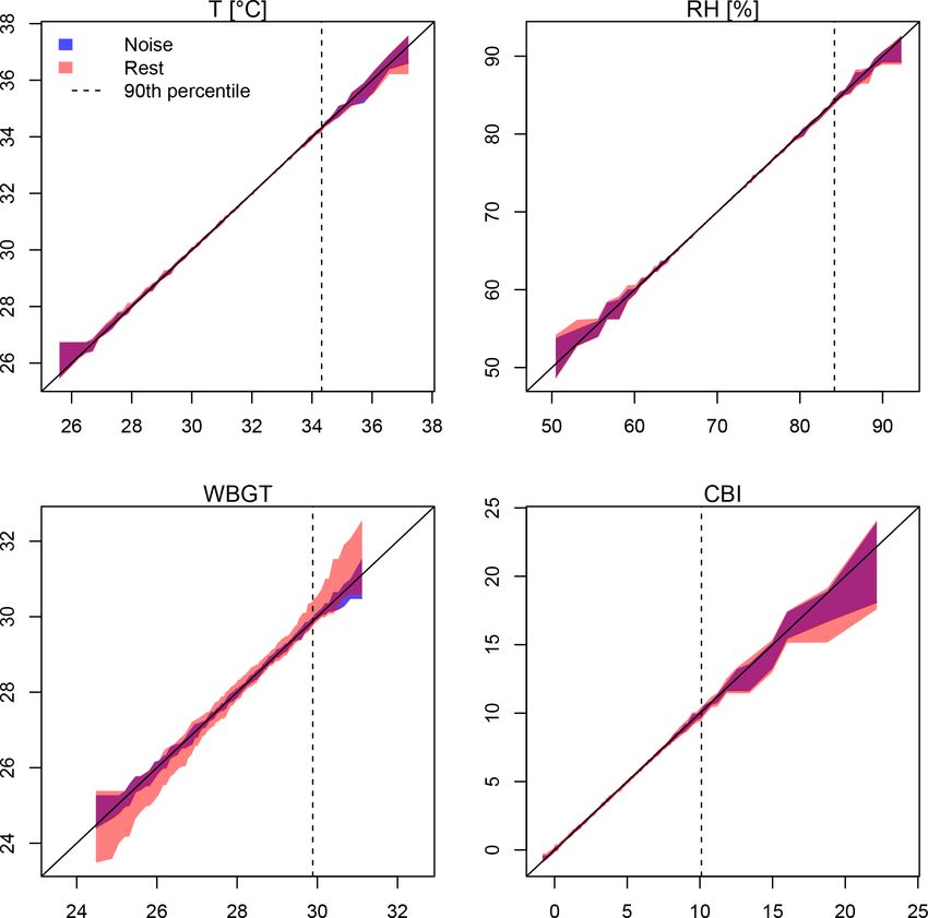
J. Zscheischler et al.: The effect of univariate bias adjustment on multivariate hazard estimates                                     35

Figure 3. Fraction of grid points for which UQM increases bias (a) or does not result in a reduction of more than 50 % in biases (b) of
modeled hazards. Box plots represent the CMIP5 multimodel ensemble after UQM and highlight the median (horizontal line), interquartile
range (box), 1.5 times the interquartile range (whiskers) and outliers (points). Colored dots represent the results for the ISIMIP2b bias
adjustment applied to the four GCMs used in ISIMIP2b. Shown are the metrics RMSE between empirical cumulative distribution functions
and absolute differences in the 90th (1q90) and 95th percentile (1q95) between hazard indicators computed from (bias-adjusted) model
outputs and observations (ERA-Interim for CMIP5 and EWEMBI for ISIMIP2b).

variability is mostly driven by a single variable, namely rela-        reach this benchmark (Fig. 3b). Note that this means that in
tive humidity (Figs. 1–2).                                             the majority of grid points, UQM reduces biases in WBGT.
   Bias adjustment can also affect the relationship between a          However, in many cases the reduction is not satisfactory. Un-
multivariate hazard indicator and its individual contributing          derstanding the conditions under which bias adjustment fails
climate variables. For instance, looking at the raw model out-         may help to design and use approaches that are more suitable
put of IPSL-CM5A-MR in Fig. 1b, one would infer that high              for the given target. In contrast to WBGT, for CBI, UQM ef-
heat stress (WBGT values exceeding their 95th percentile,              ficiently reduces the bias in most cases. Relative humidity
highlighted in red) is reached at rather low relative humidity.        alone explains most of the variance in CBI (Fig. 1); hence,
Instead, for ERA-Interim data for the same grid point, high            UQM can correct it very well (Figs. 2–3). If instead of UQM
heat stress is associated with high relative humidity (Fig. 1a).       the bias adjustment used in ISIMIP2b is applied, the num-
UQM improves this mismatch to some extent but not entirely             bers mostly fall into the CMIP5 range for WBGT (Fig. 3).
(Fig. 1c). Using MBCn for bias adjustment we would infer               However, for CBI, more grid points show no substantial im-
the correct contribution of individual variables. This is an im-       provement after bias adjustment compared to CMIP5. This
portant aspect, which needs to be taken into account when              is probably due to the fact that UQM is extremely flexible
applying bias adjustment because it may lead to incorrect              and thus almost perfectly adjusts temperature and relative hu-
conclusions about which climate drivers are most relevant for          midity. This in turn leads to a very good adjustment of CBI,
extreme hazards and impacts. Consequently, we might also               whose variability largely follows relative humidity (Fig. 1),
focus on the wrong aspects to improve in numerical climate             whereas the bias adjustment used in ISIMIP2b is more con-
models.                                                                servative and therefore less flexible in adjusting CBI.
   In the following, we quantify whether the case illustrated             Regions for which biases only slightly increase or decrease
in Figs. 1 and 2 is representative across the globe. We find           include locations where biases are small to start with. To
that an increase in root mean squared error (RMSE) be-                 study for how many grid points this is the case, we compute
tween the cumulative distribution functions of ERA-Interim             the fraction of grid points for which the bias in WBGT is
and model outputs before and after bias adjustment is an ex-           larger than 1 K either before or after bias adjustment. This is
ception (Fig. 3a). However, even though biases decrease at             the case for 50 %–90 % of the grid points, depending on the
most grid points when applying UQM, the reduction in bias              model and the metric (Fig. 4a). Recomputing Fig. 3 based on
is less than 50 % at 15 ± 6 % (mean ± one standard deviation           this subset reduces the fraction of locations where bias ad-
across models) of all grid points (Fig. 3b). Reducing biases           justment does not achieve the two benchmarks by about half
for extreme percentiles (≥ q90) may be even more challeng-             (Fig. 4b, c). Because these numbers strongly depend on the
ing. For instance, for the 90th (95th) percentile of WBGT,             size of the accepted bias (1 K in our example), we continue
UQM applied on temperature and relative humidity results               the analysis with all grid points.
in WBGT estimates that have larger biases than the estimate               In Australia, the Sahel, and some parts in sub-Saharan
based on raw model output for about 15 ± 6 % (18 ± 8 %) of             Africa and South America, UQM increases biases in the 90th
all grid points (Fig. 3a). If we ask for a reduction in bias by        percentile of WBGT for a large fraction of models (Fig. 5a).
at least 50 %, 27 ± 10 % (32 ± 12 %) of grid points cannot             In those regions, but also some other areas in the world,

www.earth-syst-dynam.net/10/31/2019/                                                          Earth Syst. Dynam., 10, 31–43, 2019
36                            J. Zscheischler et al.: The effect of univariate bias adjustment on multivariate hazard estimates

Figure 4. (a) Fraction of grid points for which biases in WBGT are larger than 1 K before or after the application of bias adjustment. (b–c)
As in Fig. 3 only for WBGT, based on the subset of grid points identified by (a).

Figure 5. Fraction of models for which UQM increases biases (a) or does not decrease biases by more than 50 % in the 90th percentile of
WBGT (b).

UQM reduces WBGT biases in the 90th percentile by less                      Internal variability can impact the effectiveness of bias ad-
than 50 % in the majority of all models (Fig. 5b). Overall,              justment because it introduces uncertainties that may be am-
in nearly 11 % of the land area, for more than 50 % of the               plified by incomplete bias adjustment. For temperature and
models, UQM does not reduce the bias of the 90th percentile              relative humidity individually, the perfect model approach
of WBGT by more than 50 %. MBCn, on the other hand, is                   reveals little difference between the range of the noise (un-
able to fit the hazard estimates well where UQM fails (not               certainty associated with internal variability) and the uncer-
shown for all grid points but Figs. 1d and 2c illustrate the             tainty range of all models (Fig. 7 illustrates the approach for
worst case).                                                             the grid point of Austin, Texas, US). This is to be expected,
   To improve the usage of bias-adjustment methods it would              as these driver variables can be perfectly adjusted. In the case
be important to know whether we can make any a priori                    of WBGT and CBI, however, UQM leads to much larger
statements as to whether UQM adjustment will lead to a                   uncertainties for the full range than for the noise for some
reduction in biases of modeled multivariate hazards or im-               percentiles (Fig. 7). Overall, the full range of bias-adjusted
pacts. Generally, regions where UQM fails to improve bi-                 model simulations for the 90th percentile of WBGT is a fac-
ases in WBGT coincide with regions where the observed                    tor of 10 larger than the range expected from internal vari-
correlations between temperature and relative humidity is                ability alone in many regions, including the Amazon, east-
outside the CMIP5 range (Fig. 6a). UQM fails when (uni-                  ern North America and Indonesia (Fig. 8a). The regions with
variate) mean biases in temperature are small (Fig. 6b), and             large increases in uncertainty roughly coincide with regions
when the correlation between the driving variables (in this              where the between-model variability in the correlation be-
case temperature and relative humidity) are not well captured            tween temperature and relative humidity is very high com-
(Fig. 6d). The mean bias in relative humidity looks similar              pared to the variability within the CanESM runs (Fig. 8b).
for both cases (Fig. 6c). Overall this means that if mean bi-            This is consistent with Fig. 6d, which shows that univariate
ases in climate drivers are large, any bias adjustment will lead         bias adjustment is not very successful when the correlation
to a substantial reduction in biases of hazard or impact indi-           structure between models and reference is not well matched.
cators (consistent with Fig. 4).                                         For a fixed percentile threshold, the fraction of grid points

Earth Syst. Dynam., 10, 31–43, 2019                                                           www.earth-syst-dynam.net/10/31/2019/
J. Zscheischler et al.: The effect of univariate bias adjustment on multivariate hazard estimates 37
Figure 6. Reasons why UQM may fail. (a) Regions in which the correlation between temperature and relative humidity in ERA-Interim is
outside the CMIP5 model range; (b–d) conditions where UQM does not lead to a substantial reduction in biases in WBGT (measured as
difference in empirical cumulative distribution function RMSE between model output and ERA-Interim before and after bias adjustment).
Shown is the mean bias in temperature (T , b) and relative humidity (RH, c) as well as the mean difference in correlation over all grid cells
between temperature and relative humidity (d). Blue (red) represents the distribution across models for cases in which UQM does (does not)
lead to a reduction in biases of WBGT by at least 50 %.
ity is largely indistinguishable from the full uncertainty range
(Fig. 9, dashed lines).
4 Discussion
We find that UQM of temperature and relative humidity often
does not lead to a substantial reduction in WBGT biases. In
a sizable number of cases UQM even leads to an increase in
the original biases, particularly for high percentiles that are
potentially most impact relevant. The fire risk indicator CBI
is less affected by these issues because, although temperature
is required for calculating it, it is largely dominated by vari-
ations in relative humidity. Our findings on the limited effec-
tiveness of univariate bias adjustment are admittedly based
on one bias-adjustment approach and two hazard indicators.
Nevertheless, we expect that our results also hold for other
multivariate hazards or impacts whose drivers are adjusted
with bias-adjustment approaches that do not explicitly cor-
rect for dependencies between variables.
We show that for nearly 40 % of the land area, UQM fails
to reduce biases in the 90th percentile of WBGT by at least
Figure 7. Illustration of the perfect model approach to study the ef-
fect of internal variability and UQM on the uncertainty range across
50 % in more than half of the models. The challenges in cor-
models. Shown is the grid point of Austin, Texas, US. UQM was recting high percentiles of WBGT suggest that a direct appli-
separately applied to temperature (T ) and relative humidity (RH), cation of UQM to a warmer climate may lead to large errors.
using multiple runs (five) of CanESM as observations. CanESM Multivariate bias adjustment such as MBCn offer remedies,
runs bias-adjusted against themselves represent the noise associ- though for a generic impact modeling project such as ISIMIP,
ated with internal variability (blue). The full range represents the all variables and dependencies would need to be corrected at
range of all model simulations bias-adjusted against all CanESM once, requiring large amounts of good climate observations
runs (red). to fill the high-dimensional data space (Cannon, 2018). Fur-
thermore, observational datasets would need to be carefully
tested as to whether they represent the desired dependencies
correctly (Cortés-Hernández et al., 2016; Zscheischler and
for which the full range is at least 2 times the range of the Seneviratne, 2017).
noise varies between 10 % and 40 % for CBI, and between The perfect model approach demonstrates that uncertain-
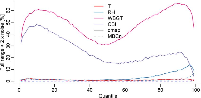
30 % and 70 % for WBGT (Fig. 9). If we use MBCn to ad- ties related to internal variability and the use of an incomplete
just biases, the uncertainty associated with internal variabil- bias adjustment can lead to substantial uncertainty in mul-
www.earth-syst-dynam.net/10/31/2019/ Earth Syst. Dynam., 10, 31–43, 201938 J. Zscheischler et al.: The effect of univariate bias adjustment on multivariate hazard estimates
Figure 8. (a) Ratio between full range and noise (uncertainty associated with internal variability) at the 90th percentile of heat stress (WBGT)
based on a perfect model approach using UQM to adjust biases; (b) ratio between the range of all models and the range of all five CanESM
runs of correlation between temperature and relative humidity.
duces biases in the indicator without the need to consider the
dependence between the drivers. Similarly, Casanueva et al.
(2018) studied the implications of component-wise bias ad-
justment on fire risk in Spain and find that there is little differ-
ence between separately adjusting the drivers before comput-
ing the hazard indicator and adjusting the hazard estimate di-
rectly. Räty et al. (2018) conclude, for hydrological variables,
that for most impacts, univariate methods have a compara-
ble performance to bivariate methods. In contrast, Cannon
(2018) clearly shows that including the dependence struc-
ture of drivers into the bias-adjustment procedure strongly
Figure 9. Fraction of grid points for which the full range is at reduces biases in the Canadian Fire Weather Index. Thus, we
least twice the range of the noise (uncertainty associated with inter- cannot draw the general conclusion that multivariate bias ad-
nal variability) in the perfect model approach. Solid lines represent justment is not necessary in any case from individual, typ-
cases computed with UQM; dashed lines represent cases computed ically regional, studies. Our findings suggest that whether
with MBCn.
bias-adjustment approaches lead to a substantial improve-
ment of impact indicators ultimately depends on (i) how large
the initial model biases are, (ii) how strongly the indicator
tivariate hazards, particularly for more extreme percentiles. truly depends on multiple variables, and (iii) how well the
The large increase in uncertainty illustrated by the full range models simulate relevant dependencies between the climate
stems from a combination of initial uncertainty related to in- variables (Fig. 6). Overall, it is difficult to pin down under
ternal variability and the inability of UQM to adjust depen- which exact circumstances univariate bias adjustment might
dencies adequately. Therefore, uncertainties related to inter- fail. We assume that modeled impacts that truly depend on
nal variability or other types of uncertainties may be strongly multiple dependent climate drivers are particularly suscepti-
increased by incomplete bias adjustment. These uncertain- ble to these issues. Impacts that fall into that category include
ties are likely sensitive to the length of the time period, as heat-related mortality (mostly depending on temperature and
longer time periods will reduce the noise component related humidity but also other factors), agricultural yields and car-
to internal variability due to a better sampling of the tails. bon uptake (temperature, precipitation, radiation), drought
These types of uncertainty are typically not communicated (precipitation, evapotranspiration), and the security of en-
and accounted for in impact modeling chains. Hence, to be ergy supply in a system that combines input from various re-
fully transparent, impact modeling should account for uncer- newable energy sources (radiation, precipitation, wind speed;
tainties associated with the chosen bias-adjustment approach Sterl et al., 2018). Impacts that might be less affected by
in addition to uncertainties related to the choice of climate these issues are those that predominantly depend on a sin-
model and impact model. gle climate variable such as runoff or floods, which mostly
Our results challenge the general applicability of conclu- rely on precipitation (Räty et al., 2018). In these cases, the
sions from previous studies that have investigated whether adjustment of the spatial and temporal distribution of precip-
a bias adjustment that is separately applied to all compo- itation might by more relevant than the adjustment of depen-
nents of a hazard indicator can effectively reduce biases in dencies between precipitation and other climate variables. A
the latter. For instance, Yang et al. (2015) studied the effect bias-adjustment method that is able to deal with very high di-
of component-wise bias adjustment on a fire risk indicator mensionality, for instance occurring when adjusting the co-
in Sweden and conclude that bias adjusting more drivers re-
Earth Syst. Dynam., 10, 31–43, 2019 www.earth-syst-dynam.net/10/31/2019/J. Zscheischler et al.: The effect of univariate bias adjustment on multivariate hazard estimates 39
variance between many locations at the same time, was re- 5 Conclusions
cently proposed by Vrac (2018).
While efforts to improve climate models and reduce their Climate impact modeling is crucial to translate informa-
biases will continue (Wang et al., 2014; Davin et al., 2016; tion from climate projections into potential impacts to aid
Kay et al., 2016), impact assessments need to become decision-making and planning. Due to persistent biases in
more transparent. In particular, uncertainties need to be well current climate models, bias adjustment is an integral part
communicated to aid adaptation planning (Wilby and Des- of most impact modeling activities. Our results demonstrate
sai, 2010). Many artifacts of currently widely used bias- that univariate bias adjustment can increase biases of sim-
adjustment methods are probably unknown because of the ulated hazards that depend on multiple correlated climatic
way bias adjustment is evaluated (Addor and Fischer, 2015; drivers. Univariate bias adjustment can furthermore lead to
Maraun et al., 2017). Evaluation of multivariate relation- a large increase in the uncertainty of such modeled hazards
ships and extremes need to become standard in the evalua- and impacts. Both aspects are particularly severe when study-
tion of climate and impact models as well as an evaluation of ing extremes. More importantly, if univariate bias adjustment
the appropriateness of the chosen bias-adjustment approach does not adequately adjust biases in hazards in the present-
(Cortés-Hernández et al., 2016; Zscheischler et al., 2018). day climate, future projections of such hazards have to be
Overall, multivariate bias-adjustment methods should be fa- interpreted very carefully. Our findings highlight that impact
vored in impact modeling to ensure that multivariate impacts modeling chains need to incorporate uncertainties associated
are captured more realistically. with the choice of bias adjustment into their uncertainty as-
As long as major biases in climate models persist, some sessment to be transparent for decision makers.
form of bias adjustment is unavoidable in model climate
impacts. In the fortunate case where large multimodel en-
sembles are available and a clear target is identified, ensem- Code and data availability. All datasets and the code to compute
ble members can be selected according to how well they the different bias adjustments are freely available from the sources
mentioned in Sect. 2 (Data and methods).
match certain criteria associated with the target (Sippel et al.,
2016; Maraun et al., 2017; Herger et al., 2018). Process-
based observational constraints (Hall and Qu, 2006; Sippel
et al., 2017; Vogel et al., 2018) are one way forward to se-
lect the most promising subset of models (Maraun et al.,
2017). Yet, in many cases, this information is not available
and large model ensembles may be too expensive to obtain.
To achieve the most reliable outcome with respect to mod-
eled impacts, bias adjustment preferably takes into account
the known limitations of the relevant climate model as well
as characteristics of the target system for which the bias ad-
justment is applied (Maraun et al., 2017). In large-scale im-
pact modeling projects such as ISIMIP, global flood model-
ing (Winsemius et al., 2015), global crop modeling (Ruane
et al., 2017), and generic modeling of high-impact events
(Done et al., 2015), achieving these standards is extremely
challenging, if not unfeasible. In these cases, typically, a sin-
gle bias-adjustment method is applied to a set of climate vari-
ables that then serves as input for a variety of impact models
across regions and sectors. The usefulness of such one-size-
fits-all approaches may be debated (Maraun et al., 2017), yet
decision makers urgently require robust information on po-
tential impacts of climate change. Impact modeling frame-
works such as ISIMIP and many others sample the uncer-
tainty related to the chosen climate model and impact model
but do not take into account uncertainties related to the ap-
plied bias-adjustment method. To be transparent towards po-
tential users, however, the scientific community should pro-
vide information on all uncertainties associated with mod-
eled impacts.
www.earth-syst-dynam.net/10/31/2019/ Earth Syst. Dynam., 10, 31–43, 201940 J. Zscheischler et al.: The effect of univariate bias adjustment on multivariate hazard estimates
Appendix A
Table A1. The 29 CMIP5 models used in this study. We use daily data from the historical simulation during the period 1981–1995.
Model name Modeling center Initialization
ACCESS1.0 Commonwealth Scientific and Industrial Research Organisation (CSIRO) and Bureau r1i1p1
of Meteorology (BOM), Australia
ACCESS1.3 Commonwealth Scientific and Industrial Research Organisation (CSIRO) and Bureau r1i1p1
of Meteorology (BOM), Australia
BCC-CSM1.1 Beijing Climate Center, China Meteorological Administration r1i1p1
BCC-CSM1.1M Beijing Climate Center, China Meteorological Administration r1i1p1
CanESM2 Canadian Centre for Climate Modelling and Analysis r1i1p1–r1i1p5
CNRM-CM5 Centre National de Recherches Météorologiques / Centre Européen de Recherche et r1i1p1
Formation Avancée en Calcul Scientifique
CSIRO-Mk3.6.0 Commonwealth Scientific and Industrial Research Organisation in collaboration with r1i1p1
Queensland Climate Change Centre of Excellence
GFDL-CM3 NOAA Geophysical Fluid Dynamics Laboratory r1i1p1
GFDL-ESM2G NOAA Geophysical Fluid Dynamics Laboratory r1i1p1
GFDL-ESM2M NOAA Geophysical Fluid Dynamics Laboratory r1i1p1
INM-CM4 Institute for Numerical Mathematics r1i1p1
IPSL-CM5A-LR Institut Pierre-Simon Laplace r1i1p1–r1i1p4
IPSL-CM5A-MR Institut Pierre-Simon Laplace r1i1p1
IPSL-CM5B-LR Institut Pierre-Simon Laplace r1i1p1
MIROC-ESM Japan Agency for Marine-Earth Science and Technology, Atmosphere and Ocean Re- r1i1p1
search Institute (The University of Tokyo), and National Institute for Environmental
Studies
MIROC-ESM-CHEM Japan Agency for Marine-Earth Science and Technology, Atmosphere and Ocean Re- r1i1p1
search Institute (The University of Tokyo), and National Institute for Environmental
Studies
MIROC5 Atmosphere and Ocean Research Institute (The University of Tokyo), National Institute r1i1p1–r1i1p3
for Environmental Studies, and Japan Agency for Marine-Earth Science and Technol-
ogy
MRI-CGCM3 Meteorological Research Institute r1i1p1
MRI-ESM1 Meteorological Research Institute r1i1p1
NorESM1-M Norwegian Climate Centre r1i1p1
Earth Syst. Dynam., 10, 31–43, 2019 www.earth-syst-dynam.net/10/31/2019/J. Zscheischler et al.: The effect of univariate bias adjustment on multivariate hazard estimates 41
Author contributions. JZ and EMF conceived the study. SL com- ment function diagnostic tool, Climatic Change, 147, 411–425,
puted the bias adjustment following the ISIMIP2b scheme. JZ ana- https://doi.org/10.1007/s10584-018-2167-5, 2018.
lyzed all data and produced all figures. JZ wrote the first draft, all Chandler, C., Cheney, P., Thomas, P., Trabaud, L., and Williams,
authors commented on the draft and all revisions. D.: Fire in forestry. Volume 1. Forest fire behavior and effects.,
John Wiley & Sons, Inc., New York, USA, 1983.
Chen, C., Haerter, J. O., Hagemann, S., and Piani, C.: On the con-
Competing interests. The authors declare that they have no con- tribution of statistical bias correction to the uncertainty in the
flict of interest. projected hydrological cycle, Geophys. Res. Lett., 38, L20 403,
https://doi.org/10.1029/2011GL049318, 2011.
Christensen, J. H., Boberg, F., Christensen, O. B., and Lucas-
Acknowledgements. We thank Alex Cannon for helpful dis- Picher, P.: On the need for bias correction of regional climate
cussions related to the application of the MBCn approach. Jakob change projections of temperature and precipitation, Geophys.
Zscheischler acknowledges financial support from the SNSF Res. Lett., 35, L20709, https://doi.org/10.1029/2008GL035694,
(Ambizione grant PZ00P2_179876). Stefan Lange acknowledges 2008.
funding from the European Union’s Horizon 2020 research Cortés-Hernández, V. E., Zheng, F., Evans, J., Lambert, M., Sharma,
and innovation program under grant agreement no. 641816 A., and Westra, S.: Evaluating regional climate models for simu-
(CRESCENDO). lating sub-daily rainfall extremes, Clim. Dynam., 47, 1613–1628,
https://doi.org/10.1007/s00382-015-2923-4, 2016.
Edited by: Ben Kravitz Cramer, W., Yohe, G. W., Auffhammer, M., Huggel, C., Molau, U.,
Reviewed by: Stefan Hagemann and one anonymous referee Dias, M. A. F. S., Solow, A., Stone, D. A., and Tibig, L.: De-
tection and attribution of observed impacts, in: Climate Change
2014: Impacts, Adaptation, and Vulnerability. Part A: Global and
Sectoral Aspects. Contribution of Working Group II to the Fifth
Assessment Report of the Intergovernmental Panel of Climate
References Change, edited by: Field, C. B., Barros, V. R., Dokken, D. J.,
Mach, K. J., Mastrandrea, M. D., Bilir, T. E., Chatterjee, M., Ebi,
Addor, N. and Fischer, E. M.: The influence of natural vari- K. L., Estrada, Y. O., Genova, R. C., Girma, B., Kissel, E. S.,
ability and interpolation errors on bias characterization in Levy, A. N., MacCracken, S., Mastrandrea, P. R., and White,
RCM simulations, J. Geophys. Res.-Atmos., 120, 10180–10195, L. L., 979–1037, Cambridge University Press, Cambridge, UK
https://doi.org/10.1002/2014JD022824, 2015. and New York, NY, USA, 2014.
Bosshard, T., Carambia, M., Goergen, K., Kotlarski, S., Davin, E. L., Maisonnave, E., and Seneviratne, S. I.: Is land sur-
Krahe, P., Zappa, M., and Schär, C.: Quantifying uncer- face processes representation a possible weak link in current
tainty sources in an ensemble of hydrological climate- Regional Climate Models?, Environ. Res. Lett., 11, 074027,
impact projections, Water Resour. Res., 49, 1523–1536, https://doi.org/10.1088/1748-9326/11/7/074027, 2016.
https://doi.org/10.1029/2011WR011533, 2013. Dee, D., Uppala, S., Simmons, A., Berrisford, P., Poli, P.,
Brando, P. M., Balch, J. K., Nepstad, D. C., Morton, D. C., Putz, Kobayashi, S., Andrae, U., Balmaseda, M., Balsamo, G., Bauer,
F. E., Coe, M. T., Silvério, D., Macedo, M. N., Davidson, E. A., P., Bechtold, P., Beljaars, A. C. M., van de Berg, L., Bidlot, J.,
Nóbrega, C. C., Alencar, A., and Soares-Filho, B. S.: Abrupt in- Bormann, N., Delsol, C., Dragani, R., Fuentes, M., Geer, A. J.,
creases in Amazonian tree mortality due to drought–fire interac- Haimberger, L., Healy, S. B., Hersbach, H., Hólm, E. V., Isak-
tions, P. Natl. Acad. Sci. USA, 111, 6347–6352, 2014. sen, L., Kållberg, P., Köhler, M., Matricardi, M., McNally, A. P.,
Bröde, P., Blazejczyk, K., Fiala, D., Havenith, G., Holmér, I., Jen- Monge-Sanz, B. M., Morcrette, J.-J., Park, B.-K., Peubey, C.,
dritzky, G., Kuklane, K., and Kampmann, B.: The Universal de Rosnay, P., Tavolato, C., Thépaut, J.-N., and Vitart, F.: The
Thermal Climate Index UTCI Compared to Ergonomics Stan- ERA-Interim reanalysis: Configuration and performance of the
dards for Assessing the Thermal Environment, Ind. Health, 51, data assimilation system, Q. J. Roy. Meteor. Soc., 137, 553–597,
16–24, https://doi.org/10.2486/indhealth.2012-0098, 2013. 2011.
Cannon, A. J.: Multivariate Bias Correction of Climate Model Done, J. M., Holland, G. J., Bruyère, C. L., Leung, L. R., and
Output: Matching Marginal Distributions and Intervari- Suzuki-Parker, A.: Modeling high-impact weather and climate:
able Dependence Structure, J. Climate, 29, 7045–7064, lessons from a tropical cyclone perspective, Clim. Change, 129,
https://doi.org/10.1175/jcli-d-15-0679.1, 2016. 381–395, https://doi.org/10.1007/s10584-013-0954-6, 2015.
Cannon, A. J.: Multivariate quantile mapping bias correction: an N- Dunne, J. P., Stouffer, R. J., and John, J. G.: Reductions in labour
dimensional probability density function transform for climate capacity from heat stress under climate warming, Nat. Clim.
model simulations of multiple variables, Clim. Dynam., 50, 31– Change., 3, 563–566, https://doi.org/10.1038/nclimate1827,
49, https://doi.org/10.1007/s00382-017-3580-6, 2018. 2013.
Carlson, J. D. and Burgan, R. E.: Review of users’ Ehret, U., Zehe, E., Wulfmeyer, V., Warrach-Sagi, K., and Liebert,
needs in operational fire danger estimation: The Ok- J.: HESS Opinions “Should we apply bias correction to global
lahoma example, Int. J. Remote Sens., 24, 1601–1620, and regional climate model data?”, Hydrol. Earth Syst. Sci., 16,
https://doi.org/10.1080/01431160210144651, 2003. 3391–3404, https://doi.org/10.5194/hess-16-3391-2012, 2012.
Casanueva, A., Bedia, J., Herrera, S., Fernández, J., and Elía, R. d., Laprise, R., and Denis, B.: Forecasting Skill Limits of
Gutiérrez, J. M.: Direct and component-wise bias correc- Nested, Limited-Area Models: A Perfect-Model Approach, Mon.
tion of multi-variate climate indices: the percentile adjust-
www.earth-syst-dynam.net/10/31/2019/ Earth Syst. Dynam., 10, 31–43, 201942 J. Zscheischler et al.: The effect of univariate bias adjustment on multivariate hazard estimates Weather Rev., 130, 2006–2023, https://doi.org/10.1175/1520- nity Earth System Model (CESM), J. Climate, 29, 4617–4636, 0493(2002)1302.0.co;2, 2002. https://doi.org/10.1175/jcli-d-15-0358.1, 2016. Fischer, E., Beyerle, U., and Knutti, R.: Robust spatially aggregated Kotlarski, S., Keuler, K., Christensen, O. B., Colette, A., Déqué, projections of climate extremes, Nat. Clim. Change, 3, 1033– M., Gobiet, A., Goergen, K., Jacob, D., Lüthi, D., van Meij- 1038, 2013. gaard, E., Nikulin, G., Schär, C., Teichmann, C., Vautard, R., Flato, G., Marotzke, J., Abiodun, B., Braconnot, P., Chou, S., Warrach-Sagi, K., and Wulfmeyer, V.: Regional climate model- Collins, W., Cox, P., Driouech, F., Emori, S., Eyring, V., For- ing on European scales: a joint standard evaluation of the EURO- est, C., Gleckler, P., Guilyardi, E., Jakob, C., Kattsov, V., Rea- CORDEX RCM ensemble, Geosci. Model Dev., 7, 1297–1333, son, C., and Rummukainen, M.: Evaluation of Climate Models, https://doi.org/10.5194/gmd-7-1297-2014, 2014. in: Climate Change 2013: The Physical Science Basis. Contribu- Lange, S.: EartH2Observe, WFDEI and ERA-Interim data tion of Working Group I to the Fifth Assessment Report of the Merged and Bias-corrected for ISIMIP (EWEMBI), Intergovernmental Panel on Climate Change, edited by: Stocker, https://doi.org/10.5880/pik.2016.004, 2016. T., Qin, D., Plattner, G.-K., Tignor, M., Allen, S., Boschung, J., Lange, S.: ISIMIP2b Bias-Correction Code, Nauels, A., Xia, Y., Bex, V., and Midgley, P., 741–866, Cam- https://doi.org/10.5281/zenodo.1069050, 2017. bridge University Press, Cambridge, UK and New York, NY, Lange, S.: Bias correction of surface downwelling longwave and USA, https://doi.org/10.1017/CBO9781107415324.020, 2013. shortwave radiation for the EWEMBI dataset, Earth Syst. Dy- Frieler, K., Lange, S., Piontek, F., Reyer, C. P. O., Schewe, J., nam., 9, 627–645, https://doi.org/10.5194/esd-9-627-2018, 2018. Warszawski, L., Zhao, F., Chini, L., Denvil, S., Emanuel, K., Lee, D. H. K.: Seventy-five years of searching for a heat in- Geiger, T., Halladay, K., Hurtt, G., Mengel, M., Murakami, D., dex, Environ. Res., 22, 331–356, https://doi.org/10.1016/0013- Ostberg, S., Popp, A., Riva, R., Stevanovic, M., Suzuki, T., 9351(80)90146-2, 1980. Volkholz, J., Burke, E., Ciais, P., Ebi, K., Eddy, T. D., Elliott, J., Li, C., Sinha, E., Horton, D. E., Diffenbaugh, N. S., and Micha- Galbraith, E., Gosling, S. N., Hattermann, F., Hickler, T., Hinkel, lak, A. M.: Joint bias correction of temperature and precipita- J., Hof, C., Huber, V., Jägermeyr, J., Krysanova, V., Marcé, R., tion in climate model simulations, J. Geophys. Res.-Atmos., 119, Müller Schmied, H., Mouratiadou, I., Pierson, D., Tittensor, D. 13153–13162, https://doi.org/10.1002/2014JD022514, 2014. P., Vautard, R., van Vliet, M., Biber, M. F., Betts, R. A., Bodirsky, Li, C., Zhang, X., Zwiers, F., Fang, Y., and Michalak, A. M.: B. L., Deryng, D., Frolking, S., Jones, C. D., Lotze, H. K., Lotze- Recent Very Hot Summers in Northern Hemispheric Land Campen, H., Sahajpal, R., Thonicke, K., Tian, H., and Yamagata, Areas Measured by Wet Bulb Globe Temperature Will Be Y.: Assessing the impacts of 1.5 ◦ C global warming – simula- the Norm Within 20 Years, Earth’s Future, 5, 1203–1216, tion protocol of the Inter-Sectoral Impact Model Intercompar- https://doi.org/10.1002/2017EF000639, 2017. ison Project (ISIMIP2b), Geosci. Model Dev., 10, 4321–4345, Maraun, D.: Bias Correction, Quantile Mapping, and Downscal- https://doi.org/10.5194/gmd-10-4321-2017, 2017. ing: Revisiting the Inflation Issue, J. Climate, 26, 2137–2143, Griffies, S. M. and Bryan, K.: A predictability study of simulated https://doi.org/10.1175/jcli-d-12-00821.1, 2013. North Atlantic multidecadal variability, Clim. Dynam., 13, 459– Maraun, D. and Widmann, M.: Cross-validation of bias-corrected 487, https://doi.org/10.1007/s003820050177, 1997. climate simulations is misleading, Hydrol. Earth Syst. Sci., 22, Gudmundsson, L.: qmap: Statistical transformations for postpro- 4867–4873, https://doi.org/10.5194/hess-22-4867-2018, 2018. cessing climate model output, R package version 1.0-2, 2014. Maraun, D., Shepherd, T. G., Widmann, M., Zappa, G., Walton, D., Hall, A. and Qu, X.: Using the current seasonal cycle to constrain Gutierrez, J. M., Hagemann, S., Richter, I., Soares, P. M. M., snow albedo feedback in future climate change, Geophys. Res. Hall, A., and Mearns, L. O.: Towards process-informed bias cor- Lett., 33, L03502, https://doi.org/10.1029/2005GL025127, 2006. rection of climate change simulations, Nat. Clim. Change, 7, Hawkins, E., Robson, J., Sutton, R., Smith, D., and Keenlyside, N.: 764–773, https://doi.org/10.1038/nclimate3418, 2017. Evaluating the potential for statistical decadal predictions of sea Martius, O., Pfahl, S., and Chevalier, C.: A global quantification of surface temperatures with a perfect model approach, Clim. Dy- compound precipitation and wind extremes, Geophys. Res. Lett., nam., 37, 2495–2509, https://doi.org/10.1007/s00382-011-1023- 43, 7709–7717, 2016. 3, 2011. McMichael, A. J., Woodruff, R. E., and Hales, S.: Climate change Hempel, S., Frieler, K., Warszawski, L., Schewe, J., and Piontek, and human health: present and future risks, Lancet, 367, 859– F.: A trend-preserving bias correction – the ISI-MIP approach, 869, 2006. Earth Syst. Dynam., 4, 219–236, https://doi.org/10.5194/esd-4- Mehrotra, R. and Sharma, A.: A Multivariate Quantile-Matching 219-2013, 2013. Bias Correction Approach with Auto- and Cross-Dependence Herger, N., Abramowitz, G., Knutti, R., Angélil, O., Lehmann, K., across Multiple Time Scales: Implications for Downscaling, and Sanderson, B. M.: Selecting a climate model subset to opti- J. Climate, 29, 3519–3539, https://doi.org/10.1175/JCLI-D-15- mise key ensemble properties, Earth Syst. Dynam., 9, 135–151, 0356.1, 2016. https://doi.org/10.5194/esd-9-135-2018, 2018. Pal, J. S. and Eltahir, E. A. B.: Future temperature in Humphrey, V., Zscheischler, J., Ciais, P., Gudmundsson, L., Sitch, southwest Asia projected to exceed a threshold for S., and Seneviratne, S.: Sensitivity of atmospheric CO2 growth human adaptability, Nat. Clim. Change, 6, 197–200, rate to observed changes in terrestrial water storage, Nature, 560, https://doi.org/10.1038/nclimate2833, 2015. 628–631, https://doi.org/10.1038/s41586-018-0424-4, 2018. Panofsky, H. and Brier, G.: Some Applications of Statistics to Mete- Kay, J. E., Wall, C., Yettella, V., Medeiros, B., Hannay, C., orology, The Pennsylvania State University, University Park, PA, Caldwell, P., and Bitz, C.: Global Climate Impacts of Fixing 1968. the Southern Ocean Shortwave Radiation Bias in the Commu- Earth Syst. Dynam., 10, 31–43, 2019 www.earth-syst-dynam.net/10/31/2019/
J. Zscheischler et al.: The effect of univariate bias adjustment on multivariate hazard estimates                                             43

Papadimitriou, L. V., Koutroulis, A. G., Grillakis, M. G., and Tsanis,    Vogel, M. M., Zscheischler, J., and Seneviratne, S. I.: Varying
   I. K.: The effect of GCM biases on global runoff simulations of          soil moisture-atmosphere feedbacks explain divergent temper-
   a land surface model, Hydrol. Earth Syst. Sci., 21, 4379–4401,           ature extremes and precipitation projections in central Europe,
   https://doi.org/10.5194/hess-21-4379-2017, 2017.                         Earth Syst. Dynam., 9, 1107–1125, https://doi.org/10.5194/esd-
Piani, C. and Haerter, J. O.: Two dimensional bias correction of tem-       9-1107-2018, 2018.
   perature and precipitation copulas in climate models, Geophys.         Vorogushyn, S., Bates, P. D., de Bruijn, K., Castellarin, A.,
   Res. Lett., 39, l20401, https://doi.org/10.1029/2012GL053839,            Kreibich, H., Priest, S., Schröter, K., Bagli, S., Blöschl, G.,
   2012.                                                                    Domeneghetti, A., Gouldby, B., Klijn, F., Lammersen, R., Neal,
Piani, C., Haerter, J. O., and Coppola, E.: Statistical bias                J. C., Ridder, N., Terink, W., Viavattene, C., Viglione, A., Za-
   correction for daily precipitation in regional climate mod-              nardo, S., and Merz, B.: Evolutionary leap in large-scale flood
   els over Europe, Theor. Appl. Climatol., 99, 187–192,                    risk assessment needed, Wiley Interdisciplinary Reviews: Water,
   https://doi.org/10.1007/s00704-009-0134-9, 2010.                         5, e1266, https://doi.org/10.1002/wat2.1266, 2018.
Räty, O., Räisänen, J., Bosshard, T., and Donnelly, C.: Intercompar-      Vrac, M.: Multivariate bias adjustment of high-dimensional climate
   ison of Univariate and Joint Bias Correction Methods in Chang-           simulations: the Rank Resampling for Distributions and Depen-
   ing Climate From a Hydrological Perspective, Climate, 6, 33,             dences (R 2 D 2 ) bias correction, Hydrol. Earth Syst. Sci., 22,
   https://doi.org/10.3390/cli6020033, 2018.                                3175–3196, https://doi.org/10.5194/hess-22-3175-2018, 2018.
Ruane, A. C., Rosenzweig, C., Asseng, S., Boote, K. J., El-               Vrac, M. and Friederichs, P.: Multivariate-intervariable, spatial, and
   liott, J., Ewert, F., Jones, J. W., Martre, P., McDermid, S. P.,         temporal-bias correction, J. Climate, 28, 218–237, 2015.
   Müller, C., Snyder, A., and Thorburn, P. J.: An AgMIP                  Wang, C., Zhang, L., Lee, S.-K., Wu, L., and Mechoso, C. R.: A
   framework for improved agricultural representation in inte-              global perspective on CMIP5 climate model biases, Nat. Clim.
   grated assessment models, Environ. Res. Lett., 12, 125003,               Change, 4, 201–205, https://doi.org/10.1038/nclimate2118,
   https://doi.org/10.1088/1748-9326/aa8da6, 2017.                          2014.
Semenov, M. A. and Porter, J. R.: Climatic variability and the            Wilby, R. L. and Dessai, S.: Robust adaptation to climate change,
   modelling of crop yields, Agr. Forest Meteorol., 73, 265–283,            Weather, 65, 180–185, https://doi.org/10.1002/wea.543, 2010.
   https://doi.org/10.1016/0168-1923(94)05078-K, 1995.                    Winsemius, H. C., Aerts, J. J. H., van Beek, L. H., Bierkens,
Sippel, S., Otto, F. E. L., Forkel, M., Allen, M. R., Guillod, B.           M. P., Bouwman, A., Jongman, B., Kwadijk, J. J., Ligtvoet,
   P., Heimann, M., Reichstein, M., Seneviratne, S. I., Thonicke,           W., Lucas, P., vanVuuren, D., and Ward, P.: Global drivers
   K., and Mahecha, M. D.: A novel bias correction methodology              of future river flood risk, Nat. Clim. Change, 6, 381–385,
   for climate impact simulations, Earth Syst. Dynam., 7, 71–88,            https://doi.org/10.1038/nclimate2893, 2015.
   https://doi.org/10.5194/esd-7-71-2016, 2016.                           Yang, W., Gardelin, M., Olsson, J., and Bosshard, T.: Multi-variable
Sippel, S., Zscheischler, J., Mahecha, M. D., Orth, R., Reichstein,         bias correction: application of forest fire risk in present and future
   M., Vogel, M., and Seneviratne, S. I.: Refining multi-model pro-         climate in Sweden, Nat. Hazards Earth Syst. Sci., 15, 2037–2057,
   jections of temperature extremes by evaluation against land-             https://doi.org/10.5194/nhess-15-2037-2015, 2015.
   atmosphere coupling diagnostics, Earth Syst. Dynam., 8, 387–           Zhao, Y., Ducharne, A., Sultan, B., Braconnot, P., and Vau-
   403, https://doi.org/10.5194/esd-8-387-2017, 2017.                       tard, R.: Estimating heat stress from climate-based indicators:
Sterl, S., Liersch, S., Koch, H., van Lipzig, N. P. M., and Thiery, W.:     present-day biases and future spreads in the CMIP5 global
   A new approach for assessing synergies of solar and wind power:          climate model ensemble, Environ. Res. Lett., 10, 084013,
   implications for West Africa, Environ. Res. Lett., 13, 094009,           https://doi.org/10.1088/1748-9326/10/8/084013, 2015.
   https://doi.org/10.1088/1748-9326/aad8f6, 2018.                        Zscheischler, J. and Seneviratne, S. I.: Dependence of drivers af-
Switanek, M. B., Troch, P. A., Castro, C. L., Leuprecht, A., Chang,         fects risks associated with compound events, Science Advances,
   H.-I., Mukherjee, R., and Demaria, E. M. C.: Scaled distribution         3, e1700263, https://doi.org/10.1126/sciadv.1700263, 2017.
   mapping: a bias correction method that preserves raw climate           Zscheischler, J., Orth, R., and Seneviratne, S. I.: Bivariate return
   model projected changes, Hydrol. Earth Syst. Sci., 21, 2649–             periods of temperature and precipitation explain a large frac-
   2666, https://doi.org/10.5194/hess-21-2649-2017, 2017.                   tion of European crop yields, Biogeosciences, 14, 3309–3320,
Taylor, K. E., Stouffer, R. J., and Meehl, G. A.: An Overview of            https://doi.org/10.5194/bg-14-3309-2017, 2017.
   CMIP5 and the Experiment Design, B. Am. Meteorol. Soc., 93,            Zscheischler, J., Westra, S., van den Hurk, B. J. J., Pitman, A.,
   485–498, https://doi.org/10.1175/BAMS-D-11-00094.1, 2012.                Ward, P., Bresch, D. N., Leonard, M., Zhang, X., AghaK-
Teutschbein, C. and Seibert, J.: Bias correction of regional climate        ouchak, A., Wahl, T., and Seneviratne, S. I.: Future climate
   model simulations for hydrological climate-change impact stud-           risk from compound events, Nat. Clim. Change, 8, 469–477,
   ies: Review and evaluation of different methods, J. Hydrol., 456–        https://doi.org/10.1038/s41558-018-0156-3, 2018.
   457, 12–29, 2012.
Van Loon, A. F., Gleeson, T., Clark, J., Van Dijk, A. I. J. M., Stahl,
   K., Hannaford, J., Di Baldassarre, G., Teuling, A. J., Tallaksen,
   L. M., Uijlenhoet, R., Hannah, D. M., Sheffield, J., Svoboda,
   M., Verbeiren, B., Wagener, T., Rangecroft, S., Wanders, N., and
   Van Lanen, H. A. J.: Drought in the Anthropocene, Nat. Geosci.,
   9, 89–91, https://doi.org/10.1038/ngeo2646, 2016.

www.earth-syst-dynam.net/10/31/2019/                                                               Earth Syst. Dynam., 10, 31–43, 2019
You can also read