Potential yield simulated by global gridded crop models: using a process-based emulator to explain their differences - GMD
←
→
Page content transcription
If your browser does not render page correctly, please read the page content below
Geosci. Model Dev., 14, 1639–1656, 2021
https://doi.org/10.5194/gmd-14-1639-2021
© Author(s) 2021. This work is distributed under
the Creative Commons Attribution 4.0 License.

Potential yield simulated by global gridded crop models: using a
process-based emulator to explain their differences
Bruno Ringeval1 , Christoph Müller2 , Thomas A. M. Pugh3 , Nathaniel D. Mueller4 , Philippe Ciais5 ,
Christian Folberth6 , Wenfeng Liu7 , Philippe Debaeke8 , and Sylvain Pellerin1
1 ISPA, Bordeaux Sciences Agro, INRAE, 33140, Villenave d’Ornon, France
2 Potsdam  Institute for Climate Impact Research, Member of the Leibniz Association, Potsdam, Germany
3 School of Geography, Earth & Environmental Science and Birmingham Institute of Forest Research,

University of Birmingham, Birmingham, UK
4 Department of Earth System Science, University of California, Irvine, CA, USA
5 Laboratoire de Sciences du Climat et de l’Environnement, LSCE/IPSL, CEA-CNRS-UVSQ,

Université Paris-Saclay, 91191, Gif-sur-Yvette, France
6 Ecosystem Services and Management Program, International Institute for Applied Systems Analysis,

2361 Laxenburg, Austria
7 College of Water Resources and Civil Engineering, China Agricultural University, Beijing 100083, China
8 AGIR, University of Toulouse, INRAE, 31326, Castanet-Tolosan, France

Correspondence: Bruno Ringeval (bruno.ringeval@inrae.fr)

Received: 17 April 2020 – Discussion started: 24 June 2020
Revised: 6 January 2021 – Accepted: 12 February 2021 – Published: 23 March 2021

Abstract. How global gridded crop models (GGCMs) differ         form RUE, then the simple set of equations of the SMM em-
in their simulation of potential yield and reasons for those    ulator is sufficient to reproduce the spatial distribution of the
differences have never been assessed. The GGCM Intercom-        original aboveground biomass simulated by most GGCMs.
parison (GGCMI) offers a good framework for this assess-        The grain filling is simulated in SMM by considering a fixed-
ment. Here, we built an emulator (called SMM for simple         in-time fraction of net primary productivity allocated to the
mechanistic model) of GGCMs based on generic and sim-           grains (frac) once a threshold in leaves number (nthresh ) is
plified formalism. The SMM equations describe crop phe-         reached. Once calibrated, these two parameters allow for the
nology by a sum of growing degree days, canopy radiation        capture of the relationship between potential yield and final
absorption by the Beer–Lambert law, and its conversion into     aboveground biomass of each GGCM. It is particularly im-
aboveground biomass by a radiation use efficiency (RUE).        portant as the divergence among GGCMs is larger for yield
We fitted the parameters of this emulator against gridded       than for aboveground biomass. Thus, we showed that the di-
aboveground maize biomass at the end of the growing sea-        vergence between GGCMs can be summarized by the differ-
son simulated by eight different GGCMs in a given year          ences in a few parameters. Our simple but mechanistic model
(2000). Our assumption is that the simple set of equations      could also be an interesting tool to test new developments
of SMM, after calibration, could reproduce the response of      in order to improve the simulation of potential yield at the
most GGCMs so that differences between GGCMs can be             global scale.
attributed to the parameters related to processes captured by
the emulator. Despite huge differences between GGCMs, we
show that if we fit both a parameter describing the thermal
requirement for leaf emergence by adjusting its value to each
grid-point in space, as done by GGCM modellers following
the GGCMI protocol, and a GGCM-dependent globally uni-

Published by Copernicus Publications on behalf of the European Geosciences Union.
1640                                                B. Ringeval et al.: Potential yield simulated by global gridded crop models

1   Introduction                                                       questions mentioned above. To do so, we first need to un-
                                                                       derstand how and why GGCMs potentially diverge in poten-
Potential yield corresponds to the yield achieved when an              tial yield simulation. The GGCM Intercomparison (GGCMI
adapted crop cultivar grows in non-limiting environmental              phase I) provides a framework relevant to the investigation
conditions (i.e., without water and nutrient stresses and in the       of the differences between GGCMs, as all GGCM modellers
absence of damages from weeds, pests, and diseases) under              followed the same protocol (Elliott et al., 2015). Model out-
a given crop management (e.g., plant density). Fundamen-               puts are available on the GGCMI data archive (Müller et al.,
tally, it is determined by a reduced number of environmental           2019). In the GGCMI framework, a simulation performed
variables: prevailing radiation, temperature, and atmospheric          with a harmonized growing period, absence of nutrient stress,
CO2 concentration. Biotic variables such as cultivar charac-           and irrigated conditions (see below) is particularly adapted
teristics (e.g., maturity group, leaf area index, root depth, har-     to simulate potential yield. Figure 1 displays the average
vest index), plant density and sowing date modulate how the            and coefficient of variation (CV) of such simulated above-
environmental conditions are converted into yield. At the lo-          ground biomass (biom) and yield (grain) for maize among
cal scale (field, farm, or small region), potential yields can         eight GGCMs participating in GGCMI that have been used
be estimated from field experiments, yield census, or crop             in our following analysis. While the GGCM divergence un-
growth models (Lobell et al., 2009). Crop simulation mod-              der potential conditions is lower than the GGCM divergence
els provide a robust approach because they account for the             when limiting factors are represented (Fig. S2 in the Supple-
interactive effects of genotype, weather, and management               ment), it remains relatively high. Figure 1 shows that the CV
(van Ittersum et al., 2013). These models are mathemati-               in potential conditions is higher for grain than for biom and
cal representations of our current understanding of biophys-           that the CV for grain can locally reach more than 50 %. To
ical crop processes (phenology, carbon assimilation, assimi-           understand what could explain these differences, we built a
late allocation) and of crop responses to environmental fac-           mechanistic emulator of GGCMs based on generic processes
tors. Such models have been designed to separate genotype–             controlling the accumulation of biomass (phenology from
environment–management interactions, for example via fac-              the sum of growing degree days, light absorption, radiation
torial simulations where one driver is varied at a time. Mod-          use efficiency) and the transformation of biomass into grain
els require site-specific inputs, such as daily weather data,          yield (trigger of yield formation, allocation of net primary
crop management practices (sowing date, cultivar maturity              production, NPP, to yield). We then calibrated the parame-
group, plant density, fertilization, and irrigation amounts and        ters of the emulator independently for each GGCM against
dates), and soil characteristics, with some of them being not          GGCM-simulated biom and the GGCM-simulated relation-
useful for the purpose of simulating potential yield. At the           ship between biom and grain. Our assumption is that a sim-
local scale, crop models can be calibrated to account for lo-          ple set of equations, with calibrated parameters, can repro-
cal specificities, in particular for specificities related to the      duce the outputs of most GGCMs and could be used to ex-
cultivar used at these sites (Grassini et al., 2011)                   plore the sources of differences between them. We choose
   Potential yield is also a variable of interest at large (coun-      to use a process-based (if very simple) model, as we expect
try, global) spatial scales, in particular as it is required for       that this model could propose interesting perspectives as ex-
yield gap analyses (van Ittersum et al., 2013; Lobell et al.,          plained in Sect. 4. In particular, if able to reproduce the re-
2009). Such analyses are necessary to get a large-scale pic-           sults of an ensemble of GGCMs, it could be an alternative
ture of yield limitations and to investigate questions related to      to the model ensemble mean or median usually used in in-
production improvement strategies, food security, and man-             tercomparison exercises (Martre et al., 2015). Running much
agement of resources with a global perspective. However,               faster than GGCMs, it would also be an interesting tool to
while crop models used at local scale can be calibrated to             test new developments, such as the implementation of culti-
account for local specificities, it is much more complicated           var diversity, to improve the simulation of potential yield at
to model the spatial variations of yields at the global scale.         the global scale.
Local crop models have been applied at the global scale ei-
ther directly or through the implementation of some of their
equations into global vegetation models (Elliott et al., 2015).        2     Methods
Global Gridded Crop Models (GGCMs in the following) pro-
vide spatially explicit outputs, typically at half-degree reso-        2.1    GGCM emulator
lution in latitude and longitude. Their simulations are prone
to uncertainty. In particular, it is quite difficult to get reliable   For any given day d of the growing season (defined here as
information about the diversity of cultivars (Folberth et al.,         the period between the planting day, tp , and the crop maturity,
2019) or crop management at the global scale with large ef-            tm ), we used the Eqs. (1)–(7), which rely on concepts com-
fects on the crop behavior (Drewniak et al., 2013).                    monly used in modeling of ecosystem productivity to com-
   Increasing our confidence in potential yield simulated by           pute the potential aboveground biomass (biom, in t DM ha−1 ,
GGCMs is required to improve our ability to reply to societal          with 1 ha = 0.01 km2 ). Variables and parameters are summa-

Geosci. Model Dev., 14, 1639–1656, 2021                                                https://doi.org/10.5194/gmd-14-1639-2021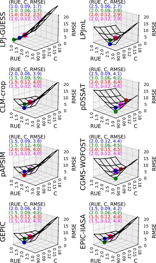
B. Ringeval et al.: Potential yield simulated by global gridded crop models                                                       1641

Figure 1. GGCM divergence in simulation of potential aboveground biomass and yield. Average and coefficient of variation for both above-
ground biomass (biom) and yield (grain) computed among eight GGCMs used in the current analysis for simulations approaching poten-
tial yield in GGCMI (i.e., harmnon × irrigated for LPJ-GUESS, LPJmL, CLM-crop, pDSSAT, pAPSIM, GEPIC, and EPIC-IIASA and
default × irrigated for CGMS-WOFOST; see Sect. 2.2.1). Only grid cells common to the eight GGCMs are considered for this figure. For
GEPIC and EPIC-IIASA, the variable biom has been corrected (see Sect. 2.2.1). For the comparison including GGCMs that provide biom and
grain for harmnon × irrigated simulation in GGCMI but which are not part of the current paper (i.e., EPIC-BOKU, PEPIC, and PEGASUS),
see Fig. S1 in the Supplement.

rized in Table 1, and a simplified flow chart is given in Fig. S3     is computed from APAR with a constant radiation use effi-
in the Supplement.                                                    ciency (RUE in g DM MJ−1 ):
   For any d in [tp , tm ], the thermal time (TT) is computed
from the daily mean temperature (tas, in ◦ C) by using a ref-         NPPbiom (d) = RUE × APAR (d) .                                (6)
erence temperature (T0 ):
                                                                         The aboveground biomass corresponds to the sum over
TT (d) = tas (d) − T0 .                                       (1)     time of NPPbiom :
                                                                                 X
GDD is the sum of growing degree days, defined as follows:            biom (d) =        (NPPbiom (i)) .                  (7)
                                                                                    i≤d
           X
GDD (d) =     i≤d
                  max (0, T T (i)) .                   (2)              The parameter C of Eq. (5) can be decomposed in different
                                                                      parameters:
The number of leaves per plant (nleaf ) is computed from
GDD and one parameter representing the thermal require-               C = k × Sleaf × dplant ,                                      (8)
ment for the emergence of any leaf (GDD1leaf ):
                                                                      where k is the light extinction coefficient, Sleaf is the individ-
nleaf (d) = min (maxnleaf , GDD (d) /GDD1leaf ) ,             (3)
                                                                      ual leaf area, and dplant is the plant density. The product of
where maxnleaf is the maximum number of leaves. In our                Sleaf , dplant and the number of leaves of a given day d (i.e.,
model, as soon as one leaf emerges, we assumed that it                nleaf (d)), corresponds to the leaf area index (LAI) of the same
reaches its fully expanded leaf area, which is the same for           day:
all leaves (individual leaf area, called Sleaf hereafter). The
                                                                      LAI (d) = Sleaf × dplant × nleaf (d) ,                        (9)
incoming photosynthetic active radiation (PARinc ) is de-
rived from the short-wave downwelling radiation (rsds in
                                                                      in such a way that Eq. (5) can be re-written as follows:
MJ m−2 d−1 ) and its active fraction, f :

PARinc (d) = f × rsds (d) .                                   (4)     APAR (d) = PARinc (d) × (1 − exp (−k × LAI (d))) (5bis),

  The absorbed PAR by the canopy (APAR) is determined                 We preferred Eq. (5) over Eq. (5bis) as we cannot separately
by assuming an exponential function according to the Beer–            calibrate the different parameters composing C and because
Lambert law:                                                          we do not have any information about the LAI from GGCMs
                                                                      (see Sect. 4).
APAR (d) = PARinc (d) × (1 − exp (−C × nleaf (d))) ,          (5)        To compute the grain biomass at maturity, we first define
                                                                      the day l as follows:
where C is a constant (see below). The net primary pro-
ductivity dedicated to the aboveground biomass (NPPbiom )             nleaf (l) ≥ nthresh ,                                        (10)

https://doi.org/10.5194/gmd-14-1639-2021                                                      Geosci. Model Dev., 14, 1639–1656, 2021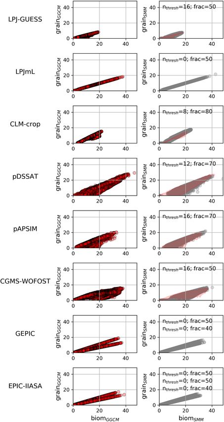
1642                                                    B. Ringeval et al.: Potential yield simulated by global gridded crop models

Table 1. List of variables and parameters in SMM.

                Definition                                     Unit                                Status
  tas           Daily mean temperature                         ◦C                                  Input variable
  TT            Thermal time                                   ◦C                                  Internal variable
  GDD           Sum of growing degree days                     ◦C                                  Internal variable
  nleaf         Number of leaves per plant                     –                                   Internal variable
  rsds          Short-wave downward radiation                  MJ m−2 d−1                          Input variable
  PARinc        Incoming photosynthetic active radia-          MJ m−2 d−1                          Internal variable
                tion
  APAR          Canopy-absorbed incoming PAR                   MJ m−2 d−1                          Internal variable
  NPPbiom       Net primary productivity dedicated to          g DM m−2 d−1                        Internal variable
                aboveground biomass
  biom          Aboveground biomass                            g DM m−2                            Internal variable. The study focuses on
                                                                                                   biom at the end of the growing sea-
                                                                                                   son, called biomSMM , and converted to
                                                                                                   t DM ha−1 .
  NPPgrain      Net primary productivity dedicated to          g DM m−2 d−1                        Internal variable
                grains
  grain         Grain biomass (yield)                          g DM m−2                            Internal variable. The study focuses on
                                                                                                   grain at the end of the growing sea-
                                                                                                   son, called grainSMM , and converted to
                                                                                                   t DM ha−1
  T0            Zero of vegetation                             ◦C                                  Parameter
  GDD1leaf      Sum of growing degree day required for         ◦C                                  Parameter
                each leaf (phyllochron)
  maxnleaf      Maximum number of leaves per plant             –                                   Parameter
  f             Active fraction of short-wave down-            –                                   Fixed parameter (f = 0.48)
                ward radiation
  C             C = k ×Sleaf ×dplant with k: coefficient       –                                   Parameter
                of extinction of radiation in canopy;
                Sleaf : the specific leaf area of any leaf
                and dplant : the plant density
  RUE           Radiation use efficiency                       g DM MJ−1 (Here, MJ refers to ab-   Parameter
                                                               sorbed PAR)
  nthresh       Number of leaves from which the for-           –                                   Parameter
                mation of reproductive structures starts,
                the grains form, or the grain filling starts
  frac          Fraction of NPPbiom going towards the          –                                   Parameter
                variable grain when nleaf > nthresh

From day l, a fixed fraction (frac) of NPPbiom constitutes                   the grains form, or grain filling starts. The above equations
the net primary productivity dedicated to the variable grain                 aim to be generic and to reproduce the diversity of ap-
(called NPPgrain ):                                                          proaches in GGCMs. That is why we do not distinguish be-
(                                                                            tween the production of reproductive structures and the ac-
  if d ≥ l, NPPgrain (d) = frac × NPPbiom (d) ,          (11)                cumulation of assimilates in grains after anthesis.
 if d < l,     NPPgrain (d) = 0.                                      (12)      Equations (1)–(7) and (10)–(13) are called SMM (for sim-
                                                                             ple mechanistic model) in the following. We focused on biom
and finally,                                                                 and grain at maturity, i.e., computed on the last day of the
               X                                                            growing season tm . They are called biomSMM and grainSMM
grain (d) =      i≤d
                       NPPgrain (i) .                               (13)

   The variable grain (in t DM ha−1 ) could be considered ei-
ther as reproductive structures + grains or grains only. The
parameter nthresh is a threshold in the number of leaves from
which either the formation of reproductive structures starts,

Geosci. Model Dev., 14, 1639–1656, 2021                                                      https://doi.org/10.5194/gmd-14-1639-2021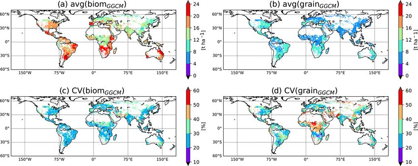
B. Ringeval et al.: Potential yield simulated by global gridded crop models                                                  1643

in the following:                                                 by the AgMERRA dataset as all GGCMs performed these
                                                                  simulations. Three levels of harmonization have been used
biomSMM = biom (tm ) ,                                    (14)    in GGCM simulations: default, fullharm, harmnon. In full-
grainSMM = grain (tm ) .                                  (15)    harm simulations, all GGCMs have been forced by the same
                                                                  prescribed beginning and end of the growing season, which
   The variable grainSMM is used to approach the potential        were derived from a combination of two global datasets
yield. Our analysis focuses on maize because of the impor-        (MIRCA, Portmann et al., 2010; and SAGE, Sacks et al.,
tance of cereals in human food and because of the widespread      2010; Elliott et al., 2015). In harmnon simulations, in ad-
distribution of this crop across latitudes.                       dition to forced timing and duration of the growing season,
                                                                  all GGCMs experienced no nutrient limitation through pre-
2.2     Set-up
                                                                  scribed fertilizer inputs. Besides this harmonization level,
We focused first on the computation of biomSMM and then           two water regimes have been considered: irrigated and non-
on the relationship grainSMM vs. biomSMM . The sensitiv-          irrigated. For our analysis focusing on the simulation of po-
ity of SMM to each parameter involved in the computa-             tential yield, we decided to select the configuration (harmnon
tion of biomSMM was first studied. Then, we calibrated            and irrigated). This is true for all GGCMs considered ex-
SMM against each GGCM to make the spatial distribution            cept CGMS-WOFOST. In fact, the harmnon simulation was
of biomSMM mimic the spatial distribution of aboveground          not provided for CGMS-WOFOST but because (i) this model
biomass at maturity simulated by each GGCM (hereafter             does not consider nutrient limitation and (ii) the growing sea-
called biomGGCM ). This calibration happened in two steps.        son was prescribed in the default simulation, we assumed that
The first step concerned C and RUE, which have one value          the potential yield could be approached by the (default and
at the global scale. The second step concerned GDD1leaf ,         irrigated) simulation.
which we made varying in space to mimic procedure used               For EPIC family models (here, GEPIC and EPIC-IIASA),
by GGCM modellers in GGCMI (see below). The choice of             we used a corrected biomGGCM computed as below, as it has
focusing on C, RUE, and GDD1leaf is justified below. In the       been noticed that some issues related to the variable biom ap-
last step (step 3), we calibrated nthresh and frac to make SMM    peared in the outputs available on the GGCMI data archive
mimic the relationship grain vs. biom of each GGCM.               that are likely related to the output time step of specific vari-
                                                                  ables (Folberth, personal communication, 2019):
2.2.1    GGCMs and GGCMI simulations considered
                                                                  biomGGCM = grainGGCM /HImax ,                               (16)
The eight GGCMs considered in our approach were LPJ-              where HImax is the maximum harvest index (no unit), vary-
GUESS (Lindeskog et al., 2013; Smith et al., 2001), LPJmL         ing in space as a function of cultivars. In EPIC, the actual
(Bondeau et al., 2007; Waha et al., 2012), CLM-crop (Drew-        HI at harvest only differs to HImax if a drought stress occurs
niak et al., 2013), pDSSAT (Elliott et al., 2014; Jones et al.,   in the reproductive phase. Because this stress was virtually
2003), pAPSIM (Elliott et al., 2014; Keating et al., 2003),       eliminated by sufficient irrigation in the harmnon × irrigated
CGMS-WOFOST (Boogaard et al., 2014), GEPIC (Williams              simulations, Eq. (16) provides the most accurate estimate of
et al., 1995; Folberth et al., 2012; Izaurralde et al., 2006;     aboveground biomass at harvest. Maps of cultivar distribu-
Liu et al., 2007), EPIC-IIASA (Williams et al., 1995; Iza-        tion, used as input to the EPIC models (Fig. 1 and Table D in
urralde et al., 2006). GGCMs simulations are provided in          Folberth et al., 2019), have been considered here to compute
the framework of the GGCM Intercomparison (GGCMI) and             the corrected biomGGCM .
described in Müller et al. (2019). GGCMI is an activity of
the of the Agricultural Model Intercomparison and Improve-        2.2.2   Input variables for SMM
ment Project (AgMIP; Rosenzweig et al., 2013) and is an el-
ement of a broader AgMIP effort to explore cropping system        We focused our analysis on the growing season starting in
responses to climate conditions and climate changes to fa-        calendar year 2000 (and potentially finishing in calendar year
cilitate applications including toward integrated assessment      2001). SMM was forced by the short-wave downwelling ra-
(Ruane et al., 2017). Six other GGCMs also participated           diation (rsds in MJ m−2 d−1 ) and the daily mean tempera-
in GGCMI but were not considered here as necessary out-           ture (tas, in ◦ C) from the AgMERRA weather dataset (Ru-
put variables (timing and duration of the growing season for      ane et al., 2015). SMM also needs the beginning and end of
EPIC-BOKU, PEPIC, EPIC-TAMU; aboveground biomass                  the maize growing season, and we used the planting day (tp )
for ORCHIDEE-crop) or simulations (for PRYSBI2) were              and the timing of maturity (tm ), respectively, both being pro-
not provided on the data archive of GGCMI.                        vided in the output of each GGCM. Despite the fact that all
   In GCCMI, all GGCMs followed a common protocol and             GGCMs are forced by the same growing season in harmnon,
were forced by the same weather datasets. We focused here         some GGCMs allow flexibility in regards to tp and tm pre-
on the simulations forced by one of them, the AgMERRA             scribed as input (Müller et al., 2017), as suggested by the
dataset (Ruane et al., 2015). We used simulations forced          GGCMI protocol: “crop variety parameters (e.g., required

https://doi.org/10.5194/gmd-14-1639-2021                                            Geosci. Model Dev., 14, 1639–1656, 2021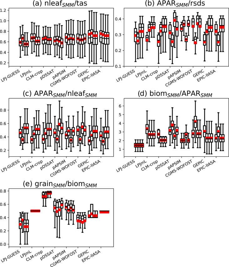
1644                                              B. Ringeval et al.: Potential yield simulated by global gridded crop models

growing degree days to reach maturity, vernalization require-       RUE000 = RUE0 /0.425) (Sinclair and Muchow, 1999), and
ments, photoperiodic sensitivity) should be adjusted as much        this could lead to erroneous values in GGCMs. In the follow-
as possible to roughly match reported maturity dates”. Thus,        ing we used MJ of absorbed PAR to be consistent with our
we cannot use tp and tm from GGCM input files (Text S1 in           Eq. (6). Observations also showed that RUE decreases during
the Supplement).                                                    grain filling following the mobilization of leaf nitrogen to the
   We performed SMM simulations (and thus, computed                 grain (Sinclair and Muchow, 1999). Thus, RUE is larger dur-
biomSMM and grainSMM ) for each GGCM, i.e., for each                ing vegetative growth (3.8–4.0 g DM (MJofabsorbedPAR)−1 ;
GGCM growing season. For a given GGCM, SMM simu-                    Kiniry et al., 1989) than averaged over the whole season
lations were performed only for grid cells considered in the        (3.1–4.0 g DM MJ−1 ; Sinclair and Muchow, 1999). It is likely
given GGCM. In addition, grid cells for which information           that some GGCMs used RUE values which are not represen-
about the growing season from MIRCA and SAGE was not                tative to the whole growing season. Thus, we used the same
available are masked to prevent to consider grid cells where        range of uncertainty for all parameters in our calibration pro-
internal GGCM computation was performed.                            cedure. Exploring a wider range of values also allows for a
   The maps of cultivar distribution used by EPIC models            more complete assessment of GGCM performance.
(Folberth et al., 2019) were also used as inputs to SMM in the         Potential confusion in units mentioned above also led
simulation aiming to mimic the biom vs. grain relationship of       us to choose an initial estimate of RUE (2 g DM MJ−1 )
EPIC models (see Sect. 2.2.4).                                      lower than values commonly reported in the literature (3.1–
                                                                    4.0 g DM MJ−1 ) (Sinclair and Muchow, 1999); however, note
2.2.3   Sensitivity of global biomSMM to SMM                        that the highest values of RUE tested during our calibration
        parameters                                                  (3.0 g DM MJ−1 ) reach the literature-based range.
                                                                       The global mismatch between each GGCM and SMM
Except the active fraction of short-wave downward radiation         was quantified thanks to the root-mean-square error (RMSE),
(f in Eq. 4) the value of which is physically well-known,           computed as follows:
other parameters involved in the computation of biomSMM
(T0 , maxnleaf , GDD1leaf , C, RUE) are relatively uncertain.       RMSE (u)                                         (17)
                                                                        r
The sensitivity of the global averaged biomSMM to these pa-               1  XN
rameters was assessed by performing 3125 (i.e., 55 ) SMM              =       g=1
                                                                                  (biomSMM (u, g) − biomGGCM (g))2 ,
                                                                          N
simulations, allowing for the combination of five different
values for each parameter. In each of these SMM simula-             where u is a combination of parameters and g is a grid cell
tions, a given parameter was constant in space. The initial         among the N grid cells considered for each GGCM. All grid
estimate of each parameter was provided in Table S1. While          cells are assumed independent and have the same weight in
the initial estimate of each parameter was based on the liter-      the RMSE computation. RMSE has the same unit as biom
ature, we chose quite arbitrarily the same range of variation       (t DM ha−1 ).
of [50 %–150 %] (in % of the initial estimate) for all param-
                                                                    2.2.4   SMM calibration against each GGCM
eters, with the five values tested uniformly distributed within
the range of variation (i.e., 50 %, 75 %, 100 %, 125 %, 150 %       SMM was calibrated following three steps. The first two
of initial guess).                                                  steps aimed to mimic biomGGCM distribution, while the last
   Following our current knowledge based on observations,           step aimed to make SMM reproduce the relationship grain vs.
it would be partly possible to choose a different uncertainty       biom of each GGCM. The procedure of calibration was sum-
range for each parameter: for instance, the literature tends        marized in Table 2. “Emulated GGCM” is used from now to
to show that RUE is relatively well constrained for maize           define SMM output after SMM calibration, aiming to mimic
(Sinclair and Muchow, 1999), while the C parameter, which           a given GGCM.
depends on plant density, is expected to vary a lot as a func-
tion of the farming practices (Sangoi et al., 2002; Testa et al.,   Parameters involved in the computation of biomSMM
2016) (Table S1). However, SMM aimed to mimic GGCMs
and not observations, and it is quite difficult to know if pa-      Regarding the simulation of biom, we restricted the cal-
rameter values used in GGCMs reflect our current knowl-             ibration to RUE, C, and GDD1leaf as follows: f is well
edge well. For instance, there is some confusion in values          constrained, maxnleaf has a small effect on global simu-
of RUE reported in the literature following the diversity of        lated biomSMM (see the results of the analysis prescribed
experimental approaches and units of expression that have           in Sect. 2.2.3), and T0 co-varies with GDD1leaf , and we de-
been used (Sinclair and Muchow, 1999). Some confusion in            cided to focus on GDD1leaf (see below). These parameters
RUE values exists in the literature between RUE expressed in        (f , maxnleaf , T0 ) were prescribed equal to their initial esti-
g DM MJ−1 of intercepted solar radiation (called here RUE0 )        mate and were the same for all SMM simulations.
or in g DM MJ−1 of intercepted PAR (RUE00 , with RUE00 =               We choose to make C and RUE globally constant and
RUE0 /0.5) or in g DM MJ−1 of absorbed PAR (RUE000 , with           GGCM-dependent. The decision to not make C and RUE

Geosci. Model Dev., 14, 1639–1656, 2021                                              https://doi.org/10.5194/gmd-14-1639-2021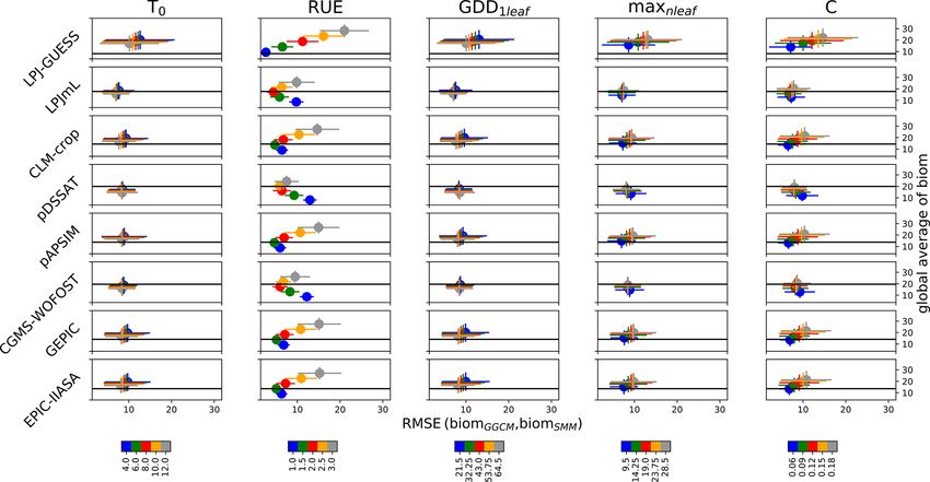
B. Ringeval et al.: Potential yield simulated by global gridded crop models 1645
Table 2. Strategy of SMM calibration for each parameter.
Step of calibration Parameters Values used in SMM simulations GGCM variable used for the calibration
f , T0 , maxnleaf One value at the global scale and same None
for all GGCMs
1 C, RUE One value at the global scale and Global averaged biom
GGCM-dependent
3 nthresh , frac∗ Relationship grain vs. biom
2 GDD1leaf Variable in space and GGCM- Spatial variability of biom
dependent variability
∗n
thresh and frac are variable in space as a function of the cultivar when SMM aims to mimic EPIC family models as these latter consider some cultivar diversity
in harvest index.
vary in space is consistent with the rule of parsimony, which temperatures and one sub-group with low temperatures) and
we used to build SMM. It also follows the procedure com- assess if the RMSE is different for the two sub-groups. If yes,
monly used in GGCMs that involved a similar approach. For it would suggest that a process related to this variable (e.g.,
instance, GEPIC is based on a biomass-energy conversion heat stress) could be missing in SMM.
coefficient that does not vary in space (Folberth et al., 2016).
Plant density (hidden in C) is constant in space in LPJmL Parameters involved in the computation of grainSMM
(Schaphoff et al., 2018a). We calibrated C and RUE at the
same time to assess potential compensation between these
C, RUE, and GDD1leaf determine biom simulated by SMM
parameters in SMM. The three pairs (C, RUE) that mini-
at each time step. Two SMM parameters are involved in the
mized the global RMSE computed following Eq. (17) the
computation of grain for any day from biom, namely nthresh
most among the pairs tested were chosen. A fourth pair corre-
and frac. The calibration of these parameters aims to make
sponding to (C, RUE), where C is equal to its initial estimate,
SMM able to mimic the relationship between grain and biom
has been used. The use of four different pairs aimed to assess
at the end of the growing season from each GGCM. One
the sensitivity of our conclusions to the parameter values. For
global and GGCM-dependent pair (nthresh , frac) was chosen
each (C, RUE) pair, we finally calibrated GDD1leaf . We made
by using the following criteria:
GDD1leaf vary in space as it is allowed in the GGCMI exer-
cise. In the GGCMI protocol, accumulated thermal require-
ments were adjusted to catch the growing season (duration if AGGCM = 0, find u that minimizes (19)
and timing) prescribed as input in the harmnon GGCM sim-
Rslope (u) = |aGGCM − aSMM (u)| ,
ulation. In SMM, the procedure slightly differs as we cali-
brated thermal requirements to match biomGGCM : for each
if AGGCM 6 = 0,find u that maximizes
(20)
AGGCM ∩ASMM (u)
grid cell, GDD1leaf is chosen among its five possible values R (u) = ,
areas max(AGGCM ,ASMM (u))
to minimize the absolute difference between biomGGCM and
biomSMM . Grid cells were considered independently.
The ability of SMM to match the spatial distribution of where u corresponds to a given pair (nthresh , frac), AX is the
biomGGCM for each GGCM after SMM calibration was mea- area defined by the grid cell clouds in the grain vs. biom
sured through the bias, RMSE, and Nash–Sutcliffe model ef- space for X, and aX is the slope of the linear regression
ficiency coefficient (NS), defined as follows: grainX ∼ biomX , with X in {GGCM, SMM}.
PN In other words, if grainGGCM vs. biomGGCM is a line,
2
g=1 (biomSMM (g) − biomGGCM (g)) (nthresh , frac) is chosen to make the relationship between
NS = 1 − P 2 , (18)
N grainSMM vs. biomSMM linear with the same slope as the
g=1 biomGGCM (g) − biomGGCM
one of the GGCM. If grainGGCM vs. biomGGCM is not a line,
where g refers to any grid cell and biomGGCM is the aver- the grid cells in the space grainGGCM vs. biomGGCM define a
age of biomGGCM over grid cells. NS = 1 means that SMM non-null area, called AGGCM , and (nthresh , frac) is chosen to
perfectly matches the spatial distribution of biomGGCM . make ASMM as similar as possible to AGGCM . EPIC family
To assess the mismatch between biomGGCM and biomSMM GGCMs introduced a cultivar diversity in parameters related
after SMM calibration for a given GGCM, we aimed to as- to grain filling and, in that case, the calibration of (nthresh ,
sess how a variable related to climate or soil type can con- frac), instead of being done at the global scale, was made for
tribute to this mismatch. To do so, we separated all grid cells each cluster of grid cells corresponding to a given cultivar.
within two sub-groups according to the value of this variable The distribution of cultivars from EPIC was used as input of
(e.g., one sub-group corresponding to grid cells with high SMM in that case.
https://doi.org/10.5194/gmd-14-1639-2021 Geosci. Model Dev., 14, 1639–1656, 20211646 B. Ringeval et al.: Potential yield simulated by global gridded crop models
2.3 Contribution of different processes to yield in SMM timate decreased the ability of SMM to match the GGCMs
only slightly (magenta dots in Fig. 3) and did not drastically
We computed ratios between some SMM internal variables change the RUE compared to the pairs where both C and
to assess the global contribution of different processes repre- RUE were calibrated.
sented in SMM to the achievement of grainSMM . The fol-
lowing ratios have been computed: nleaf /tas, APAR/rsds, 3.2 Calibration of GDD1leaf
APAR/nleaf , biom/APAR, and grain/biom. The ratio
nleaf /tas represents the phenology sensitivity to temperature, Once (C, RUE) was globally chosen, a spatially varying
APAR/rsds reflects how radiation is absorbed by the canopy, GDD1leaf was calibrated. After calibration, SMM was able to
APAR/nleaf represents the absorption sensitivity to phenol- catch the spatial variability of biomGGCM for most GGCMs
ogy, biom/APAR reflects the conversion from absorbed ra- (Figs. 4 and 5a). Difference in percent can be large, espe-
diation to biomass, and grain/biom represents the harvest in- cially for regions with small biom, but the global distribution
dex. was relatively well captured (Fig. 4).
We also investigated how the contribution of the differ- Global RMSE reaches between ∼ 1 (LPJ-GUESS) and
ent processes to the achievement of grainSMM varies between 3.3 t DM ha−1 (EPIC-IIASA) (Fig. 5a). The Nash–Sutcliffe
emulated GGCMs. Variations in these ratios reflects the dif- coefficient (NS) is large (≥ 0.6) for all GGCMs but CLM-
ference in global averaged key parameters between emulated crop (0.46) and pAPSIM (0.41). RMSE is greater if com-
GGCMs. For instance, variations in grain/biom between em- puted for grid cells that experience some days with tempera-
ulated GGCMs reflects differences in calibrated nthresh and ture above 30 ◦ C than if computed for grid cells without such
frac (Fig. S3). days, i.e., for LPJ-GUESS (1.5 t DM ha−1 vs. 0.8), GEPIC
To compute the different ratios, averages over the growing (4.4 vs. 2.3), EPIC-IIASA (4.2 vs. 2.8), and pAPSIM (3.5 vs.
season were used for tas, rsds, APAR, and nleaf , while the end 2.3) (not shown). Nevertheless, the implementation of a heat
of the growing season was used for biom and grain (so-called stress within SMM (Text S2 in the Supplement) only slightly
biomSMM and grainSMM , Eqs. 14 and 15). A given ratio was increases the fit of SMM vs. GGCM for these GGCMs: for
computed for each grid cell, and its grid-cell distribution was example, NS increases from 0.41 (without heat stress) to 0.52
plotted in the following as a bar plot (Sect. 3.4 and Fig. 8). (with heat stress) for pAPSIM (Fig. S5 in the Supplement).
The limited increase can be explained by the fact that opti-
mized GDD1leaf in the SMM simulation without heat stress
3 Results encompasses a part of the heat stress for these grid cells.
EPIC family GGCMs simulate some other stresses, such
3.1 Global averaged biomSMM : sensitivity to each as stresses related to salinity and aeration, that could have
parameter and calibration of (C, RUE) an effect on the potential yield even in the (harmnon and ir-
rigated) simulations (Müller et al., 2019). The intensity of
As expected when looking at Eqs. (6) and (7), the global av- some of these stresses (aeration) depends on soil orders and
eraged biomSMM sensitivity to RUE was large (Fig. 2). Vary- should be particularly important in Vertisols (Christian Fol-
ing RUE was the only way possible to capture the global berth, personal communication, 2019). However, RMSE is
averaged biomGGCM for LPJ-GUESS (Fig. 2). The global only slightly different for grid cells characterized by Verti-
averaged biomSMM was only slightly sensitive to other pa- sols vs. others soil orders for GEPIC (3.4 for Vertisols vs.
rameters as compared to the sensitivity to RUE. When all 3.2 for other soil orders) and EPIC-IIASA (3.8 vs. 3.3).
parameters are equal to their initial estimate, RUE minimiz- CLM-crop (NS = 0.46) and pAPSIM (NS = 0.52 for
ing the RMSE computed following Eq. (17) was 1.0 (LPJ- SMM configuration with heat stress) are the two GGCMs
GUESS), 2.0 (LPJmL), 1.5 (CLM-crop), 2.5 (pDSSAT), 1.5 for which the GGCM vs. SMM agreement remains relatively
(pAPSIM), 2.0 (CGMS-WOFOST), 1.5 (GEPIC), and 1.5 poor.
g DM MJ−1 (EPIC-IIASA). When using other (C, RUE) pairs, the fit SMM vs. GGCM
In Fig. 3, we plotted how RMSE changes according to both overall slightly decreases for most GGCMs as the (C, RUE)
C and RUE varying at the same time, with all other parame- chosen tends to lower global fit when GDD1leaf is constant
ters being equal to their initial estimate. Figure 3 shows that (see RMSE for the different pairs given in Fig. 3) but the
C and RUE can compensate in SMM. Calibrating (C, RUE) same conclusions as above are reached: the fits are relatively
(with one global value for each parameter) allows the value correct, except for CLM-crop and pAPSIM (Fig. S6). Cali-
to reach RMSE around 4 t DM ha−1 for all GGCMs except brating GDD1leaf when the fourth (C, RUE) pair is used leads
LPJ-GUESS and LPJmL (around 2 and 3 t DM ha−1 respec- to reasonable fit between SMM and GGCM (Fig. 5b): cali-
tively) (Fig. 3). We chose 3 pairs (C, RUE) among the 25 brating C is of the second-order importance compared to the
tested couples that minimized the RMSE to assess the sen- calibration of RUE.
sitivity of our conclusions to the pair chosen. Using a fourth The distribution of calibrated GDD1leaf is provided in
pair with the same C for all GGCMs equal to its initial es- Fig. 6. This distribution varies between GGCMs. Most of
Geosci. Model Dev., 14, 1639–1656, 2021 https://doi.org/10.5194/gmd-14-1639-2021B. Ringeval et al.: Potential yield simulated by global gridded crop models 1647
Figure 2. Global RMSE (biomSMM , biomGGCM ) and global averaged biomSMM sensitivity to SMM parameters. Five different values are
used for each SMM parameter, and thus 55 SMM simulations have been performed. The different lines correspond to the different GGCMs.
For a given line and for a given column (i.e., for a given SMM parameter), each dot represents all SMM simulations sharing the same value
for this parameter, which defines its color. Error bars correspond to the standard deviation among these SMM simulations. Each dot is defined
through the RMSE(biomGGCM ,biomSMM ) (x axis, in t ha−1 ) and the global averaged biomSMM (y axis, in t ha−1 ). The black horizontal line
reports the global averaged biomGGCM on the y axis. The difference of biomSMM between rows for a given column results from differences
in growth periods between GGCMs (and to a lesser extent from the difference in the spatial coverage of maize between GGCMs). Global
values (average, RMSE) are computed by giving the same weight to each grid cell.
the grid cells are characterized by extreme GDD1leaf val- 3.3 Calibration of parameters involved in grain
ues. The distribution of GDD1leaf is also sensitive to the cho- computation (nthresh , frac)
sen (C, RUE) pair, particularly for LPJ-GUESS and LPJmL.
For these GGCMs, the difference (biomGGCM −biomSMM ) is Varying (nthresh , frac) allows the dots (corresponding to the
small and has the same sign almost everywhere (Fig. 4, last different grid cells) to define different shapes in the space
column). The sign is sensitive to the chosen (C, RUE): for yieldSMM vs. biomSMM (e.g., Fig. S8 in the Supplement for
instance, the difference is negative for the first (C, RUE) pair pDSSAT). nthresh = 0 leads to a linear relationship between
and positive for the second one for LPJ-GUESS. The cali- yieldSMM and biomSMM with a slope equal to frac (left pan-
bration of GDD1leaf , as it happens after the calibration of (C, els of Fig. S8). Non-null nthresh make some grid cells devi-
RUE), tends to compensate this systematic bias and varies ate to this linear relationship and the number of such grid
between pairs. cells increases with nthresh (Fig. S8). For all GGCMs, we
A SMM simulation where the range of variation allowed found a (nthresh , frac) combination that allows the relation-
for GDD1leaf during the step two of the calibration is in- ship yieldSMM vs. biomSMM to fit the relationship yieldGGCM
creased (from [50 %–150 %] of the initial estimate in the de- vs. biomGGCM (Fig. 7). For CLM-crop, we are not able to re-
fault calibration to [25 %–200 %] of the initial estimate) al- produce the cloud of dots corresponding to grid cells where
lows us to significantly improve the match between GGCM the potential yield is below the line grain = 80 %×biom. For
and SMM; the NS increases for CLM-CROP (from 0.46 to EPIC family GGCMs, a calibration per cluster of grid cells
0.66) and pAPSIM (from 0.41 to 0.60) (second column of sharing the same cultivar is required.
Fig. S7 in the Supplement). Increasing the sensitivity to tem-
perature by letting both GDD1leaf and T0 vary at the same 3.4 Contribution of different processes to the
time during the calibration gives similar results (third col- achievement of grainSMM
umn of Fig. S7). These results are obvious, as allowing more
variation in SMM allows a best fit to GGCM in more grid The ratio nleaf /tas is relatively constant among the emulated
cells. This underlines the difficulty of making an SMM that GGCMs, and this is true whatever the (C, RUE) pair is cho-
functions as a mechanistic model (see Sect. 4). sen (Fig. 8a). The ratio nleaf /tas reflects GDD1leaf . The cal-
ibrated GDD1leaf , even if its spatial distribution varies from
https://doi.org/10.5194/gmd-14-1639-2021 Geosci. Model Dev., 14, 1639–1656, 20211648 B. Ringeval et al.: Potential yield simulated by global gridded crop models
The ratio biom/APAR (Fig. 8d) reflects global RUE. Cal-
ibrated RUE varies a lot between GGCMs and only slightly
between pairs for a given GGCM.
The ratio grain/biom (Fig. 8e) varies a lot between
GGCMs and is only slightly sensitive to the (C, RUE) pair.
This ratio reflects a combination of nthresh and frac. GGCMs
with nthresh equal to 0 (LPJmL, EPIC-IIASA) have no grid
cell variability in grain/biom (Fig. 8e). Overall, regardless
of the GGCM variability at grid cell scale, we can distin-
guish (i) emulated GGCMs that convert a large fraction of
biom to grain, such as CLM-crop; (ii) emulated GGCMs
that convert around 50 % of biom to grain, such as LPJmL,
pDSSAT, GEPIC, pAPSIM, and EPIC-IIASA; and (iii) em-
ulated GGCMs that convert around 30 %–40 % of biom to
grain, such as LPJ-GUESS and CGMS-WOFOST. Large
variation of grain/biom between GGCMs is consistent with
the fact that difference in grain among GGCMs is larger than
the one in biom (Fig. 1).
4 Discussion and conclusions
We have shown that a simple set of equations with one
GGCM-dependent global RUE and spatially variable thermal
requirement (GDD1leaf ) is able to mimic spatial distribution
of aboveground biomass of most GGCMs. Calibrating one
additional global parameter at the same time as RUE (namely
C) only slightly improves the fit between SMM and GGCM
and only modified the calibrated value of RUE to a small
extent. RUE represents canopy photosynthesis and GDD1leaf
determines crop duration, i.e., the two main drivers of crop
productivity (Sinclair and Muchow, 1999). The relationship
between potential yield and aboveground biomass of GGCM
is captured by the calibration of two additional global param-
Figure 3. Sensitivity of global RMSE (biomSMM , biomGGCM ) eters: one that triggers the start of grain filling and one corre-
(t DM ha−1 ) to C (−) and RUE (g DM MJ−1 ) for each GGCM. For sponding to a time-invariant fraction of NPP allocated to the
each GGCM, the shape of RMSE is derived from 25 SMM simu- grain. These two parameters allow us to capture the relation-
lations (five values of C combined with five values of RUE). Other ship between biom and grain from all GGCMs. This feature
SMM parameters are equal to their respective initial estimate. For of SMM is particularly important, as we have shown that the
each GGCM, three (C, RUE) pairs that minimize the most RMSE divergence between GGCMs is larger for grain than for biom
among the 25 pairs tested are plotted in blue, green, and red. A (Fig. 1). Cultivar diversity regarding these latter parameters is
fourth (C, RUE) pair minimizing the RMSE but with C equal to
nevertheless required to catch the behavior of some GGCMs.
its initial estimate is shown in magenta. The values of the four (C,
Despite the apparent complexity of GGCMs, we have shown
RUE) pairs and the corresponding RMSE are given in top left of
each panel. that differences between them regarding potential yield can
be explained by differences in a few key parameters.
Our approach has a few caveats. First, SMM could be able
to fit individual GGCMs for the wrong reasons, i.e., follow-
ing a compensation between SMM internal processes that is
one GGCM to the other (see Sect. 3.2), remains relatively not representative of the considered GGCM. We think that
constant at the global scale between GGCMs. this issue is nevertheless minimized in our approach. First,
The ratios APAR/rsds and APAR/nleaf (Fig. 8b and c) we investigated how parameters can compensate, e.g., by
vary a lot between GGCMs, but this variation is of the same calibrating RUE and C at the same time. We showed that
order of magnitude as the one between (C, RUE) pairs. These calibration of C is of second-order importance and that get-
ratios reflect C, which is highly variable between GGCMs ting calibrated RUE to vary less among emulated GGCMs
and between pairs. would require extreme values for C, well outside the range
Geosci. Model Dev., 14, 1639–1656, 2021 https://doi.org/10.5194/gmd-14-1639-2021B. Ringeval et al.: Potential yield simulated by global gridded crop models 1649 Figure 4. Comparison of the spatial distribution of simulated aboveground biomass (biom) between GGCM and SMM after its calibration. For each GGCM (row), the following variables are displayed: biomGGCM (left column), biomSMM after SMM calibration (i.e., calibration of global GGCM-dependent C and RUE and spatially varying GDD1leaf ), and the difference between the two (biomGGCM − biomSMM ) (expressed in percent of biomGGCM ). Only biomSMM after SMM calibration with the first (C, RUE) pair is shown. of values allowed in our calibration. The parameter C en- possible only because of the large range of variation allowed compasses different parameters (see Eq. 8), and a better al- for RUE and GDD1leaf during the calibration, i.e., [50 %– ternative would be to separate them as well as to explicitly 150 %] of their initial estimate. This range should have a simulate the leaf area index (LAI) variable. SMM-simulated meaning in term of values commonly used in GGCMs. Oth- LAI would be compared to GGCM output and this compar- erwise, the calibrated parameters could implicitly encom- ison would further reduce the risk of compensation between pass different mechanisms considered in GGCMs but not processes in SMM. However, LAI was neither available from in SMM, and this issue should become more likely as we GGCMI data archive nor upon request to GGCM modellers. choose a larger range of variations. For instance, calibrated We stress the need to incorporate this output variable in the GDD1leaf in SMM could artificially encompass the sensitiv- next intercomparison exercise. It is also important to note ity to temperature of processes not considered in SMM, as that the average over the growing season of LAI or LAI at set we discussed for heat stress in Sect. 3.2. It is likely that the fractions of the growing season (including anthesis) would be variation of GDD1leaf also encompasses a spatial variation more interesting than LAI at harvest as, under potential con- of emergence in GGCMs, as in SMM we did not compute ditions, LAI at harvest is very likely close to maximum LAI emergence and plants start to grow from the planting day. In allowed by the different GGCMs. such cases SMM should not be considered as a pure mecha- Therefore, the reasonable match between SMM-simulated nistic model but more as a meta-model, and purely statistical aboveground biomass and GGCM-simulated biom is made meta-models should be more appropriate than our simplified https://doi.org/10.5194/gmd-14-1639-2021 Geosci. Model Dev., 14, 1639–1656, 2021
1650                                                B. Ringeval et al.: Potential yield simulated by global gridded crop models

Figure 5. Scatterplots of biomGGCM (y axis) vs. biomSMM (x axis)
after SMM calibration, i.e., calibration of global GGCM-dependent
(C, RUE) and spatially varying GDD1leaf . In (a) the (C, RUE) pair
that minimizes the most the RMSE is used, while in (b) the (C,
RUE) minimizing the RMSE with C equal to its initial estimate (the
so-called fourth pair in Sect. 2.2.4) is used. Each dot corresponds
to one grid cell. In the top left of each panel, the number of grid
cells considered (n) and the different quantifications of the SMM
vs. GGCM agreement (bias, RMSE, and NS) are given. See Fig. S6
in the Supplement for scatterplots of the four (C, RUE) pairs.

                                                                      Figure 6. Calibrated spatial distribution of GDD1leaf . Five values of
process-based model. However, the range of variation that             GDD1leaf are allowed (color scale and Table S1). Global GGCM-
we used for GDD1leaf ([50 %–150 %] around the initial esti-           dependent (C, RUE) have been calibrated prior to GDD1leaf and for
mate of 43 ◦ C, corresponding to ∼ [22–65 ◦ C]) is consistent         a given GGCM; grid cells for which calibrated GDD1leaf is different
with ranges reported by observations focusing on the sensi-           for the four (C, RUE) pairs are in grey.
tivity of phyllochron (thermal requirement for the emergence
of any leaf) to temperature (fig. 2 of Birch et al., 1998) and

Geosci. Model Dev., 14, 1639–1656, 2021                                                 https://doi.org/10.5194/gmd-14-1639-2021
B. Ringeval et al.: Potential yield simulated by global gridded crop models 1651
Bussel et al. (2019b) (∼ [25–160 ◦ C] if we divide the values
given in Fig. 2 of that latter reference by 19). Indeed, in our
approach, GDD1leaf ×maxnleaf corresponds to the thermal re-
quirement up to the emergence of all leaves, while the sum
of heat unit used in GEPIC or van Bussel et al. (2015b) is re-
quired to reach plant maturity and thus encompasses both the
emergence of all leaves and the period from flowering (con-
comitant to the end of leaf emergence) up to plant maturity.
Some discrepancies remain between SMM and some
GGCMs, especially CLM-crop and pAPSIM. This could be
explained by differences between GGCM and SMM in the
choice of processes represented (e.g., net productivity in
SMM instead of a balance between gross productivity and
plant respiration in some GGCMs) or in the choice of equa-
tions used to represent a given process (e.g., Farquhar (CLM-
crop) vs. RUE (SMM) for assimilation). The representation
of stomatal conductance and CO2 assimilation rate within
Farquhar equations introduces a sensitivity to variables not
considered in the RUE-based approach (e.g., water vapor
pressure deficit), which is in line with observations that show
that RUE is sensitive to many variables (Sinclair and Mu-
chow, 1999). This would lead to differences in the spatial
variability of simulated aboveground biomass as compared
to one simulated with spatially constant RUE. The succes-
sion of phenological stages with different parameterizations
in some GGCMs (e.g., in pAPSIM; Wang et al., 2002) can
also partly contribute to differences with SMM because plant
development is continuously simulated in SMM, as it is in
other GGCMs (e.g., LPJmL, Schaphoff et al., 2018b). An-
other potential mismatch is related to some limiting factors
(nutrients, water, etc.) that could exist in the harmnon and ir-
rigated simulation for GGCMs (despite the protocol of these
simulations) or through different biases. First, GGCMs that
do not explicitly simulate nutrient limitations may have in-
tegrated these stresses implicitly in their parameterizations
(discussed below). Second, irrigation in some GGCMs en-
sures that plants are not limited by water supply. However,
plants can still experience water stress if the atmospheric
Figure 7. Relationship between grain and biom: comparison be- demand is higher than the plant hydraulic structure can ser-
tween GGCM and SMM after its calibration. The grain vs. biom vice. This could likely explain the lower yield for the group
relationship for GGCMs (left column) and for SMM after indepen- of grid cells below the line corresponding to grainGGCM =
dent calibration against each GGCM (right column) are both dis- 80 % × biomGGCM for CLM-Crop in Fig. 7. Finally, some
played. For SMM, the relationship is given for the (nthresh , frac)
other stresses (salinity, aeration, etc.) are present in a few
combination that maximizes the match between GGCM and SMM
(see Sect. 2.2.4). The calibrated combination is given at the top of
GGCMs (e.g., EPIC family models) and are not alleviated in
each SMM panel. When multiple cultivars are considered, one cali- harmnon simulation. However, it seems that these stresses,
brated (nthresh , frac) combination is given per cultivar. In the right- restricted to a few grid cells, cannot significantly contribute
hand panels, pink shading defines AGGCM (see Sect. 2.2.4). to the GGCM vs. SMM mismatch.
Despite some confusion in values of RUE reported in the
literature arising from diversity of experimental approaches
cultivar (Padilla and Otegui, 2005). Our range of GDD1leaf and units of expression that have been used (Sinclair and
cannot be straightforward compared to the range of heat units Muchow, 1999; Sect. 2.2.3), RUE is relatively well con-
commonly used in GGCMs to catch the prescribed growing strained from observations ([3.1–4.0] g DM MJ−1 ). Here, we
season (e.g., ∼ [10–225 ◦ C] in GEPIC if we divide the val- found that calibrated RUE values in emulated GGCMs are
ues of heat units given in Minoli et al., 2019, by a maximum lower than values derived from observations and varied a lot
number of leaves of 19, as in our study) or computed in van among GGCMs: between 1 g DM MJ−1 for LPJ-GUESS and
https://doi.org/10.5194/gmd-14-1639-2021 Geosci. Model Dev., 14, 1639–1656, 20211652 B. Ringeval et al.: Potential yield simulated by global gridded crop models Figure 8. Bar plots of different ratios computed with SMM calibrated against each GGCM. Each panel shows a ratio (a nleaf /tas, b APAR/rsds, c APAR/nleaf , d biom/APAR, e grain/biom), while for a given panel x axis ticks correspond to emulated GGCMs. Four different (C, RUE) pairs have been tested and correspond to the four bars of each x axis tick. 2.5 g DM MJ−1 for pDSSAT. The values of calibrated RUE it represent only aboveground biomass should vary between found in our study can be compared to values actually used 2.4 at germination to 3.8 g DM MJ−1 at maturity and is closer in GGCMs based on the same approach of conversion of (particular in the first growth stages) to our calibrated RUE radiation to aboveground biomass. RUE used in GEPIC is for GEPIC. Second, LAImax in GEPIC is lower than values equal to 4.0 g DM MJ−1 (Christian Folberth, personal com- used in SMM: in GEPIC, LAImax varies with plant density munication, 2020), while our calibrated value for the same and is equal to 3.5 at plant density of 5 plants m−2 used in GGCM is 2.0 g DM MJ−1 . Our calibrated RUE is an appar- the GGCMI simulations, while LAImax in SMM is equal to 5 ent RUE and the mismatch with actual RUE prescribed to (this value can be derived from Eq. (9) when nleaf reaches its GEPIC can be explained as follows. First, the daily incre- maximum, i.e., maxnleaf , whose the value is prescribed dur- ment of biomass in GEPIC derived from the conversion of ing the calibration procedure; maxnleaf = 19). Lower LAImax radiation encompasses an increment for both aboveground in GEPIC than SMM can compensate for higher RUE. Some biomass and roots (with a root : total ratio varying from 0.4 additional sensitivity tests with varying LAImax (not shown) at germination to 0.2 at maturity), while both the RUE val- nevertheless suggest that the mismatch in LAImax between ues used in SMM and derived from most observations (Sin- GEPIC and SMM contributes only slightly to the mismatch clair and Muchow, 1999) concern aboveground biomass only. in RUE. Finally, the seasonal dynamic of LAI could be dif- Actual RUE prescribed to GEPIC after correction to make ferent between GEPIC and SMM, and this can counterbal- Geosci. Model Dev., 14, 1639–1656, 2021 https://doi.org/10.5194/gmd-14-1639-2021
B. Ringeval et al.: Potential yield simulated by global gridded crop models                                                         1653

ance the lower increment of biomass computed in SMM than            mentation of some missing mechanisms (e.g., heat stress and
in GEPIC once LAImax is reached. As mentioned above, the            effect of CO2 ).
values of LAI computed by GGCMs at different set fractions             For the purpose of simulating potential yield at the global
of the growing season would be very helpful.                        scale, our emulator forced by daily temperature and radia-
   The diversity in apparent RUE found between GGCMs                tion, growing season, and a few adjustable parameters could
raises a question about the physical meaning of the param-          be considered an interesting alternative to GGCMs as they
eters used in each GGCM. GGCMs are tools that are pri-              are easier to manipulate and allow much faster simulations.
marily dedicated to simulating actual yield and could have          For instance, our model could be used to investigate the im-
been tuned for that purpose against local observations. Dur-        plementation of cultivar diversity at the global scale. The in-
ing this tuning, processes not explicitly represented in a given    troduction of cultivar diversity is a keystone in development
GGCM could be implicitly incorporated into parameteriza-            of crop models at the global scale (Boote et al., 2013). Cul-
tions of other processes. For instance, this could be the case      tivar diversity considered at the global scale was mainly re-
for GGCMs that do not explicitly incorporate nutrient limita-       lated to phenological development through sensitivity to pho-
tions. Potential yield is a variable that has been computed in a    toperiod and sensitivity to temperature (and vernalization for
second step and that could suffer from these implicit incorpo-      winter cultivars) (van Bussel et al., 2015a). The effect of cul-
rations. In the end, the divergence in potential yield between      tivar diversity on allometry (e.g., through variability in har-
GGCMs raises questions about their ability to reproduce real        vest index) was considered in a less extensive extent at the
processes as the basis of the actual yield, as this depends on      global scale and restricted to some EPIC models (Folberth
the combination of potential yield and many limiting factors.       et al., 2019) or pDSSAT in a specific study (Gbegbelegbe et
   Our study has some implications for GGCM modellers in            al., 2017). Through the protocol of GGCMI in which thermal
regards to the simulation of potential yield. We showed that        requirements are tuned to match the growing season, cultivar
differences between GGCMs can be explained by differences           diversity was implicitly accounted for. The same applies for
in a few key parameters, namely the RUE and parameters              SMM. The parameters of the emulator, here fitted to repro-
driving the grain filling (nthresh and frac). For RUE, we rec-      duce GGCM output, could also be fitted to global datasets
ommend for GGCM modellers to investigate why each indi-             based on census data and observations in a manner similar
vidual GGCM has a such a small (explicit or implicit) appar-        to that of PEGASUS (Deryng et al., 2011) but related to po-
ent RUE. We showed that nthresh and frac vary a lot between         tential yield (against real yield for PEGASUS). For instance,
GGCMs. For GGCMs with nthresh equal to 0, a parametriza-            SMM could be calibrated against the global dataset of poten-
tion based on a better distinction between the emergence of         tial yield based on statistical approach (Mueller et al., 2012),
all leaves and the period from flowering to maturity could be       and the spatial variation of calibrated parameters could be
interesting. We also showed that nthresh and frac determines        compared to existing knowledge about the spatial distribu-
harvest index (HI), and we showed that HI varies a lot be-          tion of cultivars. Finally, because it allows temporal dynamic
tween GGCMs. Thus, we advise that more effort needs to be           simulation, our model could be coupled with simulation of
directed toward assembling a global dataset of HI for either        limiting factors (water, nutrients) to investigate the limitation
parametrization or evaluation of GGCMs. The maximum HI              of potential yield at the global scale in a simple but mecha-
that a plant can reach is a cultivar characteristic, and one pos-   nistic manner.
sibility to build such dataset could partly rely on informa-
tion from seed companies. Finally, we suggested that the next
intercomparison exercise encompass LAI and the beginning            Code and data availability. The       scripts     that   were      the
and end of the different growing season periods (vegetative         basis of this study have been made available at
period, flowering, etc.) for GGCMs that distinguish between         https://doi.org/10.15454/9EIJWU (Ringeval, 2020).
such stages.                                                           They encompass three Python scripts and shell scripts and the di-
                                                                    rectories to use these Python scripts. The first Python script (called
   Model ensemble mean or median from an intercompari-
                                                                    SIM.Py) encompasses SMM equations and performs SMM sim-
son exercise is commonly preferred to individual GGCM as
                                                                    ulations for different combinations of parameters and for each
it has better skill in reproducing the observations (Asseng et      GGCM growing season. The second Python script (ReadMulti-
al., 2014; Martre et al., 2015). Our mechanistic model tuned        param_WriteOPTIM.py) performs the SMM calibration against
against GGCMs could be a viable alternative to this ensemble        each GGCM output. The third Python script (ReadPlotOPTIM.py)
mean and median as it allows us to keep track of processes          performs the main plots. GGCM inputs and outputs required to
leading to the final variable, namely the potential yield. Once     force or calibrate SMM are given in Müller et al. (2019).
tuned, SMM could be forced by an ensemble of parameters
to reproduce the ensemble of GGCMs. Our emulator could
also offer a potential for GGCM evaluation and analysis of          Supplement. The supplement related to this article is available on-
their structural uncertainty. Its use under different climate       line at: https://doi.org/10.5194/gmd-14-1639-2021-supplement.
and CO2 conditions would nevertheless require the imple-

https://doi.org/10.5194/gmd-14-1639-2021                                                Geosci. Model Dev., 14, 1639–1656, 2021
You can also read