A Bayesian network approach to modelling rip-current drownings and shore-break wave injuries
←
→
Page content transcription
If your browser does not render page correctly, please read the page content below
Nat. Hazards Earth Syst. Sci., 21, 2075–2091, 2021
https://doi.org/10.5194/nhess-21-2075-2021
© Author(s) 2021. This work is distributed under
the Creative Commons Attribution 4.0 License.

A Bayesian network approach to modelling rip-current drownings
and shore-break wave injuries
Elias de Korte1,2 , Bruno Castelle3,4 , and Eric Tellier5,6,7
1 Facultyof Geosciences, Utrecht University, Utrecht, the Netherlands
2 Department of Applied Mathematics, TU Delft, Delft, the Netherlands
3 CNRS, UMR EPOC, Pessac, France
4 Univ. Bordeaux, UMR EPOC, Pessac, France
5 INSERM, ISPED, Centre INSERM U1219 Bordeaux Population Health Research, Bordeaux, France
6 Univ. Bordeaux, ISPED, Centre INSERM U1219 Bordeaux Population Health Research, Bordeaux, France
7 Pôle Urgences Adultes, CHU de Bordeaux, SAMU-SMUR, Bordeaux, France

Correspondence: Bruno Castelle (bruno.castelle@u-bordeaux.fr)

Received: 27 January 2021 – Discussion started: 28 January 2021
Revised: 30 April 2021 – Accepted: 7 June 2021 – Published: 9 July 2021

Abstract. A Bayesian network (BN) approach is used               that is, more SZIs are observed for warm sunny days with
to model and predict shore-break-related injuries and rip-       light winds; long-period waves, with specifically more shore-
current drowning incidents based on detailed environmen-         break-related injuries at high tide and for steep beach pro-
tal conditions (wave, tide, weather, beach morphology) on        files; and more rip-current drownings near low tide with near-
the high-energy Gironde coast, southwest France. Six years       shore-normal wave incidence and strongly alongshore non-
(2011–2017) of boreal summer (15 June–15 September) surf         uniform surf zone morphology. The BNs also provided fresh
zone injuries (SZIs) were analysed, comprising 442 (fatal        insight, showing that rip-current drowning risk is approxi-
and non-fatal) drownings caused by rip currents and 715 in-      mately equally distributed between exposure (variance re-
juries caused by shore-break waves. Environmental condi-         duction Vr = 14.4 %) and hazard (Vr = 17.4 %), while expo-
tions at the time of the SZIs were used to train two sepa-       sure of water user to shore-break waves is much more impor-
rate Bayesian networks (BNs), one for rip-current drownings      tant (Vr = 23.5 %) than the hazard (Vr = 10.9 %). Large surf
and the other one for shore-break wave injuries. Each BN         is found to decrease beachgoer exposure to shore-break haz-
included two so-called “hidden” exposure and hazard vari-        ard, while this is not observed for rip currents. Rapid change
ables, which are not observed yet interact with several of       in tide elevation during days with large tidal range was also
the observed (environmental) variables, which in turn limit      found to result in more drowning incidents. We advocate that
the number of BN edges. Both BNs were tested for vary-           such BNs, providing a better understanding of hazard, expo-
ing complexity using K-fold cross-validation based on mul-       sure and life risk, can be developed to improve public safety
tiple performance metrics. Results show a poor to fair pre-      awareness campaigns, in parallel with the development of
dictive ability of the models according to the different met-    more skilful risk predictors to anticipate high-life-risk days.
rics. Shore-break-related injuries appear more predictable
than rip-current drowning incidents using the selected pre-
dictors within a BN, as the shore-break BN systematically
performed better than the rip-current BN. Sensitivity and sce-   1   Introduction
nario analyses were performed to address the influence of
environmental data variables and their interactions on ex-       Wave-dominated beaches offer a playground for a variety of
posure, hazard and resulting life risk. Most of our findings     activities, but at the same time they pose a threat to water
are in line with earlier SZI and physical hazard-based work;     users. Following Stokes et al. (2017), a conceptual definition
                                                                 of life risk at beaches can simplify in terms of the number

Published by Copernicus Publications on behalf of the European Geosciences Union.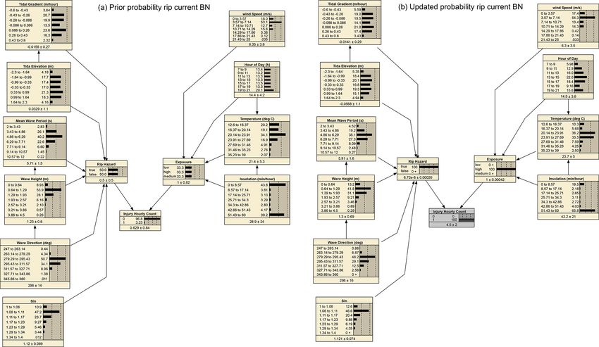
2076                                                    E. de Korte et al.: Bayesian network modelling of surf zone injuries

of people exposed to life-threatening hazards. As a result,       prominent environmental controls, it does not uncover the in-
a beach with a relatively high hazard level could exhibit a       terplay between variables and the relative magnitude of each
low level of risk if the number of beach users is low and         variable. A related challenge based on current research is fil-
vice versa. This way, the level of life risk can be modelled      tering the effect of how water users’ choices are influenced
indirectly by estimating hazard and exposure.                     by environmental conditions (e.g. wave height Hs ). For in-
   There are two primary causes of surf zone injuries (SZIs),     stance Stokes et al. (2017) found that beach morphology type
which can sometimes co-exit at the same beach (Castelle           has an impact on the number of water users. It can also be
et al., 2018): (i) rip currents resulting in drowning incidents   hypothesised that high surf and heavy shore-break waves dis-
and (ii) shore-break waves which can result in, e.g., spine       courage a number of the beachgoers from entering the water,
and shoulder dislocations. Rip currents are intense seaward-      even on warm sunny days, resulting in less exposure. Finally,
flowing narrow currents which can form through different          the respective contributions of hazard and exposure to the
driving mechanisms related to breaking waves (Dalrymple           overall life risk for shore-break waves and rip current are vir-
et al., 2011; Castelle et al., 2018). They form close to the      tually unknown.
shoreline and often extend beyond the surf zone. Therefore           Prediction of SZIs together with a better understanding of
they can transport unsuspecting bathers offshore, who poten-      the interplay between weather and marine conditions and ef-
tially panic and drown (Drozdzewski et al., 2012; Brighton        fect on life risk at the beach could help to better anticipate
et al., 2013). The shore-break wave hazard has received lit-      high-risk days and further improve public safety awareness
tle attention in the literature compared to rip-current hazard.   campaigns on surf zone hazards. This requires a high-order
However, shore-break waves can cause a large number of            statistical approach like a Bayesian network (BN). BNs are
injuries (Puleo et al., 2016), including severe spine injuries    probabilistic graphical models that are based on a joint prob-
(Robbles, 2006). At certain beaches, shore-break waves can        ability distribution of a set of variables with a possible mutual
even be the primary cause of SZIs, e.g. up to 88 % at Ocean       causal relationship. BNs have been previously successfully
City, Maryland (Muller, 2018).                                    used in coastal science, estimating morphological changes,
   Rip flow speed, which is a proxy of rip-current hazard,        changes in wave parameters in the surf-zone and coastal
has been addressed on many beaches through both field mea-        flood risks (Gutierrez et al., 2011; Plant and Holland, 2011;
surements and numerical modelling (see Castelle et al., 2016,     Fienen et al., 2013; Pearson et al., 2017). Stokes et al. (2017)
for a review). In brief, rip flow speed generally increases       compared a BN to a multiple linear regression approach to
with increasing wave height and period (e.g. MacMahan             model exposure, hazard and, in turn, life risk to beach users
et al., 2006), more shore-normal incidence (e.g. MacMa-           at 113 beaches with lifeguards in UK. Even though the mul-
han et al., 2005), generally lower tide levels (e.g. Brander      tiple linear regression method moderately outperformed the
and Short, 2001; Austin et al., 2010; Bruneau et al., 2011;       BN, Stokes et al. (2017) acknowledged the benefits of a BN
Houser et al., 2013; Scott et al., 2014) and more alongshore-     approach to identify the characteristics of high-risk beaches
variable surf zone morphology (Moulton et al., 2017). It is       from a large dataset. More recently, Doelp et al. (2019) used a
also well known that shore-break waves are associated with        BN to predict SZIs on the Delaware coast, which are primar-
steep beaches and longer-period waves (Battjes, 1974; Bal-        ily caused by shore-break waves (Puleo et al., 2016). They
sillie, 1985). In addition, the number of SZIs is also greatly    showed that a BN approach can improve predictions 69.7 %
influenced by the number of beachgoers exposing themselves        of the time but also acknowledged limitations in predicting
to surf zone hazards. Given that warm sunny days with low         anomalous injuries. A BN approach has the potential both to
winds typically result in increased beach attendance (Ibarra,     show good prediction skill to assist decision-making and to
2011; Dwight et al., 2007), it is expected that during such       provide a better understanding of rip-current and shore-break
days the life risk, and thus the number of SZIs, is increased.    hazards.
   Prominent environmental controls on SZIs were identified          In this paper, a dataset (2011–2017) of 442 drowning in-
by comparing the frequency distribution of an environmen-         juries (fatal and non-fatal) and 715 shore-break injuries oc-
tal variable (e.g. significant wave height Hs , tide elevation    curring in boreal summer (15 June–15 September) and corre-
η) during an injury, with the background frequency distri-        sponding environmental conditions along the Gironde coast
bution of that variable (Scott et al., 2014; Castelle et al.,     in southwest France are used to create BNs for rip-current-
2019). The difference between two frequency distributions         related drownings and shore-break injuries. The study area
shows the disproportionate number of conditions that are          and SZI dataset are described in Sect. 2. Section 3 presents
associated with SZIs. At two different beaches along the          the development of the BNs and the method used to train
Atlantic coast of Europe, Scott et al. (2014) and Castelle        them and address their performance. Results are shown in
et al. (2019) showed that the number of drowning inci-            Sect. 4 and are further discussed in Sect. 5 before conclu-
dents increases disproportionately during warm sunny days         sions are drawn.
with light wind, maximising beach attendance, and shore-
normally incident long-period waves, maximising rip-current
activity. Although such analysis provides an indication of the

Nat. Hazards Earth Syst. Sci., 21, 2075–2091, 2021                                https://doi.org/10.5194/nhess-21-2075-2021
E. de Korte et al.: Bayesian network modelling of surf zone injuries                                                          2077

2     Environmental and SZI dataset along the Gironde              2.1.1   SZI data
      coast
                                                                   The SZI dataset used herein is detailed in Tellier et al. (2021).
2.1    Study area                                                  In short, SZIs were recorded by the medical emergency call
                                                                   centre SAMU (Service d’Aide Médicale d’Urgence) of Bor-
The Gironde coast is located in southwest France and               deaux for the Gironde department. Calls from beachgoers
stretches approximately 140 km from the La Salie Beach (La         and lifeguards dealing with drowning or rescues received be-
Teste) in the south to the Gironde Estuary in the north and is     tween January 2011 and November 2017 were used here. Ex-
interrupted by the Arcachon tidal inlet (Fig. 1a). It is a meso-   cluding training calls, duplicates and calls lacking victims,
macrotidal environment with spring tidal range reaching 5 m.       a total of 5022 injuries were collected. Table 2 shows that
Wave conditions vary seasonally with a 99.5 % exceedance           the discrepancy between the total number of injuries and the
significant wave height Hs of 5.6 m, and occasional severe         combined shore-break- and rip-current-related SZIs is due to
storms with Hs > 8 m. Summers are associated with smaller          the large number of calls with insufficient information col-
waves with a mean Hs of around 1.2 m and a dominant W-             lected. Noteworthy is that the 916 surfing-related injuries
NW incidence (Castelle et al., 2019).                              (Table 1) occurring during this period were also disregarded
   The coast is composed of high-energy sandy beaches              for analysis. The reason for this is that a large number of
backed by high and wide coastal dunes. Beaches are inter-          surfer injuries involve collision with other surfers and are
mediate double barred, with deep and more or less regu-            likely influenced by other factors (e.g. surf break quality, surf
lar rip channels incising the intertidal inner bar with an av-     school activity) which are not related to physical hazards.
erage spacing of approximately 400 m (Fig. 1a and b). In-             A SZI was classified as shore-break when the medical file
tense rip currents can flow through the rip channels, with         explicitly stated “shore-break” or a French equivalent. Given
rip flow intensity potentially exceeding 1 m/s even for low-       that along this coast approximately 80 % of the drowning in-
energy (Hs < 1 m) long-period waves (Castelle et al., 2016).       cidents involving bathers are caused by rip currents (Castelle
Rip-current flow is strongly modulated by the tide level,          et al., 2018), rip-related SZIs (drownings) were determined
with maximum rip-current activity occurring between low            if a drowning stage (according to standardised medical clas-
and mid-tide in typical summer wave conditions (Bruneau            sification) was reported in the medical file, with two no-
et al., 2011). In winter, more energetic wave conditions drive     table exceptions. Drownings that were related to shore-break
a more dissipative gently sloping beach face. In contrast, the     waves were classified as shore-break, because they were pre-
upper part of the beach is steeper in summer due to smaller        sumably not associated with rip currents. Similarly, surfing-
waves. Beach slope and rip channel morphology also show            related drownings were excluded as there is no evidence that
a large interannual variability enforced by large interannual      most of the drownings of surfers are related to rip currents.
variability in the wave climate (Dodet et al., 2019). Overall,     Six mutually exclusive classes were found based on activ-
beach states are similar along the coast but with increasingly     ity (see Table 2). Even though the activity was unknown for
steep beach face and deeper and more spaced rip channels           1943 of the SZIs, drowning stage and the shore-break classi-
southwards. Noteworthy is that beach morphology dramati-           fier provided the information to classify some of these SZIs
cally changes along sectors adjacent to the Arcachon lagoon        as shore-break- or rip-related drowning. Amongst the popu-
and Gironde estuary where rip-current activity decreases,          lation, 45 % was male and 33 % female, and for 21 % the sex
but tide-driven currents become substantial (> 0.2 m/s dur-        was not recorded. The population is relatively young, with
ing ebb and flood).                                                43 % between 6 and 19 years old. A slightly elevated number
   The Gironde coast is known for a large population of            of SZIs was found for the age group between 36–45 years old
tourists visiting the beaches, which results in large numbers      (see Fig. 2). This demographic is in line with another, shorter,
of injuries sustained by beachgoers and surfers of all levels      dataset described in Castelle et al. (2018). By far most SZIs
(Fig. 1c) (Castelle et al., 2018; Tellier et al., 2019). Beaches   occurred at Lacanau beach (26 %), which is one of the most
are patrolled by lifeguards during the summer months of July       popular beaches that consequently attracts crowds in summer
and August. Patrolled periods are extended approximately           (see Fig. 2).
from 15 June to 15 September at the busiest beaches. A des-           For the purpose of this study, only summer periods be-
ignated and supervised bathing zone is delimited by two blue       tween 15 June and 15 September were taken for each year
flags. However, many remote beach access paths through             because outside of this period SZIs become extremely rare
coastal dune tracks and many access points are situated on         events, which poses challenges for BN training. In the sum-
unpatrolled sections of beaches, kilometres away from any          mer periods 442 drowning SZIs and 715 shore-break SZIs
lifeguard presence (Castelle et al., 2019).                        were found. This is the final population that was used in the
                                                                   Bayesian network.

https://doi.org/10.5194/nhess-21-2075-2021                                 Nat. Hazards Earth Syst. Sci., 21, 2075–2091, 2021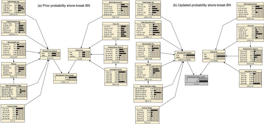
2078                                                       E. de Korte et al.: Bayesian network modelling of surf zone injuries

Figure 1. (a) Location map of the Gironde Coast, southwest France. Black circles indicate municipalities where injuries were reported.
Locations of Truc Vert beach and wave and tide data used in this study are also indicated; (b) aerial photograph of Truc Vert beach at low
tide, exposing rip channels (Vincent Marieu); (c) crowded Lacanau beach in summer during a high tide (Julien Lestage).

Figure 2. Distribution of (a) age and (b) location of SZIs between 8 January 2011 and 18 November 2017. Beaches are ordered from
north (left) to south (right).

2.2    Environmental data                                              lag between the Eyrac tide gauge and beaches of the study
                                                                       area was estimated using tide charts from the Service Hydro-
Environmental conditions were estimated at the time of                 graphique et Océanographique de la Marine (France), result-
each SZI by using a dataset comprising tide, wave and                  ing in an estimated maximum tide elevation error of 0.3 m at
weather data. The dataset is described in detail in Castelle           all sites, which is conservative. A wave model hindcast was
et al. (2019). Hourly weather data were collected at                   used to provide continuous wave conditions at the coast. The
the Météo-France weather station Cap Ferret (Fig. 1a)                  WaveWatch 3 (Tolman, 2014) hindcast was performed on an
from the RADOME (Réseau d’Acquisition de Données                       unstructured grid with a resolution increasing from 10 km
d’Observations Météorologiques Etendu). A tidal component              offshore to 200 m near the coast (Boudière et al., 2013). Wave
analysis of a 3-month time series of continuous, storm-free            conditions were extracted at an in situ directional wave buoy
Eyrac tide gauge data (Fig. 1) was performed to reconstruct            location c. 10 km offshore of Truc Vert at ca. 50 m depth and
a tide level time series at 10 min intervals. The average phase        have been extensively validated with field data (e.g. Castelle

Nat. Hazards Earth Syst. Sci., 21, 2075–2091, 2021                                      https://doi.org/10.5194/nhess-21-2075-2021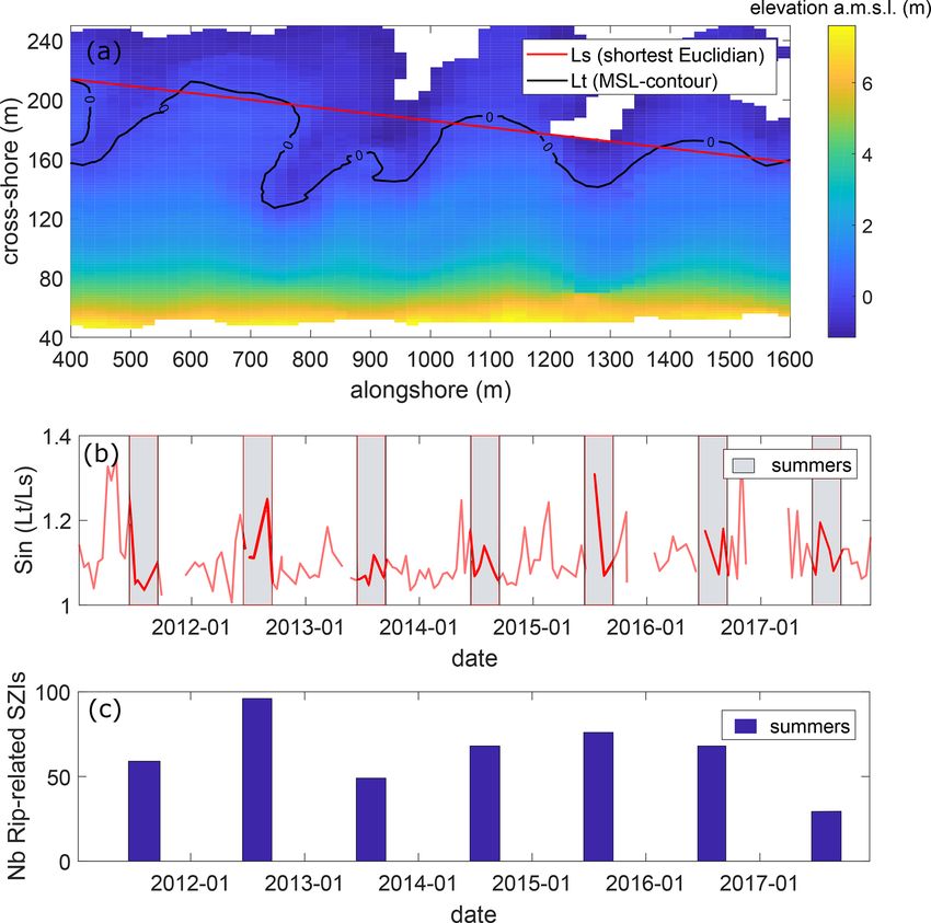
E. de Korte et al.: Bayesian network modelling of surf zone injuries                                                             2079

Table 1. Activity distribution SZIs as indicated in the medical files   defined as
between 8 January 2011 and 18 November 2017.
                                                                              Lt
                                                                        S=       ,                                                 (2)
                   Activity            No. of SZIs                            Ls
                   Swimming                   1229                      where Lt is the true length, and Ls is the shortest Euclidean
                   Surfing                     827                      distance between the first and last points of the contour line
                   Body-boarding                89                      (Fig. 4). A value larger than 1 indicates a high degree of sin-
                   Beach-related               898                      uosity, whereas values close to 1 indicate a low degree of
                   Skim-boarding                36                      sinuosity. Before calculating the sinuosity of the shoreline,
                   Unknown activity           1943
                                                                        a high-pass filter was used to remove sinuous signals larger
                   Total                      5022
                                                                        than 400 m. This was done to filter out larger-scale undulat-
                                                                        ing patterns that are not enforced by the inner-bar rip chan-
Table 2. Post-processed categories to distinguish between rip-          nels (Castelle et al., 2015).
related drownings and shore-break injuries.                                The metocean and topographic data collected at Cap Ferret
                                                                        or near Truc Vert are both located approximately in the centre
            Class                           No. of SZIs                 of the study area. This data were assumed to be representative
                                                                        of wave and weather conditions along the entire study area.
            Swimming (non-drowning)                 282                 When constructing a BN (see next section), probabilities of
            Rip-related drowning                    575
                                                                        a SZI occurrence must be compared to a probability of non-
            Shore-break                             750
                                                                        SZI. Therefore, a discretisation in time is needed. A 1 h time
            Surfing/body-boarding                   916
            Beach-related                           934                 window was chosen to count the number of SZIs. To avoid a
            Unknown                                1565                 spurious distribution of non-SZIs, only daily hours between
            Total                                  5022                 7:00 and 19:00 were used.

                                                                        3     Bayesian networks
et al., 2020). The primary metocean variables used are tidal
elevation (η), significant wave height (Hs ), mean wave period          3.1    Bayes’ theorem and BN structure
(T02 ), wave direction (θ ), temperature (T ), wind speed (U )
and insolation (I ). From tidal elevation, tidal range (TR) and         Bayesian networks (BN) are based on Bayes’ theorem (Korb
tidal gradient (dη) were derived. Maximum, minimum, mean                and Nicholson, 2010). This theorem states that probabilities
and standard deviation summer statistics are summarised in              of a certain event can be updated, given new evidence, and
Table 3.                                                                can be stated as (Bayes, 1763)
   Previous work along this stretch of coast showed, quali-
tatively, the importance of upper beach slope and rip chan-                          P (e|h)P (h)
nel development on shore-break-related injuries and drown-              P (h|e) =                 ,                                (3)
                                                                                         P (e)
ing incidents, respectively (Castelle et al., 2019). To further
quantitatively address this link with the longer dataset used           where P (h|e) is the probability for a hypothesis h, given the
herein, we used monthly to bimonthly topographic surveys                evidence e. In Eq. (3), P (e|h) resembles the likelihood and
performed at Truc Vert beach since 2003 (the reader is re-              P (h) corresponds to the prior probability of h before any ev-
ferred to Castelle et al., 2020, for a detailed description of          idence was given. Dividing the numerator by P (e) is a means
this beach monitoring program). This dataset was used to de-            of normalising, so that conditional probabilities sum to 1. For
rive two morphological metrics. First, the inverse foreshore            example P (h|e) could be the probability of a rip-current haz-
slope (IFS) was calculated as                                           ard, given that the tide was low.
                                                                           A BN is a graphical representation of the probabilistic re-
           1                                                            lations between a set of variables, using Bayes’ theorem to
IFS =          ,                                                 (1)
        tan(β)                                                          describe the relation between variables (Korb and Nicholson,
                                                                        2010). The links between nodes represent the direct depen-
where tan(β) is the beach slope between 1 and 3 m above                 dency between variables (or nodes). A constraint on linking
mean sea level (a.m.s.l.) from a linear regression. To filter           variables is that links cannot return to the beginning node,
out extreme alongshore variations in IFS, the slope was aver-           completing the cycle. Therefore the graphical representation
aged over four cross-shore transects that were systematically           of a BN is often referred to as a directed acyclic graph. If
surveyed during the monitoring programme (Fig. 3).                      there is an arc from variable A to B, variable A is termed
  Sinuosity (S) of the mean sea level iso-contour line was              the parent variable and variable B the child variable. The re-
used to provide a measure rip channel development. It was               lation between variables is often assumed to be causal, but

https://doi.org/10.5194/nhess-21-2075-2021                                      Nat. Hazards Earth Syst. Sci., 21, 2075–2091, 2021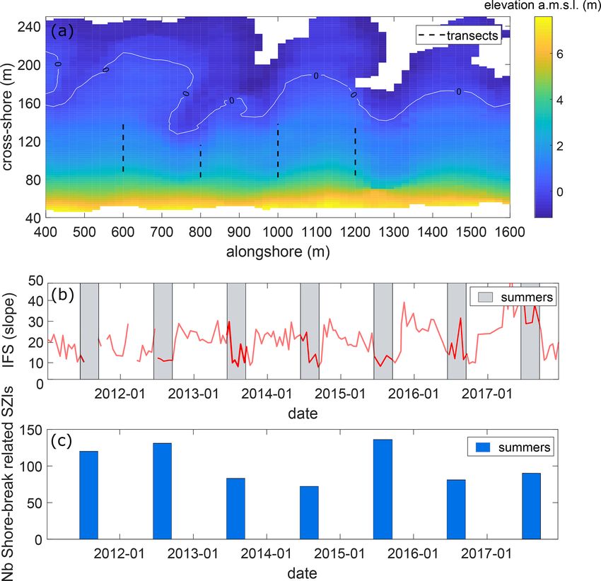
2080                                                        E. de Korte et al.: Bayesian network modelling of surf zone injuries

Table 3. Statistics of environmental conditions of SZI records during summers between 15 June–15 September.

                             Environmental variable             Maximum      Minimum        Mean     Standard
                                                                                                     deviation
                             Significant wave height Hs (m)           3.13        0.23       1.17        0.38
                             Mean wave period T02 (s)                11.64        2.66       6.19        1.94
                             Wave direction θ (◦ )                  340.10      247.30     291.67        7.82
                             Tidal elevation η (m)                    2.21      −2.26      −0.03         1.09
                             Tidal range TR (m)                       4.52        1.64       3.12        0.69
                             Tidal gradient dη (m h−1 )               0.51      −0.51        0.05        0.26
                             Temperature T (◦ C)                     36.23       15.47      25.07        3.36
                             Insolation I (min H−1 )                    60           0      48.17       14.77
                             Wind speed U (m s−1 )                   12.65         1.2       4.56        1.26

Figure 3. (a) Example of a digital elevation model of Truc Vert beach on 29 April 2013, with the colour bar showing elevation above mean
sea level. The four cross-shore transects used to compute the inverse beach slope IFS between 1 and 3 m a.m.s.l. are indicated by the dashed
black lines. (b) Time series of IFS and (c) summer shore-break-related injuries.

is not necessarily the case. Once the structure is established,         there is predictive reasoning, where a value is specified for
relations between variables are quantified according to con-            each input variable. This results in a predicted probability for
ditional probability tables (CPTs), in the case of discrete vari-       a target variable. Secondly, diagnostic reasoning is the other
ables. The probability of a value for a child variable is cal-          type for which, for example, given a SZI the BN can specify
culated for each possible value that the parent variable can            the probability that it was low tide.
take. Given that this is done for all variable nodes in the BN,
two types of probabilistic reasoning become possible. Firstly,

Nat. Hazards Earth Syst. Sci., 21, 2075–2091, 2021                                       https://doi.org/10.5194/nhess-21-2075-2021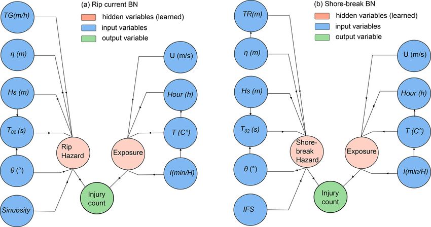
E. de Korte et al.: Bayesian network modelling of surf zone injuries                                                                    2081

Figure 4. (a) Example of a digital elevation model of Truc Vert beach on 29 April 2013, with the colour bar showing elevation above mean
sea level. The red line indicates the shortest Euclidean distance. Time series of (b) sinuosity S and (c) number of summer rip-current-related
drownings.

3.2   Construction of the rip-current- and                               by the inverse foreshore slope (IFS), and the tidal gradient
      shore-break-related BNs                                            (TG) is replaced by tidal range (TR). Such a structure was
                                                                         motivated by the fact that sometimes a simpler and compu-
Constructing a BN requires a trade-off between complexity                tationally less expensive network can be obtained by adding
and predictability. This is determined by the number of vari-            so-called hidden or latent variables that limit the number of
ables chosen, the way variables are discretised and how the              links between variables or the number of variables to in-
variables are linked. In general a simpler model is preferred            clude in the network (Russel and Norvig, 2010, p. 817). In
over a complex model with the same performance, accord-                  this case, we used two hidden exposure and hazard variables
ing to the principle of Ockham’s razor (Jefferys and Berger,             which are known to control life risk and the number of SZIs
1992). In this section we describe the choices that were made            (Stokes et al., 2017).
related to this trade-off, using the BN software package Net-               In order to compare the probability of an injury with the
ica v.6.05 (Norsys, 1998).                                               probability of a non-injury, injuries were counted per hour
   Based on earlier work on the environmental controls on                for all summers. Consequently, the variable injury count was
SZIs in southwest France (Castelle et al., 2019) and some                discretised as a binary variable with two possibilities: no in-
preliminary BN tests, the rip-current BN is made of (i) a haz-           jury or an injury. Where the number of injuries per hour
ard component that depends on hydrodynamic forcing pa-                   exceeded 1, the cases were duplicated proportionally. Often
rameters Hs , T02 , θ, η and dη and a morphological compo-               hidden learned variables tend to be discretised with a small
nent S and (ii) an exposure component that depends on the                number of bins, as they do not have any prior information
hour of the day H , temperature T and hourly insolation I de-            available. After testing both BNs, three dummy bins were
fined as sunshine duration (see Fig. 5). The shore-break BN              chosen for the exposure variable and two dummy bins for
has a similar set-up, but the shoreline sinuosity is replaced            the hazard variable. The number of bins chosen for the in-

https://doi.org/10.5194/nhess-21-2075-2021                                       Nat. Hazards Earth Syst. Sci., 21, 2075–2091, 2021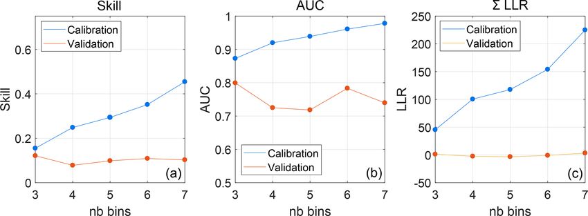
2082                                                         E. de Korte et al.: Bayesian network modelling of surf zone injuries

Figure 5. Bayesian networks for (a) rip-current-related injuries and (b) shore-break injuries. Both BNs are defined by input variables, hidden
variables, an output variable and their linkages.

put variables determines the performance of the model to a               dataset. After 10 folds, mean values of performance metrics
larger extent. Therefore, different discretisation options were          were taken to evaluate the performance of the BN.
tested, keeping an equal bin width. This is shown in Sect. 3.4.
                                                                         3.4    BN performance metrics
3.3    Bayesian network training
                                                                         Different performance metrics were used to address BN pre-
The probability tables of the hidden variables were calcu-               dictive performance. Here we used three relevant metrics:
lated by using an algorithm that calculates the most likely              skill sk, log likelihood ratio LLR and area under ROC (re-
distribution of the data, given the probability distributions of         ceiver operating characteristic) AUC.
the other variables. The expectation maximisation (EM) al-                  Skill was adapted from Fienen and Plant (2015) and was
gorithm is widely used in BNs to determine the most likely               computed as
model given the data (Russel and Norvig, 2010). In a similar
manner the algorithm finds the most likely value for occa-                           σe2
                                                                         sk = [1 −       ] × 100 %,                                       (4)
sionally missing data. The algorithm proceeds in the direc-                          σo2
tion of the steepest gradient to find the minimum negative log
likelihood for a model, given the data. The number of bins               where σe is the mean squared error between observations and
used to discretise variables in the BN determines how well               the BN forecast, and σo is the variance of observations. The
data are described. The larger the number of bins, the bet-              skill metric in Eq. (4) expresses how close predictions of
ter it describes the data until the point where there might be a         an injury match with observations of an injury, with sk = 1
bin for each value. On the other hand, a larger number of bins           meaning perfect prediction.
degrades the prediction skill of the BN, as it becomes harder               Because skill is not an optimal measure for binary output
to predict the correct bin. A BN might be trained slightly               variables, the AUC (area under ROC curve) was chosen as a
differently from one run to another, because it is a proba-              complementary metric (Marcot, 2012). AUC is based on the
bilistic process. Therefore, we used K-fold cross-validation             ratio between the true positive predictions of the BN and the
to eliminate any bias that single model runs might hold. After           false positive predictions. Figure 6a shows the sensitivity on
Fienen and Plant (2015), Gutierrez et al. (2015), and Pearson            the y axis (true positive rate) and the specificity on the x axis
et al. (2017) the cases were separated into k random parti-              (false positive rate) of a typical ROC curve from one of the
tions, where n − n/k cases were used for training and cal-               model runs. If the dashed random classification line is equal
ibration, and n/k cases were left out for testing/validation.            to the ROC curve, this indicates that the model is not able to
We used k = 10 so that test cases make up 10 % of the total              distinguish an injury from a non-injury. This corresponds to

Nat. Hazards Earth Syst. Sci., 21, 2075–2091, 2021                                        https://doi.org/10.5194/nhess-21-2075-2021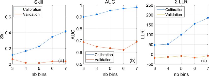
E. de Korte et al.: Bayesian network modelling of surf zone injuries                                                            2083

                                                                    new evidence. V (F ) and V (F |O) are calculated as

                                                                               N
                                                                               X
                                                                    V (F ) =          p(fj )(fj − E(fj ))2 ,                      (7)
                                                                               j =1
                                                                               M X
                                                                               X N
                                                                    V (F ) =              p(fj |oi )(fj − E(fj |oi ))2 ,          (8)
                                                                               i=1 j =1

                                                                    where p(fj ) is the prior probability of the j th forecast, fj is
                                                                    the current value of the j th forecast, E(fj ) is the expected
                                                                    value predicted by the BN of the j th forecast, p(fj |oi ) is
                                                                    the predicted value of the j th forecast given the ith evidence
                                                                    case, E(fj |oi ) is the predicted value of the j th forecast given
                                                                    the ith evidence case, M represents the number of evidence
Figure 6. Receiver operating characteristic curve (ROC) of the      data and N is the number of predictions.
shore-break BN of one of the fold runs.

                                                                    4     Results
AUC = 0.5. Figure 6b shows the confusion matrix on which            4.1    BN performance
the sensitivity and specificity are based.
   The third metric is the log likelihood ratio (LLR), adapted      To find the best BNs, a varying number of bins was tested
from Plant and Holland (2011) and Fienen et al. (2013). The         to evaluate the trade-off between calibration and validation.
LLR compares the prior probability of an injury with the pos-       For calibration, the BN was trained to make predictions of
terior probability of a prediction, given the evidence (the in-     an injury based on the input variables of 90 % of the train-
put variables), which reads                                         ing cases. For validation, predictions of an injury were made
                                                                    based on the input variables of the 10 % left-out cases. Gen-
LLR = log10 (p(Fi |Oj )Fi =Oj0 ) − log10 (p(Fi )Fi =Oj0 ),   (5)    erally an increase in level of definition, i.e. number of bins,
                                                                    leads to a decrease in predictive capability and vice versa
                                                                    (Fienen and Plant, 2015; Fienen et al., 2013). Figures 7 and
where Fi is a forecast, in this case of a SZI, and Oj is an         8 show performance metrics for both the shore-break and rip-
independent observation that was withheld from the fore-            current BNs, respectively, as a function of the number of bins
cast (e.g. a tidal elevation of −2.0 m). The LLR expresses          for the input variables.
the change in likelihood due to certain evidence in the form           It can be observed that the shore-break BN performs
of observations. A LLR that exceeds zero indicates that the         slightly better than the rip-current BN, as all performance
BN offers a better forecast than the prior probability. A LLR       metrics score better. Calibration results of the BNs are fair,
that is lower than zero indicates that the prior probability is a   with sk and AUC ranging from 0.15–0.43 and 0.89–0.98, re-
better forecast than the BN forecast. The LLR can be calcu-         spectively. Validation sk is smaller and ranges from 0.078–
lated for each predicted case andPeach variable and can then        0.12 and 0.035–0.06 for the shore-break and rip-currents
be summed over the entire BN ( LLR). The LLR penalises              BNs, respectively. Validation AUCs are better, ranging from
wrong but confident predictions more than wrong predictions         0.71–0.8 and 0.63–0.68 for the shore-break and rip-current
that are uncertain (Plant and Holland, 2011; Pearson et al.,        BNs, respectively. The sum of the LLR is systematically
2017). Therefore, it is a suitable metric to verify whether the     smaller than 0 for the validation of both BNs. This is either
BN is over-fitting or not.                                          an indication that the prior estimate is on average better than
   Finally, in order to address how each input variable influ-      the prediction of the model or that there are anomalous cases
ences the target variable (SZI), the percentage of variance         where the wrong but confident prediction is heavily punished
reduction Vr that was caused by updating the BN based on            by highly negative LLR values that result in a negative or
the evidence was computed as                                        near-zero LLR sum.
                                                                       Tables 4 and 5 show that, depending on the number of bins
                                                                    chosen, model predictions are better than the prior probabil-
       V (F ) − V (F |O)
Vr =                     × 100 %,                            (6)    ity estimate 62.21 %–79.9 % of the time. When five bins are
             V (F )                                                 chosen for the rip-current BN, 79 % of the time the model
                                                                    prediction is of added value. When five bins are chosen for
where V (F ) is the variance of a forecast prior to any evi-        the shore-break BN, 72 % of time the model prediction per-
dence, and V (F |O) is the variance of the forecast, given the      forms better. This shows that the negative and near-zero sums

https://doi.org/10.5194/nhess-21-2075-2021                                  Nat. Hazards Earth Syst. Sci., 21, 2075–2091, 2021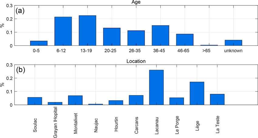
2084                                                         E. de Korte et al.: Bayesian network modelling of surf zone injuries

Figure 7. Performance metrics of shore-break BN as a function of the number of bins P
                                                                                    of the input variables and for validation and calibration:
(a) skill sk, (b) area under ROC curve AUC and (c) the summed log likelihood ratio LLR.

Figure 8. Performance metrics of rip-current BN as a function of the number of bins P
                                                                                    of the input variables and for validation and calibration:
(a) skill sk, (b) area under ROC curve AUC and (c) the summed log likelihood ratio LLR.

Table 4. The percentage of LLR > 0 for rip-current SZIs, indicating      Table 5. The percentage of LLR > 0 for shore-break SZIs, indi-
whether the prediction of the model is better than the prior proba-      cating whether the prediction of the model is better than the prior
bility.                                                                  probability.

               No. of bins    Prediction rip-current                                     No. of bins   Prediction shore-break
                                 SZIs (% LLR > 0)                                                         SZIs (% LLR > 0)
               Three bins                   73.86 %                                      Three bins                   70.18 %
               Four bins                    77.30 %                                      Four bins                    70.08 %
               Five bins                    79.90 %                                      Five bins                    72.56 %
               Six bins                     61.60 %                                      Six bins                     65.10 %
               Seven bins                   62.21 %                                      Seven bins                   69.50 %

                                                                         is increased from three to four, a small decrease in sk and
of the LLR displayed in Figs. 7 and 8 must be caused by
                                                                         AUC can be noticed. However, a further increase in the num-
anomalous events (the remaining percentages) that are confi-
                                                                         ber
                                                                         P of bins does not significantly lead to worse sk, AUC or
dently predicted wrong.
                                                                            LLR. AUC and sk show a small increase at six bins for the
   The number of bins was varied from three to seven bins
                                                                         shore-break BN (Fig. 7a, b) and at six to seven bins for the
to choose the best trade-off between complexity and accu-
                                                                         rip BN (Fig. 7). Contrary
                                                                                               P to what is generally observed, val-
racy. Only the number of input variable bins was adjusted,
                                                                         idation sk, AUC and LLR did not drop dramatically when
keeping the output variables exposure, hazard and injury the
                                                                         complexity was increased. However, the percentage LLR > 0
same. In general, an increase in the number of bins leads to
                                                                         did drop for both BNs, when increasing the number of bins,
a better descriptive capability and a worse predictive capa-
                                                                         which is in line with expectations.
bility (Fienen and Plant, 2015). When the number of bins

Nat. Hazards Earth Syst. Sci., 21, 2075–2091, 2021                                        https://doi.org/10.5194/nhess-21-2075-2021
E. de Korte et al.: Bayesian network modelling of surf zone injuries 2085
4.1.1 Input variable sensitivity towards higher mean wave periods (T02 ) and a slight in-
crease in probabilities of larger wave heights (Hs ). Further-
Figure 9a shows the sensitivity of the shore-break BN to the more, temperature, hour of the day and insolation show a pro-
input variables (six bins) and to the hidden variables expo- nounced shift towards higher temperatures, less cloud cover
sure and shore-break hazard. For the shore-break BN, the and the afternoon between 14:00 and 16:30. Noteworthy is
learned variable exposure (Vr = 23.5 %) has the strongest in- that when the BN was updated for larger wave heights, the
fluence followed by the shore-break hazard variable (Vr = probability of a shore-break-related injury increased. How-
10.9 %). This suggests that exposure of water users has a ever, when the BN was updated with the evidence of an in-
more dominant control on the injury count than the shore- jury, intermediate wave height bins 0.75–1.5 and 1.5–2.25 m
break hazard forcing variables. This is also reflected in showed increased probability. This supports our hypothesis
Fig. 9b, where the hour of the day, temperature and insolation that large shore-break waves (Hs > 2.5 m) can discourage
have larger values for Vr. These variables are followed by bathers from entering the water, which results in fewer SZIs
tide elevation, which is the most important shore-break haz- despite that the shore-break hazard is increased.
ard control (Vr = 0.17 %). Consequently, mean wave period A similar scenario analysis was performed for the rip-
(Vr = 0.07 %), tidal range (Vr = 0.06 %), significant wave current BN. Figure 11a shows prior probabilities of the rip-
height (Vr = 0.05 %) and wind speed (Vr = 0.039 %) fol- current BN. The rip-current BN shows that according to
low. The inverse foreshore slope IFS averaged over four the prior probability a shore-break-related injury (5.60 %)
profiles distributed along the coast has a noticeable impact is more likely than a rip-current-related (fatal or non-fatal)
(Vr = 0.065 %) on the shore-break hazard. Wave direction is drowning (3.23 %). Figure 11b shows the updated probabil-
least sensitive to the injury count with Vr = 0.025 %. ity distributions for the rip-current BN, given that there is a
Figure 9c shows the sensitivity of the rip-current BN to 100 % chance of an injury. Although the probability distribu-
the input variable (seven bins) including the hidden vari- tion of the central bins of tidal gradients is similar in pattern,
ables exposure and rip-current hazard. Rip-current exposure extreme tidal gradients (|dη| > 0.43 m/h) show an increase in
(Vr = 17.6 %) and hazard (Vr = 15.4 %) have similar influ- probability by about 50 %. Larger tidal gradients (both neg-
ence, even though parents of exposure (insolation, tempera- ative and positive) show a slight increase in probability, sup-
ture and hour) are more dominant in Fig. 9d. This suggests porting the hypothesis that a rapid change in tidal elevation
that it is the combined effects of input variables that cause can surprise water users by driving the rapid onset of rip-
a rip current (e.g. tide, wave direction and wave height) that current activity. Rip-current-related drownings are slightly
have a strong influence on the occurrence of drowning inci- more likely to occur when tides are low, with increased prob-
dents. This is different from what was observed for the shore- abilities for larger Hs and T02 . Wave direction shows a small
break BN. Within the exposure variables, the most sensitive increase in drowning probability for the NW-oriented direc-
for the rip-current BN are insolation (Vr = 1.67 %), tempera- tions. More sinuous shorelines (larger S values) show slightly
ture (Vr = 1.7 %) and hour of the day (Vr = 1.56 %). Within increased probability of rip-current-related drowning (see
hazard-related variables Hs and T02 have the highest Vr with for S > 1.23 in Fig. 11b), suggesting that more alongshore-
0.36 % and 0.26 %, closely followed by wave direction with variable surf zone morphology increases the rip-current haz-
0.25 %, suggesting that incident wave conditions are the most ard. Wind speed has only little influence, although low wind
important control on rip-current hazard. Shoreline sinuosity speeds are slightly more likely during a drowning incident.
S reduces variance by 0.065 %. Interestingly enough, the per- Furthermore, the hour of the day shows a distribution that
centage of variance reduction of exposure variables is of sim- corresponds with the expected beach attendance. However,
ilar magnitude, although with different ordering, in both haz- there is a disproportionate peak in the evening between 19:00
ards (Fig. 9b, d). and 21:00. Furthermore, the highest peak is earlier between
13:00–15:00 (Fig. 11b) compared to shore-break injuries,
4.2 Scenario analysis although the bins slightly overlap (14:00–16:33, Fig. 10b).
Temperature and insolation show comparable patterns to the
Apart from the predictive ability of a BN, probabilistic sce- shore-break BN, with warm sunny days between 20–28 ◦ C
nario analysis can be a useful tool to understand how multiple having the highest probability.
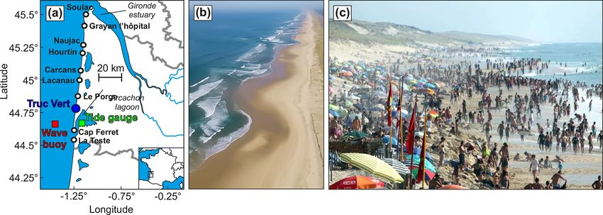
variables interact. Figure 10a shows the prior joint probabil- Other rip-current BN scenarios were tested, providing in-
ity distribution of the shore-break BN without updating based sight into variable interactions. For instance, an interaction
on any evidence. The two hidden variables, exposure (three between the magnitude of shoreline sinuosity S and wave
bins) and hazard (two bins) do not contain any prior infor- angle of incidence was explored, given average wave con-
mation and thus have equal probabilities for each bin. Fig- ditions (wave height and period) and a 100 % chance that
ure 10b shows the joint probability distribution for a trained there was a rip hazard (Fig. 12a and b). It can be ob-
shore-break BN updated for the evidence that there was a served that a low beach sinuosity (1–1.06) is correlated
shore-break SZI. In the latter, the distribution of tidal ele- with higher probabilities for the shore-normally incident
vation shifts towards high tide. Additionally, there is a shift waves (around 279◦ ), while large beach sinuosity is associ-
https://doi.org/10.5194/nhess-21-2075-2021 Nat. Hazards Earth Syst. Sci., 21, 2075–2091, 20212086 E. de Korte et al.: Bayesian network modelling of surf zone injuries
Figure 9. Variance reduction (Vr) without hidden learned variables for the shore-break BN (seven bins) (a) with hidden learned variables and
(b) without learned hidden variables and for the rip-current BN (six bins) (c) with hidden learned variables and (d) without hidden learned
variables.
ated with a larger probability for more NW angles of inci- simple beach morphology parameters S and IFS were derived
dence (295.43–311.57◦ ). This indicates that for reasonably from a single site (Truc Vert). Summer beach morphologies
alongshore-uniform beaches more shore-normally incident surveyed along different beaches distributed along the coast
wave conditions are required to have a rip-current hazard, should help improve IFS and S estimation and, in turn, pre-
which is not necessary for rip-channelled beaches. diction of rip-current drowning incidents and shore-break-
related injuries. Similarly, optical satellite images should be
explored to derive beach sinuosity S at the different beaches
5 Discussion along the coast (Castelle et al., 2021). As indicated earlier,
an estimation of beach attendance or water users should also
5.1 BNs as a predictive tool for SZIs improve BN predictive ability. Therefore, at this stage other
tools should be used for life-risk prediction, like for instance
Two separate BNs were created for shore-break SZIs and rip- models based on simple correlations between meteorological
current SZIs. This allowed use of different beach morphol- and oceanographic conditions and the incidence (Lushine,
ogy metrics based on prior understanding of the physics of 1991; Lascody, 1998; Dusek and Seim, 2013; Scott et al.,
shore-break waves and rip-current dynamics. In addition, two 2014), on the numerical modelling of rip flow speed (Austin
hidden variables (exposure and hazard) were introduced for et al., 2013), or on the combination of video images and nu-
both BNs to decrease the number of connections and increase merical modelling (Jiménez et al., 2007). Recently, using the
BN efficiency. Doelp et al. (2019) used population data to same SZI dataset, a logistic regression model was found to
test a SZI ratio, normalised by the population, in addition to predict the risk of drowning along the Gironde coast up to
the binary injury likelihood. Although results were not dra- 3 d in advance with good skill (Tellier et al., 2021).
matically improved in Doelp et al. (2019), including accurate Lastly, there were 1565 unknown injuries that could not be
water user data should improve BN model predictions along attributed to either a shore-break- or a rip-current-related in-
the Gironde coast. However, such data do not exist and will jury. Theoretically, a well-trained BN could estimate which
require future research effort. of the SZIs is more likely based on the environmental condi-
Performance metrics indicate that the BNs improve prior tions. However, since the BNs are still limited in prediction,
estimates, but that BNs still have a significant percentage of this should be explored in the future using improved BNs.
wrong but confident predictions. This is due to over-fitting, Such a BN could help to retrospectively improve SZI statis-
which is a common issue with training a BN on rare events tics along surf coasts.
(unbalanced dataset) (Cheon et al., 2009). When the primary
objective of a BN is prediction rather than description, a syn- 5.2 Environmental controls on SZIs and implications
thetic dataset can be created with an even distribution of for beach safety management
events, although it degrades the BN descriptive ability. A
similar suggestion to cope with this problem is to remove In other studies frequency analysis was used to identify dis-
anomalous confident but wrong predictions (Doelp et al., proportionate environmental conditions during SZIs (Scott
2019). Another issue limiting the BN predictive ability is that et al., 2014; Castelle et al., 2019). Some of the BN results are
Nat. Hazards Earth Syst. Sci., 21, 2075–2091, 2021 https://doi.org/10.5194/nhess-21-2075-2021E. de Korte et al.: Bayesian network modelling of surf zone injuries 2087 Figure 10. (a) Prior probability distribution of the shore-break BN. (b) Updated probability distribution where the probability of an injury occurring was set to 100 %. Figure 11. (a) Prior probability distribution of the rip-current BN; (b) updated probability distribution of the rip-current BN when the probability of an injury occurring was set to 100 %. https://doi.org/10.5194/nhess-21-2075-2021 Nat. Hazards Earth Syst. Sci., 21, 2075–2091, 2021
2088                                                        E. de Korte et al.: Bayesian network modelling of surf zone injuries

Figure 12. (a) Scenario with low sinuosity resulting in more shore-normal wave direction (around 279◦ ) with the rip-current BN. (b) Scenario
with medium sinuosity resulting in more obliquely incident (NW) wave conditions with the rip-current BN.

essentially in line with previous work. In short, more SZIs are          and Gironde estuary where tide-driven currents, which are
observed for warm sunny days with light winds. Rip-current-              maximised during ebb and flood (large |dη|), can be intense.
related drowning incidents increase with increasing incident                In addition to the primary environmental controls on SZIs,
wave energy (height and period), more shore-normal inci-                 in this study for the first time it was possible to identify the
dence and lower tide level. In contrast, shore-break-related             interaction between multiple input variables. For instance,
injuries are sustained at high tide levels and moderate wave             it was found that it is the combined effects of tide eleva-
height. In addition to previous work, here we proposed a                 tion, wave direction and wave height that control rip-current
method to quantify the role of beach morphology in SZIs.                 hazard. In other words, even if you have shore-normally in-
Beach sinuosity S, which is a measure of the alongshore vari-            cident waves near low tide, if wave height is very small,
ability of surf zone morphology, and inverse beach slope IFS             there is no hazard and consequently a low probability of
were found to influence the occurrence of rip-current-related            rip-current-related drownings. Such interactions, which were
drowning incidents and shore-break-related injuries, respec-             not possible to address in previous work (Scott et al., 2014;
tively. These results are in agreement with current knowledge            Castelle et al., 2019), are in line with the understanding of
of rip flow intensity increasing with increasingly alongshore-           rip flow response to wave and tide conditions (Castelle et al.,
variable surf zone morphology (Moulton et al., 2017) and                 2016). Our scenario analysis also indicates that, for reason-
shore-break waves occurring for steeper beach face (Battjes,             ably alongshore-uniform beaches, more shore-normally inci-
1974; Balsillie, 1985). We also found that rapid, positive or            dent wave conditions are required to have a rip-current haz-
negative, change in tide level elevation (large dη) increase             ard compared with rip-channelled beaches. This is also in
the probability of drowning incidents, with no difference be-            line with observations and model outputs showing that, for
tween ebb and flood. Given that tide-driven current is negli-            the same obliquely incident wave conditions, rip cell cir-
gible compared with rip currents along most of the beaches               culation is transformed into an undulating, less hazardous
in southwest France, this suggests that rapid changes in tidal           longshore current for weakly (small S) alongshore-variable
elevation driving the rapid onset of rip-current activity can            surf zone morphology, while rip cell circulation can be sus-
surprise unsuspecting bathers and carry them offshore. How-              tained for deep rip channels (MacMahan et al., 2008; Dal-
ever, another explanation is that some of the drowning in-               rymple et al., 2011). This shows that BNs including a pre-
cidents occurred in sectors adjacent to the Arcachon lagoon              defined hidden hazard variable can provide insight into the
                                                                         influence of the primary input variables and their interactions

Nat. Hazards Earth Syst. Sci., 21, 2075–2091, 2021                                        https://doi.org/10.5194/nhess-21-2075-2021
E. de Korte et al.: Bayesian network modelling of surf zone injuries 2089
on the hazard posed. Therefore, it could also be applied to ber of severe injuries sustained in shore-break waves along
other injuries, e.g. related to surfing activity, for which the the Gironde coast. We advocate that such BNs should be de-
causes (e.g. environmental, behavioural) and their interplay veloped in parallel with other risk predictors showing high
are poorly understood. predictive skill but providing much less diagnostic capability
Studies addressing the environmental controls on shore- (Tellier et al., 2021).
break-related SZIs are scarce (Puleo et al., 2016; Doelp et al.,
2019) compared to drowning studies. The shore-break BN
developed herein for the Gironde coast suggests that the Data availability. The wave buoy data are publicly available
predicted decrease in exposure for Hs > 2.5 m, representing through the French Candhis network operated by CEREMA.
heavy shore-break waves at the shoreline, is thought to dis- Weather station and tide gauge data are available from the Météo
courage beachgoers from entering the water near high tide. France Radome network and the SHOM, respectively. Wave hind-
cast is available from the MARC platform (Modelling and Analy-
Importantly, this was not observed for rip-current-related
sis for Research in Coastal environment) at https://marc.ifremer.fr
drownings, which have a tendency to occur at low tide with (MARC, 2019). The injury data collected on beaches are not pub-
the inner surf zone located on a much more gently sloping licly available due to restriction from the French National Commit-
part of the beach profile. We hypothesise that in such less tee for the Protection of Data Privacy.
adverse conditions, beachgoers are less discouraged to en-
ter the water, as opposed to facing large shore-break waves.
However, further investigation on beachgoer behaviour in the Author contributions. BC and ET designed the research presented
presence of shore-break waves is required to test this hypoth- here. EdK designed the experiments, performed the modelling ex-
esis. This will also involve estimation of beachgoer affluence periments and analysed all the results. BC and ET consulted on
and estimation of the number of people in the surf exposing the experiments. EdK prepared the manuscript, and BC and ET re-
themselves to the physical hazards. viewed and edited the manuscript.
In addition, our variable sensitivity analysis indicates the
shore-break-related injuries are more controlled by exposure-
related variables than by hazard-related variables, contrary to Competing interests. The authors declare that they have no conflict
rip-current-related drowning for which life risk is approx- of interest.
imately equally distributed between hazard and exposure.
This indicates that shore-break injuries are more likely to
Disclaimer. Publisher’s note: Copernicus Publications remains
occur during busy days, whether moderate or heavy shore-
neutral with regard to jurisdictional claims in published maps and
break conditions are present. In contrast, the presence of in- institutional affiliations.
tense rip currents is critical to drowning incidents.
Acknowledgements. We thank Bruno Simonnet, who contributed to
6 Conclusions the injury data collection. Constructive suggestions to improve read-
ability by Rieke Santjer were much appreciated. This study includes
A Bayesian network (BN) approach was used to model the beach monitoring study site of Truc Vert labelled by the Service
life risk and the controls and interactions of environmental National d’Observation (SNO) Dynalit, whose surveys are finan-
(metocean and morphological) data on SZIs along a high- cially supported by Observatoire de la Côte Aquitaine (OCA) and
energy meso-macrotidal coast where shore-break and rip- SNO Dynalit.
current hazards co-exist. In line with previous work, the BNs
show limited predictive skill. Although the shore-break and
rip-current BNs improve prior estimates, they still have a Financial support. This research has been supported by the Agence
large percentage of wrong but confident predictions, which Nationale de la Recherche (grant no. ANR-17-CE01-0014).
is not tenable for life-risk prediction on beaches. However,
the BNs provide fresh insight into the different environmen-
Review statement. This paper was edited by Mauricio Gonzalez
tal controls, their interactions, and their respective contribu-
and reviewed by Christopher Stokes and Jose A. Jiménez.
tion to hazard and exposure. For the first time, the respective
contributions of exposure and hazards to the overall life risk
were quantified, showing the shore-break-related injuries are
more controlled by the exposure than by hazard, contrary to
References
rip-current-related drowning for which contributions are ap-
proximately equal. These results can guide the future devel- Austin, M., Scott, T. M., Brown, J. W., Brown, J. A., MacMahan,
opment, or modification, of public education messaging, par- J. H., Masselink, G., and Russell, P.: Temporal observations of
ticularly on shore-break hazard, which has received little at- rip current circulation on a macro-tidal beach, Cont. Shelf. Res.,
tention so far compared to rip currents, despite the large num- 30, 1149–1165, https://doi.org/10.1016/j.csr.2010.03.005, 2010.
https://doi.org/10.5194/nhess-21-2075-2021 Nat. Hazards Earth Syst. Sci., 21, 2075–2091, 2021You can also read