Winter drainage of surface lakes on the Greenland Ice Sheet from Sentinel-1 SAR imagery
←
→
Page content transcription
If your browser does not render page correctly, please read the page content below
The Cryosphere, 15, 1587–1606, 2021
https://doi.org/10.5194/tc-15-1587-2021
© Author(s) 2021. This work is distributed under
the Creative Commons Attribution 4.0 License.

Winter drainage of surface lakes on the Greenland Ice Sheet from
Sentinel-1 SAR imagery
Corinne L. Benedek and Ian C. Willis
Scott Polar Research Institute, University of Cambridge, Cambridge CB2 1ER, UK

Correspondence: Corinne L. Benedek (clb90@cam.ac.uk)

Received: 10 March 2020 – Discussion started: 14 May 2020
Revised: 3 February 2021 – Accepted: 4 February 2021 – Published: 1 April 2021

Abstract. Surface lakes on the Greenland Ice Sheet play a       1   Introduction
key role in its surface mass balance, hydrology and biogeo-
chemistry. They often drain rapidly in the summer via hy-       Lakes form each summer on the surface of the Greenland Ice
drofracture, which delivers lake water to the ice sheet base    Sheet (GrIS), particularly in the upper ablation and lower ac-
over timescales of hours to days and then can allow melt-       cumulation areas (McMillan et al., 2007; Selmes et al., 2011;
water to reach the base for the rest of the summer. Rapid       Liang et al., 2012; Pope et al., 2016; Williamson et al., 2017).
lake drainage, therefore, influences subglacial drainage evo-   They enhance melt rates by reducing albedo (Lüthje et al.,
lution; water pressures; ice flow; biogeochemical activity;     2006; Tedesco et al., 2012), store water and delay its deliv-
and ultimately the delivery of water, sediments and nutri-      ery to the ocean (Banwell et al., 2012; Leeson et al., 2012;
ents to the ocean. It has generally been assumed that rapid     Arnold et al., 2014), and collect nutrients – the products of
lake drainage events are confined to the summer, as this is     surface inorganic and organic chemical processes (Musilova
typically when observations are made using satellite optical    et al., 2017; Lamarche-Gagnon et al., 2019). Many lakes
imagery. Here we develop a method to quantify backscat-         drain over the summer (Selmes et al., 2013; Williamson et al.,
ter changes in satellite radar imagery, which we use to doc-    2017), sometimes slowly by overtopping their basins and in-
ument the drainage of six different lakes during three win-     cising a channel (Hoffman et al., 2011; Tedesco et al., 2013;
ters (2014/15, 2015/16 and 2016/17) in fast-flowing parts of    Koziol et al., 2017) but often rapidly by hydrofracturing from
the Greenland Ice Sheet. Analysis of optical imagery from       the surface to the base of the ice sheet (Das et al., 2008; Doyle
before and after the three winters supports the radar-based     et al., 2013; Tedesco et al., 2013; Stevens et al., 2015; Chud-
evidence for winter lake drainage events and also provides      ley et al., 2019). The rapid drainage of a lake may trigger the
estimates of lake drainage volumes, which range between         opening of crevasses and the generation of moulins (Hoff-
0.000046 ± 0.000017 and 0.0200 ± 0.002817 km3 . For three       man et al., 2018) or the drainage of other lakes (Christof-
of the events, optical imagery allows repeat photoclinom-       fersen et al., 2018) through ice dynamic coupling. Rapid lake
etry (shape from shading) calculations to be made show-         drainage provides a major shock to the ice sheet as millions
ing mean vertical collapse of the lake surfaces ranging be-     of cubic metres of water are delivered to the bed in a few
tween 1.21 ± 1.61 and 7.25 ± 1.61 m and drainage volumes        hours, and the resultant fracture may permit meltwater to
of 0.002 ± 0.002968 to 0.044 ± 0.009858 km3 . For one of        reach the bed for the rest of the summer. This lake drainage
these three, time-stamped ArcticDEM strips allow for DEM        and subsequent water input generates a radiating subglacial
differencing, which demonstrates a mean collapse depth of       water “blister” beneath the draining lake, which evolves into
2.17 ± 0.28 m across the lake area. The findings show that      a conduit in the down-hydraulic-potential direction allowing
lake drainage can occur in the winter in the absence of ac-     the lake water and subsequent meltwater to be evacuated (Pi-
tive surface melt and notable ice flow acceleration, which      mentel and Flowers, 2010; Tsai and Rice, 2010; Dow et al.,
may have important implications for subglacial hydrology        2015). High water pressures are generated transiently during
and biogeochemical processes.                                   lake drainage (Banwell et al., 2016), lifting the ice sheet off
                                                                the bed and increasing temporarily its sliding velocity (Das

Published by Copernicus Publications on behalf of the European Geosciences Union.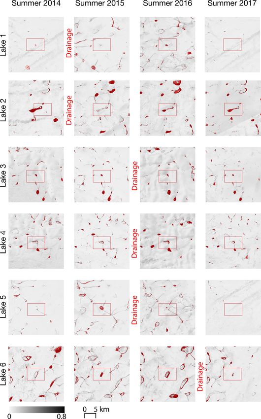
1588                         C. L. Benedek and I. C. Willis: Winter drainage of surface lakes on the Greenland Ice Sheet

et al., 2008; Doyle et al., 2013; Tedesco et al., 2013; Stevens
et al., 2015; Chudley et al., 2019). The subsequent evolution
of the subglacial conduit may lower water pressures (Schoof,
2010; Hewitt, 2013; Werder et al., 2013; Banwell et al., 2016)
and reduce sliding speeds, often below pre-drainage values as
a result of temporary increases in basal hydraulic efficiency
(Bartholomew et al., 2010).
   Rapid lake drainage and subsequent meltwater influx also
alter subglacial biogeochemistry as large volumes of oxy-
genated water containing surface microbial taxa and inor-
ganic and organic nutrients replace wintertime anoxic wa-
ters and associated microbes, shifting subglacial redox po-
tential and associated biogeochemical pathways (Wadham
et al., 2010; Shade et al., 2012). Thus, lake drainage events
influence the quantity and quality of water issuing from
the ice sheet, although their effects are superimposed on
the larger-scale atmospheric controls on melt patterns and
runoff. They can produce small floods that flush out sedi-
ments (Bartholomew et al., 2011); raise levels of phosphorus,     Figure 1. Study area within the context of the Greenland Ice Sheet
nitrogen and sulfate in proglacial streams (Hawkings et al.,      (inset). Distribution of all surface lakes detected from optical im-
2016; Wadham et al., 2016); and mark a transition from net        agery, with the six winter draining lakes highlighted (red numbers,
subglacial methane production and proglacial export during        in chronological order of drainage), which are shown in more detail
winter to consumption with little or no export in the summer      in Fig. 6. The base map is a composite image showing the maxi-
(Dieser et al., 2014).                                            mum NDWIice observed for each pixel in Landsat 8 optical images
   Much of what we know about the locations, timings and          over the course of all summers from 2014 to 2017. The outline of
magnitudes of rapid lake drainage events comes from the           Greenland is from OpenStreetMap (© OpenStreetMap contributors
analysis of optical satellite imagery (Box and Ski, 2007;         2019; distributed under a Creative Commons BY-SA License).
McMillan et al., 2007; Sneed and Hamilton, 2007; Lee-
son et al., 2013; Moussavi et al., 2016; Pope et al., 2016;
                                                                     Here we develop an algorithm to examine spatial and tem-
Williamson et al., 2018) although studies have recently be-
                                                                  poral variations in microwave backscatter from Sentinel-1
gun using optical imagery from drones (Chudley et al., 2019)
                                                                  satellite synthetic aperture radar (SAR) imagery and docu-
and airborne and satellite radar data (Miles et al., 2017;
                                                                  ment the location and timing of six separate lake drainage
Schröder et al., 2020). Conventional understanding is that
                                                                  events over three different winters. We confirm the winter
rapid lake drainages are confined to the summer and may be
                                                                  lake drainages and provide estimates of draining lake vol-
driven by active in situ hydrofracture through the lake bot-
                                                                  umes through calculation of water areas and depths in Land-
tom triggered by increased lake volume (Alley et al., 2005;
                                                                  sat 8 optical imagery from the previous and subsequent melt
van der Veen, 2007; Krawczynski et al., 2009; Arnold et al.,
                                                                  seasons. For three of the events, the optical imagery allows
2014; Clason et al., 2015) and/or by passive fracture in re-
                                                                  us to calculate surface elevation changes associated with the
sponse to perturbations in ice sheet flow induced by sur-
                                                                  lake drainages using the technique of photoclinometry. For
face meltwater initially tapping the bed via nearby moulins
                                                                  one of those three events an independent calculation of sur-
(Stevens et al., 2015; Chudley et al., 2019). In this under-
                                                                  face elevation change is available through the comparison of
standing, lakes completely or partially drain during the sum-
                                                                  time-stamped ArcticDEM strips before and after the event.
mer then freeze during the winter, either freezing through
completely or maintaining a liquid water core (Selmes et al.,
2013; Koenig et al., 2015; Miles et al., 2017; Law et al.,        2   Methods
2020). High proglacial stream discharge anomalies outside
of the summer melt season have been attributed to the re-         The study was conducted over a 30 452 km2 area of the GrIS
lease of stored water from the ice sheet (Rennermalm et al.,      (Fig. 1). The site spans elevations from 300 to 2038 m above
2013; Lampkin et al., 2020). On another occasion, proglacial      sea level and includes approximately 300 lakes over 5 pix-
stream evidence and the appearance of surface collapse fea-       els in size (0.0045 km2 ). The study period spans imagery
tures on the ice sheet were used to suggest that water may        from July 2014 to May 2017 and includes, therefore, three
have been released from surface lakes in January and Febru-       autumn–winter–spring periods from October to May, here-
ary of 1990 (Russell, 1993). A recent study using satellite       after “winter periods”: 2014/15, 2015/16 and 2016/17.
radar data has identified a few winter lake drainage events          There are six components to our analysis. First, a lake
(Schröder et al., 2020).                                          mask is established from optical imagery. Second, for each

The Cryosphere, 15, 1587–1606, 2021                                                    https://doi.org/10.5194/tc-15-1587-2021
C. L. Benedek and I. C. Willis: Winter drainage of surface lakes on the Greenland Ice Sheet                                   1589

lake, trends in mean backscatter change during the winter         lakes from SAR imagery alone is not trivial. Low backscatter
are calculated. Third, the backscatter changes are used to        values in C-band SAR could be indicative of surface charac-
identify large, anomalous, sudden and sustained increases in      teristics other than the expression of water. Changes in the
backscatter that are indicative of winter lake drainage events.   mean backscatter of each lake were tracked over each winter
Fourth, optical images from before the winter periods are         period, and these changes were used to identify wintertime
used to provide estimates of lake volumes prior to drainage.      lake drainages as described further below.
Fifth, for three of the events, optical imagery and the tech-         Google Earth Engine (Gorelick et al., 2017) was used
nique of photoclinometry are used to calculate patterns of        to select a series of Sentinel-1 images over the study site.
surface elevation change associated with the lake drainage        Sentinel-1 images in the Google Earth Engine repository
events, providing independent estimates of lake drainage vol-     have been pre-processed using the following steps: (i) apply
umes. Sixth, for one of those three events, time-stamped Arc-     orbit file, (ii) thermal noise removal, (iii) radiometric calibra-
ticDEM differencing is used to confirm the patterns of ele-       tion (to gamma nought) and (iv) terrain correction (orthorec-
vation change and provide another independent measure of          tification using SRTM, to UTM 22 projection). We restricted
lake drainage volume. These components to our analysis are        our selection to ascending relative orbits to reduce backscat-
described more fully in the six sections below.                   ter variation from image to image due to the look angle alone.
                                                                  While Sentinel-1 has a repeat pass time of 12 d per satellite
2.1   Establishing lake outlines using optical imagery            (6 d when both 1A and 1B satellites are combined), not all
                                                                  images are collected, sometimes leaving lengthy data gaps
Prior to each winter, lake boundaries were delineated based       over the study site. For the purposes of this study, images
on a calculation of the maximum normalized difference wa-         from ascending Relative Orbit 17 were used as this orbit
ter index (NDWIice ) per pixel from optical imagery during        provided the greatest number of images over the study site
the preceding late melt season (late July to August, image        within the study period. Three images were removed as out-
IDs listed in Appendix E). Landsat 8 Tier 1 TOA images            liers as they exhibited significant scene-wide departures from
were chosen based on minimal cloudiness (filtered using the       the backscatter of images adjacent in time. Both HH and HV
Landsat 8 QA band), and images were removed from the set          polarizations are available for our study site, but we include
manually where cloudiness interfered with NDWIice calcula-        only the data from the HV polarization as they more clearly
tions. Late-season images were chosen so that lakes that had      show buried shallow near-surface lakes (Miles et al., 2017).
already drained prior to the end of the summer freeze-over        The presence of water may be observed even when the lake
period were not included in the calculations. For each late       surface is frozen and covered by snow as the HV polariza-
summer period, multiple images were needed to cover the           tion of C-band SAR can penetrate up to a few metres of ice
entire region and to obtain at least one cloud-free pre-freeze-   (Rignot et al., 2001).
over image for all areas of the study site.
   The NDWIice was calculated for each pixel in each of the       2.3   Isolating drainage events
images in the Landsat 8 set (Yang and Smith, 2012) (Eq. 1).
                                                                  To examine changes in lake behaviour, we created a time
NDWIice = (Blue − Red)/(Blue + Red),                       (1)    series of mean backscatter for each lake through each win-
                                                                  ter using Sentinel-1 imagery. Lakes undergo a slow freeze-
where Blue and Red refer to band reflectance.                     through process over the winter (Selmes et al., 2013; Law
   For each late summer, a mask was created from the set of       et al., 2020). Water in C-band SAR imagery presents as
Landsat 8 images by recording the maximum NDWIice value           low backscatter. As the lake surface begins to freeze, scat-
observed in each pixel over the set and setting an NDWIice        tering due to bubbles trapped in the ice increases. C-band
threshold of 0.25 following Yang and Smith (2012) and Miles       waves continue to reach the underlying water until the ice
et al. (2017) indicating the presence of deep water. These lake   becomes thick enough to obscure it. Summer lake drainage
masks, one for each summer, were then used as the basis           events have been observed to follow a pattern of low to high
for defining lake boundaries for the analysis of backscatter      backscatter (Johansson and Brown, 2012; Miles et al., 2017).
changes in SAR imagery during the subsequent winter peri-         A winter lake drainage would result in the same trend of low
ods.                                                              to high backscatter due to the removal of water and the ex-
                                                                  posure of the ice underneath, in addition to roughness added
2.2   Calculating time series of mean lake backscatter
                                                                  above by the collapse of the ice lid. We hypothesize, there-
      from SAR imagery
                                                                  fore, that a winter lake drainage event would appear as a large
For each winter period, lake masks delineated from the            sudden increase in backscatter between two images, which is
previous late summer’s Landsat 8 images were applied to           then sustained over a long period of time, in much the same
Sentinel-1 SAR images in order to calculate trends in mean        way as it does for a summer lake drainage (Miles et al., 2017;
backscatter for each lake over time. Analysis was restricted      Dunmire et al., 2020).
to lakes identified in the optical data, as the delineation of

https://doi.org/10.5194/tc-15-1587-2021                                                 The Cryosphere, 15, 1587–1606, 2021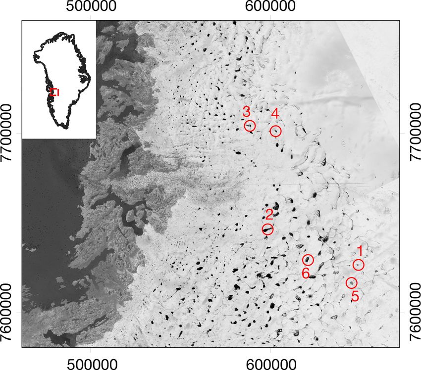
1590                         C. L. Benedek and I. C. Willis: Winter drainage of surface lakes on the Greenland Ice Sheet

   To be certain that a large sudden increase in mean
backscatter is an expression of a change in a particular lake,
rather than an artefact of the sensing process, an anoma-
lous increase in lake backscatter is identified by compar-
ing the mean backscatter change of each lake to that for
all the other lakes in the scene in the same consecutive im-
age pair. For a selection of lakes, the backscatter frequency
distributions were examined and shown to be close to nor-
mally distributed, and thus lake medians and means were
close in value. For each consecutive image pair, the z score
of backscatter change for each lake is calculated relative to
the backscatter change of all lakes within the study site, and
a threshold of +1.5 is used to isolate those lakes that experi-    Figure 2. This figure illustrates the filtering criteria for identifying
ence a greater-than-average increase in backscatter between        drained lakes. (A) Anomalous sustained step change but one that is
images.                                                            not sustained. (B) Anomalous increase but with insufficient history
                                                                   to determine if the change was an adjustment from a previous dip or
   To be sure that a large, anomalous and sudden increase in
                                                                   step increase from a previous low. (C) Anomalous sustained change
backscatter was sustained rather than just an isolated occur-
                                                                   but with a prior dip such that this change was a return to prior val-
rence, filters were employed to check for reversal in the sub-     ues rather than a sustained change. (D) Anomalous change without
sequent three images, where those images occurred within           sufficient information to confirm a sustained change. Lake 2 shows
48 d of the last of the original pair. In each time step, lakes    anomalous, sudden and sustained backscatter change depicting lake
were removed from consideration if the reversed backscatter        drainage. All the time series shown are results from actual lakes in
change was greater than 25 % of the magnitude of the orig-         the 2014/15 season. Bold line segments are the transitions that met
inal anomalous increase (see A in Fig. 2). Time series were        the z-score threshold.
also checked for a dip in backscatter prior to the large rise
(see C in Fig. 2). In the instances where the magnitude of the
dip was greater than 25 % of the magnitude of the sudden in-       each lake was established using a mask based on an NDWIice
crease, that lake was removed from consideration as a drain-       threshold of 0.25. The reflectance values of all pixels imme-
ing lake. The aim of this processing was to identify lakes that    diately exterior (30 m) to this outline were averaged to obtain
showed a sustained backscatter step change increase between        a value for Ad . Rinf was determined per image by selecting
two relatively stable levels (see also B and D in Fig. 2). Given   the darkest pixel (which was always a seawater pixel). For
that there are some large gaps in Sentinel-1 data collection       each lake, the depths of all lake pixels were summed to calcu-
within each relative orbit, specifying that a change event had     late lake volume. Error in the depth calculation follows from
to occur within 12 d and be sustained for up to 48 d reduced       Pope et al. (2016). We take the average of the documented
the number of events compared to those originally detected.        error for the Landsat 8 red band (0.28 m) and that for the
Finally, only lakes greater than 5 pixels in size (0.008 km2 )     panchromatic band (0.63 m) to give an error of 0.46 m. Un-
were considered.                                                   certainty in lake volume follows from this uncertainty in the
                                                                   depth calculation. In line with previous work, we do not de-
2.4    Lake volume                                                 fine errors for lake areas, which instead are fixed according
                                                                   to our threshold NDWIice value of 0.25.
Lake depths were calculated from Landsat 8 imagery us-
ing physical principles based on the Bouguer–Lambert–Beer          2.5   Elevation change from photoclinometry
law as outlined elsewhere (Sneed and Hamilton, 2007; Pope
et al., 2016; Williamson et al., 2018). For the six lakes we       This technique is also known as “shape from shading” and
found that drained in the winter, the latest Landsat 8 images      uses a single surface DEM and a Landsat 8 image to develop
showing the lake prior to freezing over were selected manu-        a relationship between reflectance and slope in a baseline lo-
ally. Lake depth, z, was calculated on a per-pixel basis from      cation to then extrapolate the topography in another. We used
z = [ln(Ad − Rinf ) − ln(Rpix − Rinf )]/g,                  (2)    photoclinometry to reconstruct the topography of the lake
                                                                   surface using winter Landsat 8 images before and after the
where Ad is the lake bottom albedo, Rinf is the reflectance of     drainage event and then produced a differencing image.
a deep-water pixel, Rpix is the reflectance of the pixel being        The ArcticDEM (5 m resolution mosaic) (Porter et al.,
assessed and g is based on calibrated values for Landsat 8         2018) served as the base DEM for area surrounding the lake
(Pope et al., 2016). For this analysis, calculations were per-     and was resampled using bilinear interpolation to match the
formed for both the red and panchromatic bands with the fi-        30 m Landsat 8 resolution. Landsat 8 image pairs were cho-
nal depths taken as the mean of the two results (Pope et al.,      sen to be as close to the timing of each lake drainage as possi-
2016; Williamson et al., 2018). For each band, the outline of      ble both before and after, as well as to be cloud free over the

The Cryosphere, 15, 1587–1606, 2021                                                      https://doi.org/10.5194/tc-15-1587-2021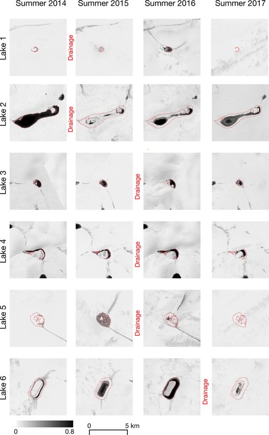
C. L. Benedek and I. C. Willis: Winter drainage of surface lakes on the Greenland Ice Sheet                                  1591

lake, and from the same path and row to reduce any incidence       where between these two, but to account for the different lo-
angle error. All images used were taken when the surface was       cations, DEMs, solar elevations and along-track spacings of
snow covered to ensure that reflectance variation was due to       the sample points between the Iceland and Greenland stud-
the surface slope. The calculations follow the methods out-        ies, we use the larger of the two errors, i.e. 1.61 m. As for
lined by Pope et al. (2013) and were completed for three of        the attenuation-based depth calculations, we do not define er-
the six drained lakes as suitable Landsat 8 image pairs did        rors for lake areas, which are fixed according to our threshold
not exist for the other three.                                     NDWIice value of 0.25.
   For each Landsat 8 image (six in total, two per lake) the
following procedure was adopted. Band 4 was extracted and          2.6    ArcticDEM differencing
used as the basis for calculation. Transects were drawn across
the lake parallel with the solar azimuth at the time of the        We used 2 m time-stamped ArcticDEM strips (Porter et al.,
image. Transects were 10 km in length, to achieve sufficient       2018) from dates prior to and after each drainage but within
coverage of both the lake and ambient area, and were spaced        the winter season to avoid changes due to surface melt. Rele-
250 m apart across the width of the lake. The lake was out-        vant DEMs could only be found for Lake 6 dated 21 Septem-
lined manually based on the Band 4 image, and a 100 m              ber 2016 and 12 March 2017. We calculated the difference
buffer external to the lake boundary was added to ensure that      between these two DEMs in the region of Lake 6 to deter-
the changing lake topography was not included in the pro-          mine changes in surface elevation over this time period and
duction of a baseline relationship between topography and          an independent measure of drained lake volume.
reflectance. Each transect was sampled every 30 m along its           Error in the ArcticDEM depth differential follows from
length for Band 4 reflectance and for elevation in the Arctic-     Noh and Howat (2015). Error in the calculation of the DEM
DEM. Sample lake imagery is shown in Appendix A. The               is approximately 0.2 m, so the height difference error is
surface slope was calculated between each pair of sample           0.28 m.
points outside the buffer region along each transect. A linear
relationship was established between the slope and Band 4          3     Results
reflectance for all sampled points outside the buffered lake
area.                                                              3.1    Winter lake drainage from Sentinel-1 imagery
   For each image processed, the linear slope–reflectance re-
lationship established for non-lake pixels was then applied        We found six lakes that experienced large, anomalous, sud-
to the buffered lake pixels to calculate the slope for each of     den and sustained backscatter increases that we interpret as
the nodes on each transect across the buffered lake area. El-      lake drainage events over the three winter seasons analysed.
evation for each node on each transect across the buffered         Three of these events (lakes 2, 5 and 6) appear clearly in
lake was reconstructed by integrating the slope values, start-     the Sentinel-1 imagery and are supported by optical imagery
ing from the known elevation of the node at the edge of            and photoclinometry evidence with one of them (Lake 6) also
the buffered lake on the north side of the lake and progress-      supported by ArcticDEM differencing. The remaining three
ing to the south side. This resulted in small offset errors on     lakes exhibit a time series of mean backscatter change that is
each transect at the nodes on the south side of the buffered       in line with our expectations of drained lake behaviour, but
lake, where elevations did not match the known elevations          there is insufficient evidence from other datasets to confirm
from the DEM. These offsets were closed by linearly tilt-          drainage.
ing each transect across the buffered lake, adjusting all el-         The locations of the drained lakes are shown in Fig. 1, and
evations accordingly (Appendix A4). Elevation values were          the drainage characteristics are summarized in Table 1. Al-
then interpolated (IDW method) using a 250 m × 30 m grid           though one of the criteria for lake selection was having a
to create a digital elevation model of each lake before and af-    z score of backscatter increase greater than 1.5, results show
ter drainage. These grids were then differenced to calculate       that all six lakes that met all of the criteria had a z score of
the patterns of lake surface elevation change due to winter        backscatter increase greater than 2.0 (Table 1). The size of
lake drainage.                                                     the drained lakes varied widely (between 0.18 and 6.84 km2 )
   Error in the photoclinometry depth calculation is derived       as did the timing of drainage within the winter season, rang-
from Pope et al. (2013), who compared elevations derived us-       ing between early November and late February (Table 1).
ing the photoclinometry method applied to Landsat imagery          During the 2015/16 winter, lakes 3 and 4 towards the north
with airborne lidar elevation data. In areas where the pho-        of the study area and separated by a straight-line distance of
toclinometry assumptions were met (no shading) the median          14.9 km drained within the same 12 d time period (Fig. 1 and
error was just 0.03 m, so the height difference error is 0.04 m.   Table 1).
In areas where the photoclinometry assumptions were not               For each lake, the backscatter changes that signify a
always met (e.g. shaded areas), the median error was 1.44,         drainage are shown in Fig. 3. All lakes generally undergo a
so the height difference error is 1.61 m. We suspect the real      large, anomalous, sudden change from predominantly dark
error for our case on the Greenland Ice Sheet lies some-           (low backscatter) to light (higher backscatter) when com-

https://doi.org/10.5194/tc-15-1587-2021                                                 The Cryosphere, 15, 1587–1606, 2021
1592                             C. L. Benedek and I. C. Willis: Winter drainage of surface lakes on the Greenland Ice Sheet

Table 1. Details of the lake drainage events. Location refers to latitude, longitude (WGS84). The drainage dates are the Sentinel-1 image
dates over which the anomalous change was identified. The 1 dB is the mean change in backscatter (measured in decibels) within the lake
boundary from one image to the next. The z score is the measure of the magnitude of this backscatter change compared to the backscatter
change of other lakes in the study site across the same image pair. Lake area is the size of the lake delineated by the NDWIice -based mask.
Lake volume was calculated as described in Methods.

       Lake           Location     Drainage date           1     z score     Pre-drainage   Pre-drainage       Pre-drainage
                                                          dB                 lake area      mean lake depth    lake volume
       Lake 1   68.70, −47.32      11 to 23 Nov 2014    −4.3         3.5     0.04 km2       0.57 ± 0.46 m      21 212 ± 17 m3
       Lake 2   68.91, −48.52      10 to 22 Jan 2015    −4.4         3.4     6.12 km2       3.26 ± 0.46 m      19 964 800 ± 2817 m3
       Lake 3   69.43, −48.75      5 to 17 Jan 2016     −3.8         2.7     0.43 km2       1.89 ± 0.46 m      809 000 ± 197 m3
       Lake 4   69.40, −48.38      5 to 17 Jan 2016     −2.3         2.6     0.51 km2       2.56 ± 0.46 m      1 318 400 ± 237 m3
       Lake 5   68.62, −47.43      10 to 22 Feb 2016    −3.2         2.8     1.84 km2       0.86 ± 0.46 m      1 593 600 ± 848 m3
       Lake 6   68.75, −48.03      6 to 18 Nov 2016     −9.3         2.2     2.27 km2       1.41 ± 0.46 m      3 188 800 ± 1043 m3

pared to their surroundings. This transition is visually more              3.2   Confirmation of winter lake drainage by optical
obvious for the larger lakes (lakes 1, 2, 5 and 6) and less                      imagery
clear for the smaller lakes (lakes 3 and 4) (Fig. 3) although
the mean backscatter change for Lake 3 is actually slightly                Analysis of Landsat 8 imagery from the summers prior and
greater than that for Lake 5 (Table 1).                                    subsequent to the six inferred winter drainage events sup-
   The mean backscatter time series for each lake is shown                 ports the interpretation that the changing SAR backscatter
in Fig. 4. Each series shows at least two dates of similar                 represents lake drainage. Using the same method described
backscatter values prior to the step change from low to high               above for creating composite NDWIice masks for late sum-
backscatter. Each series maintains its higher backscatter after            mer (from late July and August images), here we create simi-
the initial jump. The backscatter changes of lakes 3 and 4 are             lar NDWIice masks for each summer but using all cloud-free
smaller in decibels than the change that occurs in Lake 6, but             Landsat 8 images between May and August from 2014 to
the z scores signifying how anomalous the jumps are com-                   2017. The purpose of this is to calculate maximum lake areas
pared to those in other lakes are significantly higher in lakes 3          for all lakes, including the six lakes inferred to drain during
and 4 (Table 1).                                                           the winter, in the summers prior and subsequent to the winter
   All other lakes undergo changes in backscatter that are                 lake drainages. Maximum summer water coverages for the
comparable with those in nearby lakes, or they experience                  six winter draining lakes are shown in Table 2. The corre-
large anomalous sudden backscatter changes but ones that                   sponding composite NDWIice images for each summer are
are not sustained. Figure 5 shows the mean backscatter of                  shown in Fig. 6.
Lake 6 over time together with that for the 10 largest lakes in               The maximum lake extents for lakes 1, 2, 5 and 6 appear
its immediate vicinity (within a 20 km × 20 km square, cen-                larger in the summers prior to drainage than after drainage.
tred on Lake 6). The sudden increase in mean backscatter                   This suggests that the winter lake drainages were associated
of Lake 6 is far greater than that for the surrounding lakes.              with fractures/moulins that remained open, allowing the fol-
Lake 6 initially has low backscatter that is comparable with               lowing summers’ meltwater reaching the basin to drain di-
that for some of the surrounding lakes. Optical imagery from               rectly into the ice sheet. These reductions in maximum lake
the end of the previous summer shows Lake 6 and these other                extents contrast with those observed for the many surround-
“low-backscatter lakes” were water filled. Over a single im-               ing lakes, which fill to around the same size in the adja-
age transition (12 d), Lake 6 experiences a backscatter in-                cent summers. Lakes 3 and 4 show little difference in area
crease to levels that are comparable with other surrounding                before and after drainage, but the lakes do change shape
lakes that optical imagery from the end of the previous sum-               (Fig. 6). This suggests that the fractures/moulins associated
mer showed were drained. The lakes surrounding Lake 6 ex-                  with the winter drainage of these lakes closed shut or were
perience much slower backscatter increases over time, which                advected out of the lake basins, allowing the lakes to form
we interpret to be slow freezing of the water in the filled lakes          again in the subsequent summer. Lakes that experience large
or the ice surface in the bottom of the drained lakes. Figure 5            area changes recover their area over time but not necessarily
also illustrates what the backscatter changes look like within             within the first summer following drainage.
the Sentinel-1 imagery. Small changes are observable within
the surrounding lakes, but a much bigger change is seen in
Lake 6.

The Cryosphere, 15, 1587–1606, 2021                                                           https://doi.org/10.5194/tc-15-1587-2021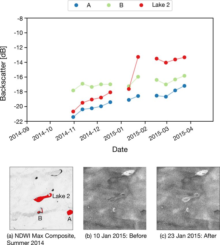
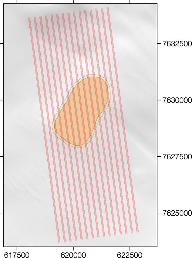
C. L. Benedek and I. C. Willis: Winter drainage of surface lakes on the Greenland Ice Sheet                                         1593

Table 2. Maximum lake area for each summer generated by calculating the maximum NDWIice per pixel from May to August each year.
The lake NDWIice threshold is set at 0.25, and area is calculated based on all pixels in the lake above this value.

                                                                     Lake areas (km2 )
                             Lake         Summer 2014       Summer 2015        Summer 2016    Summer 2017
                             Lake 1       0.0936*           0.0189             0.4734         0 (cloud cover)
                             Lake 2       6.498*            0.936              2.774          3.595
                             Lake 3       0.967             0.934*             1.532          0.698
                             Lake 4       0.699             0.639*             0.658          0.495
                             Lake 5       0.166             2.201*             0.471          0 (cloud cover)
                             Lake 6       1.001             1.987              2.757*         0.614

                           * Indicates pre-drainage area.

3.3   Confirmation of lake drainage by photoclinometry                     the ArcticDEM strips is 3.66 ± 0.28 m and that from the pho-
      and ArcticDEM differencing                                           toclinometry is 4.04 ± 1.61 m.

Finally, we used two additional techniques to support the                  4     Discussion
conclusion that the observed changes in Sentinel-1 backscat-
ter are lake drainages. First, we used photoclinometry based               We have developed a novel algorithm for analysis of
on the 5 m ArcticDEM mosaic and Landsat 8 imagery be-                      Sentinel-1 SAR imagery and used it to identify six winter
fore and after the winter drainage events (see Methods)                    lake drainage events on the GrIS, the first such events to be
to calculate surface elevation changes across three of the                 reported in full. Because SAR backscatter is often difficult to
lakes (Fig. 7). Landsat 8 images suggest a smooth flat sur-                interpret (White et al., 2015) we have validated our technique
face to each lake prior to drainage and a rough topog-                     by examining Landsat 8 optical imagery from the previous
raphy following drainage, suggesting the caving-in of a                    and subsequent summers. Changes in lake area and volume
frozen, snow-covered lake surface during drainage. Mean                    as well as topographic changes calculated using photocli-
elevation changes calculated from photoclinometry using                    nometry support the inference that these large, anomalous,
these images are 7.25 ± 1.61 m for Lake 2, 1.21 ± 1.61 m                   sudden and sustained backscatter increases are lake drainage
for Lake 5 and 3.38 ± 1.61 m for Lake 6. These depths are                  events. We have also been able to validate the winter drainage
greater than those calculated based on the last available op-              of one of these lakes by differencing available ArcticDEM
tical image, seen in Table 1, but are internally consistent in             strips.
their rank from smallest to largest. Possible reasons for the
discrepancy between attenuation-based depth estimates and                  4.1    Identifying lake drainage events
photoclinometry-based collapse depths are addressed in the
Discussion.                                                                Identification of winter lake drainage events using Sentinel-1
   Second, we examined differences in ArcticDEM strips                     data required multiple steps to isolate drainage events from
from dates during the winter on either side of the Lake 6                  other changes in backscatter. The drainage events identi-
drainage event. Elevation change between time-stamped Arc-                 fied occurred in lakes of various sizes and in various lo-
ticDEM strips from 21 September 2016 and 12 March 2017                     cations. If lakes are identified as anomalous based on their
is shown in Fig. 8. Elevation change is greater within the lake            z score with no additional filtration performed to confirm
area than surrounding it. Delineating lakes based on optically             sustained change, the three seasons analysed would result in
visible water means that the lake outlines may omit possi-                 188, 160 and 221 anomalous lakes for the 2014/15, 2015/16
ble subsurface water obscured by an ice lid. It appears from               and 2016/17 winter seasons, respectively. For each of these
the Sentinel-1 imagery (Figs. 5 and 3) that Lake 6 contains                years, retaining only lakes that met the 1.5 z-score thresh-
a floating ice island obscuring water beneath. The mean of                 old and demonstrated no reversal of trend in the first time
the differenced ArcticDEM within the NDWIice -based mask                   step would result in 75, 60 and 85 lakes, respectively. Re-
outline of Lake 6 is 2.17 ± 0.28 m. Note this compares with                versal was considered to be any change greater than 25 % of
the mean depth derived from the optically based depth calcu-               the magnitude of the anomalous transition occurring either
lations of 1.41 ± 0.46 m and that from the photoclinometry                 in the previous time step or in the following three time steps.
method of 3.38 ± 1.61 m (Fig. 7). If the entire closed volume              Raising this threshold to 30 % would result in 4 anomalous
of Lake 6 is considered and the data for the entire area are               lakes for each season. Raising the same threshold to 40 %
included in the analysis, the mean elevation difference from               would result in 10, 7 and 10 lakes for the three seasons, re-

https://doi.org/10.5194/tc-15-1587-2021                                                         The Cryosphere, 15, 1587–1606, 2021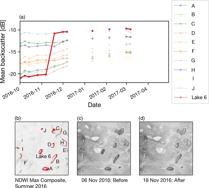
1594                            C. L. Benedek and I. C. Willis: Winter drainage of surface lakes on the Greenland Ice Sheet

                                                                        Figure 4. Backscatter time series for the lakes with identified
                                                                        drainage events. Connecting lines are only included when the time
                                                                        between images is 12 d or less. Each series represents one lake, and
                                                                        each point represents the mean backscatter of all of the lake’s pixels
                                                                        in a particular Sentinel-1 image. Bold lines indicate the transition
                                                                        determined to be the drainage event.

Figure 3. Sentinel-1 backscatter for each lake immediately before       false negatives) than to have found drainage events that were
and after drainage. Before and after drainage dates are listed in Ta-   not real (incorporated false positives).
ble 1. Note the lakes before drainage have a lower backscatter that
changes to a higher backscatter across the image pair. Red outlines     4.2   Optical lake mask
indicate the delineated lake boundary based on the NDWIice thresh-
old.                                                                    As lake delineation using Sentinel-1 backscatter alone is not
                                                                        trivial (Miles et al., 2017; Wangchuk et al., 2019), all change
                                                                        tracking in this study is based on pixels within lake out-
                                                                        lines generated from Landsat 8 optical imagery. However,
spectively. Raising it again to 50 % would result in 25, 19 and         in comparing the optically generated masks to the Sentinel-
21 lakes for the three seasons.                                         1 backscatter images, the two are often different, typically
   Extending the requirement for stability by requiring more            with the SAR images showing larger lake areas than those
consecutive images without reversal would be difficult in               seen in the optical data. This discrepancy may be due to wa-
most years due to the limited image acquisition over this site.         ter depths that are insufficient to meet the NDWIice thresh-
Overall the filtration proved not to be overly sensitive to the         old set or to shallow subsurface water below a snow or ice
z-score threshold, as all drained lakes had z scores over 2             lid. This is most apparent in Lake 6 (Figs. 5 and 6), where
even though the threshold was set to 1.5. The criteria used to          a low-NDWIice island appears in the centre of the lake, but
determine lake drainage events is thought to be conservative            HV backscatter measurements, which are sensitive to volu-
and is more likely to have missed drainage events (included             metric scattering, remain low in this portion and both pho-

The Cryosphere, 15, 1587–1606, 2021                                                          https://doi.org/10.5194/tc-15-1587-2021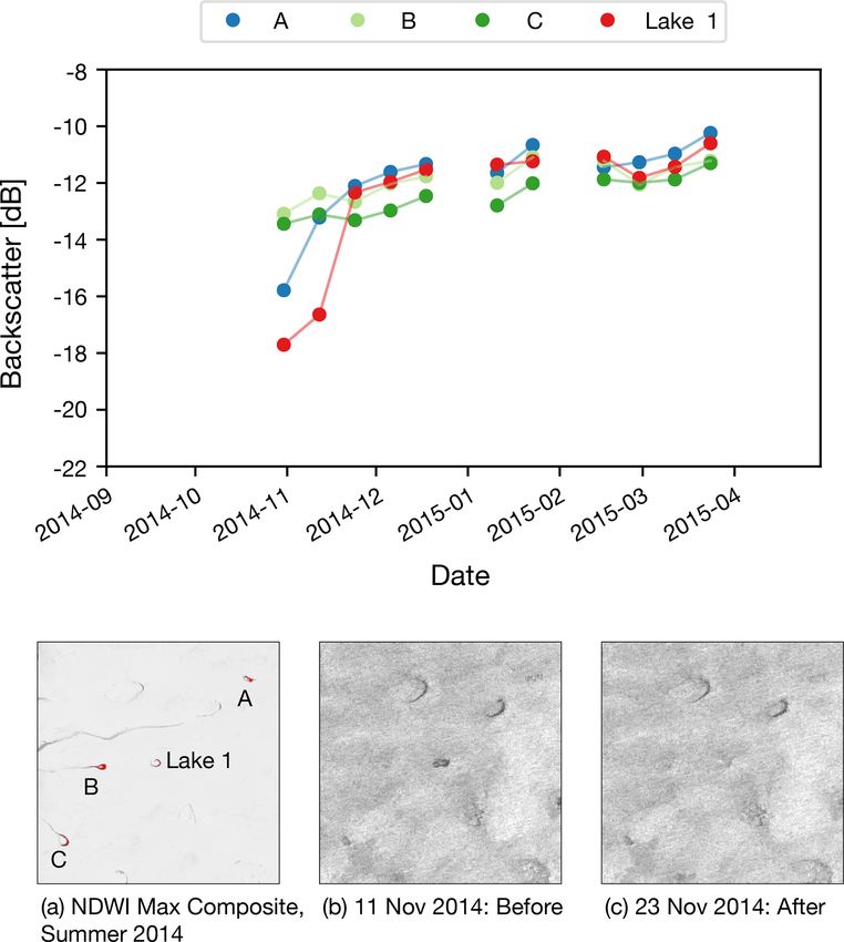
C. L. Benedek and I. C. Willis: Winter drainage of surface lakes on the Greenland Ice Sheet                                      1595

Figure 5. (a) Sentinel-1 backscatter time series for the largest 10
lakes within 10 km of Lake 6. Connective lines are omitted from
the time series graph when the time between images is greater than
12 d. Image (b) is a composite maximum NDWIice image for late
summer 2016, prior to lake drainage showing the lakes included
in the graph above. Images (c) and (d) are Sentinel-1 backscatter
images for 6 and 18 November 2016 across which the drainage of
Lake 6 is observed. While the backscatter of the surrounding lakes
undergoes a small gradual increase over time, the backscatter in-
crease of Lake 6 is much greater than that seen in the other lakes.

toclinometry and ArcticDEM changes show a caving-in of
ice in this area (Figs. 5 and 8). Beginning with the NDWIice
mask also results in the splitting of some lakes into multiple        Figure 6. NDWIice for each identified drained lake at the peak of
                                                                      each summer within the study. Note that most lakes take more than
disconnected water bodies where parts of the lake are be-
                                                                      a single summer season to recover from their winter drainage.
low the threshold. Therefore, some larger lakes may be fil-
tered out of the study as they appear to be a collection of
smaller lakes, and some backscatter tracking is only occur-           summer, although the lower backscatter in this area seems to
ring on partial lakes, where only deeper portions with higher         indicate shallow subsurface water.
NDWIice values are included in the lake delineation. Other
surface changes, such as the drainage of a subglacial lake,           4.3   Sentinel-1 backscatter
could result in SAR backscatter changes as well. The aim of
restricting the analysis to lakes that are optically identifiable     While Sentinel-1 backscatter allows for the tracking of lakes
in the summer is to reduce the likelihood that the changes            that are obscured by cloud cover and darkness, it is also
identified in this study are due to such events.                      limited in what it can observe. The penetration depth of C-
   We have used masks created from just a few summer                  band radar producing backscatter varies based on the phys-
images to reduce the likelihood of incorporating lakes that           ical properties of the medium through which it passes, es-
drained in the summer into our wintertime lake tracking al-           pecially moisture content, but reaches a maximum of a few
gorithm. Creating lake masks using a longer time span of              metres of depth (Rignot et al., 2001). However, it is also pos-
images might allow for more complete lake boundaries to be            sible that winter lakes exist below this depth and are not de-
included. By including more summer images, these masks                tected. This penetration depth is also likely to be insufficient
might account for areas of water that are only occasionally           to reach the buried firn aquifers identified in the Greenland
seen at the surface but are more often under snow or ice, thus        Ice Sheet (Forster et al., 2014; Koenig et al., 2014).
especially those at higher elevations. Lake 1, for example,              In our study, three images showed large, scene-wide de-
often appears below the 0.25 NDWIice threshold due to the             partures from typical backscatter values and were omitted
absence of cloud-free and unfrozen images within a given              from further analysis (dated 3 February 2015, 10 April 2016

https://doi.org/10.5194/tc-15-1587-2021                                                     The Cryosphere, 15, 1587–1606, 2021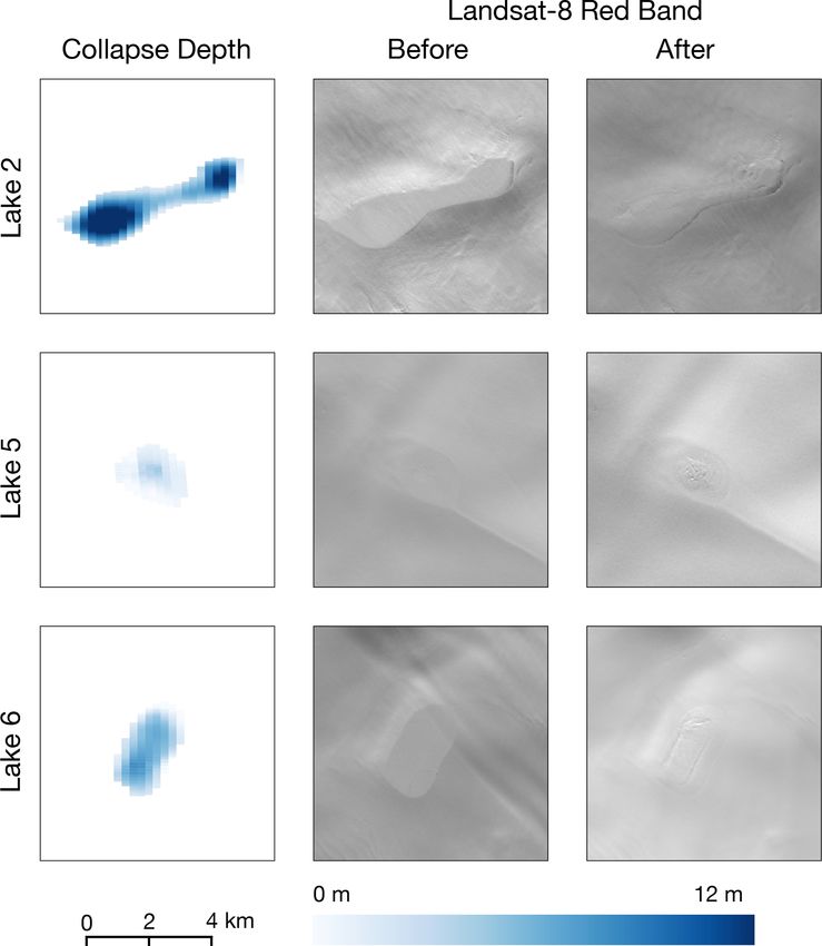
1596                            C. L. Benedek and I. C. Willis: Winter drainage of surface lakes on the Greenland Ice Sheet

                                                                        tween 6 and 18 November 2016, a 12 d gap in sensing and
                                                                        the dates between which Lake 6 drained. If additional orbits
                                                                        had been included in this analysis, the gap could have been
                                                                        reduced to 10 d but no further.

                                                                        4.4   Drainage water volume

                                                                        Sentinel-1 backscatter alone does not allow for the calcula-
                                                                        tion of water volumes and therefore water volume changes.
                                                                        Available optical satellite data can be used to estimate wa-
                                                                        ter volume, but the optical measurements are limited in their
                                                                        capability to calculate accurately the drained volume. In this
                                                                        study, physically based depth estimates are made on a per-
                                                                        pixel basis for each lake using the last available image in
                                                                        the summer before the lake is covered by a frozen lid (Ta-
                                                                        ble 1). However, there are several sources of error associ-
                                                                        ated with these measurements. First, the measurements have
                                                                        been shown to underestimate the depth of deep water (Pope
                                                                        et al., 2016; Williamson et al., 2018). Second, the measure-
                                                                        ments made months prior to the drainage events and the lake
                                                                        volumes derived from them could be impacted by additional
                                                                        melt filling the lake or freezing of water prior to the drainage
Figure 7. Elevation difference results of the photoclinometry anal-
ysis beside the before and after images (Landsat 8 red band, B4)        event. Third, the lake boundary is set using an NDWIice
to illustrate the visible physical changes to the lake lid before and   threshold of 0.25, which may underestimate the full extent
after drainage. The first column of images shows the vertical eleva-    of the lake area. Fourth, the calculation assumes all the lake
tion drop of each pixel calculated by interpolating and differencing    water from the previous autumn drains. There is no reliable
the pre- and post-drainage topography.                                  method of using optical data to measure whether any water
                                                                        remains at the start of the subsequent melt season. Images
                                                                        showing the first water visible in the spring after drainage
                                                                        could be showing water remaining in the lake or water trans-
                                                                        ported into the basin from higher elevations that year. Often
                                                                        cloud-free images are not available until well into the melt
                                                                        season and thus cannot reliably be used as a lower bound in
                                                                        a calculation of water volume difference from the previous
                                                                        autumn.
                                                                           Photoclinometry results show, for each lake, a topograph-
                                                                        ical change in the surface shape between the pre- and post-
Figure 8. Elevation difference results of the ArcticDEM analysis to     drainage images indicating an elevation drop. However, the
confirm the changes observed in the Sentinel-1 imagery and photo-       depth of caving is greater than the deepest water depth deter-
clinometry analyses.                                                    mined from the light-attenuation-based method using optical
                                                                        imagery from the previous autumn. The depth estimation dif-
                                                                        ferences may be the result of a combination of factors. As
and 16 May 2016). If it were known what caused this phe-                mentioned above, the attenuation-based algorithm is known
nomenon, then perhaps the images could be corrected and                 to underestimate lake depths as the depths increase beyond a
used.                                                                   certain threshold (Pope et al., 2016; Williamson et al., 2018).
   Sentinel-1 is also limited in its temporal frequency of              Furthermore, photoclinometry-based depths may overesti-
available imagery for the same site. While the repeat pass              mate collapse depths due to topography changes between the
time of Sentinel-1 is at best 6 d when both satellites are in-          date of the DEM and the date of the optical imagery used
cluded (only available since late 2016), it is advisable to use         to create the shape–shading relationship. Finally, shadows
imagery from the same relative orbit for greater consistency            within the lake basin that do not appear in parts of the im-
from image to image, and not all images within each path are            age surrounding the lake may also introduce errors into the
acquired. A shorter repeat pass could help more accurately              calculation of shape from shading within the basin.
assess the rate of backscatter change and thus gain a bet-                 While the depth estimation using this photoclinometry
ter understanding of the speed and timing of these drainage             may be inaccurate in places for the reasons outlined above,
events. For example, no image in Relative Orbit 17 exists be-           the technique confirms that a change in surface topography

The Cryosphere, 15, 1587–1606, 2021                                                        https://doi.org/10.5194/tc-15-1587-2021
C. L. Benedek and I. C. Willis: Winter drainage of surface lakes on the Greenland Ice Sheet 1597
occurred. Photoclinometry is potentially a useful method for Chudley et al., 2020). There is no obvious correlation be-
detecting surface or shallow subsurface lake drainages on ice tween ice speed patterns and the location of winter lake
sheets and ice shelves. The optical data support the asser- drainage events, suggesting that patterns of ice flow are not
tion that the changes in winter SAR backscatter observed are necessarily a trigger for drainage. Our sample size is small,
caused by lake drainage events. The larger lakes in the study, however, and more evidence is needed to examine further
lakes 2, 5 and 6, all show a significant reduction in lake area the possibility. In this study, most of the lake drainages occur
in the summer following the winter drainage compared to in isolation – with the exception of the drainages of lakes 3
the previous summer with more than a single summer season and 4, which occur in the same 12 d period. These lakes are
needed to regain pre-drainage lake area (Fig. 7). This may be separated by a linear distance of 14.9 km. These concurrent
due to the opening of a fracture that continues to allow water drainage events may be related, with one drainage triggering
to drain through the lake bed for some time, similar to that the other by creating localized ice acceleration transferred via
found by Chudley et al. (2019). Lake 1 shows a similar slow stress gradients (Christoffersen et al., 2018). Alternatively,
re-filling over time, but the effect is less clear in lakes 3 and they may indicate a larger-scale ice movement that triggered
4. both events simultaneously.
Compared to lakes 1, 2, 5 and 6, lakes 3 and 4 did re-fill to
their former size in the summer following drainage (Fig. 6).
While these two lakes did show a large, anomalous, sudden 5 Conclusions
and sustained backscatter increase suggesting winter lake
We have developed an automated method for identifying
drainage according to our criteria, they were small in area and
large, anomalous, sudden and sustained backscatter changes
the subsequent filling makes it less clear that drainage events
in Sentinel-1 SAR imagery, which we apply to images col-
actually occurred. These lakes also lack the additional sup-
lected between October and May spanning three winter sea-
port of photoclinometry or ArcticDEM differencing to con-
sons. We find four winter lake drainage events across a study
firm that the lakes definitively drained. The SAR backscatter
site containing approximately 300 supraglacial lakes that are
changes suggest that the lakes did drain, and if this is the
supported by optical data and two other possible drainage
case, the available optical data suggest that any fracture cre-
events that meet our backscatter change criteria but lack the
ated during drainage may have been subsequently squeezed
optical data support to unequivocally confirm drainage.
shut or advected out of the small lake basin allowing the lakes
The optical imagery from before the winter seasons is
to fill again the following summer.
used to provide estimates of lake volumes associated with
The drainage of Lake 6 is further confirmed by the anal-
the drainages. While the events are rare, they provide conclu-
ysis of the ArcticDEM differential (Fig. 8), which shows a
sive evidence for the first time that lake drainages over win-
collapse across the entire lake area, including the central area
ter occur. They are likely triggered simply by crevasse open-
that did not appear as deep water in any preceding-summer
ing across the lake due to high surface strain rates associated
Landsat 8 images. The collapse is greatest at the centre and
with background winter ice movement. This shows that rapid
decreases towards the edges of the lake boundary. The mag-
lake drainage events do not have to be triggered during lake
nitude of the collapse as measured by the DEM differential
water filling, as has been observed previously for summer
is similar to that measured by the photoclinometry method.
events. A full picture of the hydrology of the Greenland Ice
Furthermore, the nearby lakes show no significant elevation
Sheet requires observation of surface water on a multi-year
change across the same period.
and multi-season basis. Identification of the drainage events
was achieved by developing a time-series-filtering algorithm
4.5 Causes and implications of lake drainage
that may be adapted to identify other hydrological phenom-
ena such as the onset of melt or the rate of filling or freezing
The causes of lake drainage events have been studied exten-
of surface or shallow subsurface water bodies on ice sheets
sively (Williamson et al., 2018; Christoffersen et al., 2018).
and ice shelves. The algorithm is based on a set of thresholds
However the observation of isolated winter lake drainages
that were set conservatively to capture only the most obvi-
points to the possibility that drainages can occur without in-
ous incidences of large, anomalous, sudden and sustained
creases to lake volume that actively cause hydrofracture or
backscatter changes, and therefore our study is more likely
connection to a nearby moulin to trigger sliding or uplift
to have underestimated rather than overestimated the num-
and passively open a crack. Instead, it shows that ice dy-
ber of winter lake drainages (included false negatives rather
namics unrelated to surface hydrology can trigger drainage.
than false positives). Further work is required to examine
The evidence available in this study is insufficient to iden-
whether winter lake drainage occurs in other parts of the ice
tify conclusively the cause of these winter lake drainages.
sheet and in other years, what the triggering mechanisms are,
Appendix Fig. B1 shows the locations of the winter lake
how basal hydrology and biogeochemistry are affected, and
drainage events compared to ice speeds derived from MEa-
whether winter lake drainage will become more prevalent un-
SUREs data (Howat, 2017) for the winter periods contain-
der future climate warming scenarios.
ing each drainage event (calculation methods developed by
https://doi.org/10.5194/tc-15-1587-2021 The Cryosphere, 15, 1587–1606, 20211598 C. L. Benedek and I. C. Willis: Winter drainage of surface lakes on the Greenland Ice Sheet
Appendix A: Photoclinometry process A3 Lake sampling
A1 Images Figure A2 shows the set-up for the photoclinometry portion
of the study. The lake was manually outlined and buffered,
and transects were spaced every 250 m and sampled every
Table A1. Landsat 8 image IDs used for photoclinometry. 30m along the transect for each 10 km long transect.
Lake Landsat 8 Scene
Lake 2 Before LC08_008012_20141101
Lake 2 After LC08_008012_20150221
Lake 5 Before LC08_008011_20151104
Lake 5 After LC08_008011_20160428
Lake 6 Before LC08_009011_20161028
Lake 6 After LC08_009011_20170217
A2 Slope vs. reflectance
Figure A1 shows the correlation of slope with reflectance for
the non-lake areas of each of the Landsat 8 images used in
the photoclinometry section of this study. For each image, a
new relationship was established and used to infer the slope
of the lake area within that image.
Figure A2. Lake 6 transects for photoclinometry calculations for
the image on 28 October 2016 prior to drainage (red), lake extent
(orange) and buffer (yellow). For a description of how these features
are used in the photoclinometry calculations, see Methods.
A4 Photoclinometry point sampling
Figure A3 shows the correction of a transect across the lake.
Transect A in the graph was the original transect calculated
following the photoclinometry process. Transect B is the re-
sult of correction by calculating the elevation difference be-
tween the end of the lake transect and the elevation at that
lake edge in the ArcticDEM and then distributing that eleva-
tion difference evenly across the lake transect.
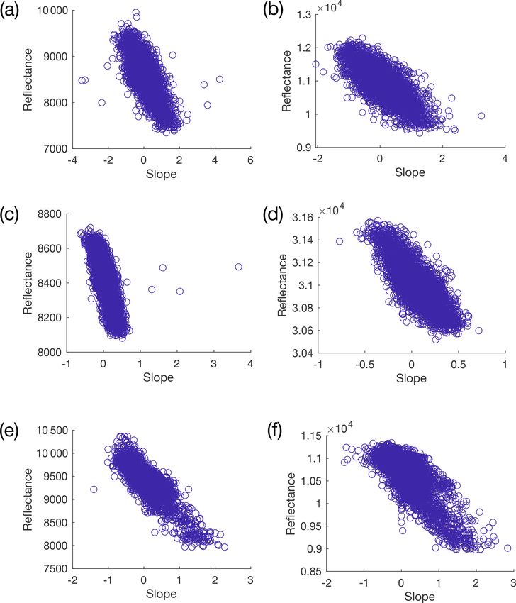
Figure A1. Plots of slope vs. Landsat 8 red-band reflectance for
areas outside of the lake and buffer zone for each of the Landsat 8
images analysed for the photoclinometry portion of this study. The
plots are laid out as follows: (a) Lake 2 Before, (b) Lake 2 After, (c) Figure A3. An example Lake 6 transect pair for photoclinometry
Lake 5 Before, (d) Lake 5 After, (e) Lake 6 Before and (f) Lake 6 calculations before (red) and after (blue) correction.
After.
The Cryosphere, 15, 1587–1606, 2021 https://doi.org/10.5194/tc-15-1587-2021C. L. Benedek and I. C. Willis: Winter drainage of surface lakes on the Greenland Ice Sheet 1599
Appendix B Appendix C
Figure B1 presents pixel-by-pixel ice speeds based on MEa- This figure shows the behaviour of lakes surrounding the
SUREs velocity data (Howat, 2017) for the winters surround- identified drained lakes for the summers included in this
ing each of the drainage events. study. The images shown are peak values of the NDWIice
for each pixel, creating a maximum composite image. Red
shading covers the extent of the lake mask for each year.
Figure B1. Ice speeds for the winter quarter proximate to each of
the lake drainages.
Figure C1. Composite maximum NDWIice images for each sum-
mer. Each pixel shows the highest NDWIice reached for that pixel
for the season. The red outlines show the lake outlines as delineated
by a threshold exceeding 0.25 in the maximum NDWIice composite
for the pre-drainage summer. Red boxes identify each anomalous
lake.
https://doi.org/10.5194/tc-15-1587-2021 The Cryosphere, 15, 1587–1606, 20211600 C. L. Benedek and I. C. Willis: Winter drainage of surface lakes on the Greenland Ice Sheet
Appendix D
The figures in this appendix show the backscatter time se-
ries for the lakes proximate to each of the identified drainage
events. These are the equivalent of Fig. 5 for all the lakes
apart from Lake 6, which is shown in the body of the paper.
For each figure, the top panels shows the backscatter time se-
ries. In the bottom row, panel (a) shows the lakes captured by
the NDWIice mask, panel (b) shows the backscatter prior to
the drainage event and panel (c) shows the backscatter after
the drainage event.
Figure D2. Lake 2 surrounding lakes.
Figure D1. Lake 1 surrounding lakes.
Figure D3. Lake 3 surrounding lakes.
The Cryosphere, 15, 1587–1606, 2021 https://doi.org/10.5194/tc-15-1587-2021You can also read