Improving sub-canopy snow depth mapping with unmanned aerial vehicles: lidar versus structure-from-motion techniques
←
→
Page content transcription
If your browser does not render page correctly, please read the page content below
The Cryosphere, 14, 1919–1935, 2020
https://doi.org/10.5194/tc-14-1919-2020
© Author(s) 2020. This work is distributed under
the Creative Commons Attribution 4.0 License.

Improving sub-canopy snow depth mapping with unmanned aerial
vehicles: lidar versus structure-from-motion techniques
Phillip Harder1 , John W. Pomeroy1 , and Warren D. Helgason1,2
1 Centre
       for Hydrology, University of Saskatchewan, Saskatoon, Saskatchewan, Canada
2 Department of Civil, Geological, and Environmental Engineering, University of Saskatchewan,
Saskatoon, Saskatchewan, Canada

Correspondence: Phillip Harder (phillip.harder@usask.ca)

Received: 23 November 2019 – Discussion started: 16 December 2019
Revised: 29 April 2020 – Accepted: 5 May 2020 – Published: 15 June 2020

Abstract. Vegetation has a tremendous influence on snow         quantify the many multiscale snow processes defining snow-
processes and snowpack dynamics, yet remote sensing tech-       pack dynamics in mountain and prairie environments.
niques to resolve the spatial variability of sub-canopy snow
depth are not always available and are difficult from space-
based platforms. Unmanned aerial vehicles (UAVs) have had
recent widespread application to capture high-resolution in-    1   Introduction
formation on snow processes and are herein applied to the
sub-canopy snow depth challenge. Previous demonstrations        Snow accumulation and melt are critical parts of the hydro-
of snow depth mapping with UAV structure from motion            logical cycle in cold regions (King et al., 2008). To under-
(SfM) and airborne lidar have focussed on non-vegetated         stand these processes, there needs to be robust and accurate
surfaces or reported large errors in the presence of vegeta-    observation methodologies to measure the depth and den-
tion. In contrast, UAV-lidar systems have high-density point    sity of a snowpack and its change across all aspects of the
clouds and measure returns from a wide range of scan angles,    landscape. Unfortunately, satellite remote sensing methods
increasing the likelihood of successfully sensing the sub-      struggle to quantify the spatial distribution of snow at a high
canopy snow depth. The effectiveness of UAV lidar and UAV       enough resolution and accuracy to account for the fine-scale
SfM in mapping snow depth in both open and forested terrain     interactions between snow and vegetation (Nolin, 2010). Re-
was tested in a 2019 field campaign at the Canadian Rockies     mote sensing conceptually promises the capability to gather
Hydrological Observatory, Alberta, and at Canadian prairie      this type of data at the spatial scales and extents needed, but
sites near Saskatoon, Saskatchewan, Canada. Only UAV li-        the main challenge for snow observations across a heteroge-
dar could successfully measure the sub-canopy snow surface      neous landscape is that exposed vegetation and forests ob-
with reliable sub-canopy point coverage and consistent er-      scure the underlying snow surface (Bhardwaj et al., 2016;
ror metrics (root mean square error (RMSE)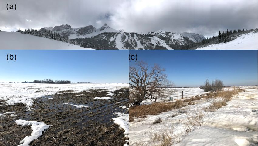
1920                          P. Harder et al.: Improving sub-canopy snow depth mapping with unmanned aerial vehicles

hydrology, test processes, examine the spatial scaling of pro-      wind conditions, or solar illumination. A clear benefit of li-
cess interactions (Clark et al., 2011; Deems et al., 2006; Tru-     dar is that multiple returns per pulse can be observed with
jillo et al., 2007), and to initialise and/or validate model pre-   returns possible from within the canopy and from the sub-
dictions (Hedrick et al., 2018). Snow depth, the focus of this      canopy ground or snow surface. In contrast UAV SfM uses
paper, is not the variable of ultimate interest for hydrology.      a passive RGB sensor where data quality is not actively con-
Rather, snow water equivalent (SWE) is used for snow hy-            trolled. This results in variable image quality because incon-
drology applications (Pomeroy and Gray, 1995). Fully cog-           sistent solar illumination influences image exposure, wind
nisant of this, the focus here is on snow depth, as it is well      gusts influence platform stability leading to blurry images
documented that snow depth varies much more than density            and inconsistent overlap, and surface heterogeneity means
(Pomeroy and Gray, 1995; Shook and Gray, 1996; Jonas et             that some areas of the domain will have more key points –
al., 2009; López-Moreno et al., 2013); therefore, improving         points automatically detected and matched in multiple im-
the accuracy of snow depth observations in a drainage basin         ages (Westoby et al., 2012) – leading to variability in the
is critical to improving the estimation of SWE at and within        quality of the SfM solution (Bühler et al., 2016; Harder et
basin scales.                                                       al., 2016; Meyer and Skiles, 2019). So while SfM can pro-
    Snow depth and SWE observations are traditionally col-          vide similar quality error metrics in open areas, the quality
lected through in situ observations (Goodison et al., 1987;         will vary between flights as conditions change, whereas li-
Helms et al., 2008; Kinar and Pomeroy, 2015a; Sturm,                dar will be more consistent. Reported snow depth accuracy
2015). In situ approaches, such as snow surveying, rely             in open environments, expressed as root mean square errors
on manual sampling of snow depths and densities to get              (RMSEs), varies from 0.08 to 0.60 m for airborne lidar (Cur-
SWE. When conducted along landscape-stratified transects,           rier et al., 2019; DeBeer and Pomeroy, 2010; Harpold et al.,
the landscape-scale SWE can be estimated (Pomeroy and               2014; Mazzotti et al., 2019; Painter et al., 2016; Tinkham et
Gray, 1995; Steppuhn and Dyck, 1974). The challenge for             al., 2014), 0.17 to 0.30 m for airborne SfM (Bühler et al.,
snow survey observations is that they are prone to observer         2015; Meyer and Skiles, 2019; Nolan et al., 2015), and 0.02
bias, are labour-intensive and time-consuming, and are of-          to 0.30 m for UAV SfM (Harder et al., 2016; Vander Jagt
ten unable to sample all aspects of a landscape such as             et al., 2015; De Michele et al., 2016). A notable challenge
avalanche zones (Kinar and Pomeroy, 2015a). Nonetheless,            is that the presence of exposed vegetation, especially dense
snow surveying is a proven approach to quantify SWE and             forest, confounds SfM solutions and obscures airborne-lidar
has been operationalised across many regions. The practice          bare-surface extractions which are needed for fine-scale dif-
has historical precedence and has created many long-term            ferencing of DEMs to evaluate snow depths or snow depth
records which are a valuable data source (Goodison et al.,          changes (Bhardwaj et al., 2016; Deems et al., 2013; Harpold
1987; Helms et al., 2008). Other point observations, such           et al., 2014). Terrestrial laser scanning (TLS) is another ap-
as snow pillows (Coles et al., 1985), acoustic sensors (Ki-         proach for observing high-resolution snow depth data which
nar and Pomeroy, 2009, 2015b), and passive gamma sen-               has been used to develop an understanding of snow depth
sors (Smith et al., 2017), are valuable automated data sources      distributions and for validating other snow depth observation
but are spatially limited in extent and can often suffer from       methods (Currier et al., 2019; Egli et al., 2012; Grünewald
location/elevation bias – as demonstrated by the SNOTEL             et al., 2010; Mott et al., 2011). However, TLS has important
network in the western United States (Molotch and Bales,            limitations that restrict further landscape-scale understand-
2006). In particular, measurements of snow in forest clear-         ing of snow processes in forested areas as it is limited by the
ings will have relatively more snow than under the adjacent         site-specific viewshed and viewing geometry (Deems et al.,
canopy (Pomeroy and Gray, 1995), and so they may not be             2013) and occlusion by forest canopies and low vegetation,
suitable for snow hydrology calculations or model valida-           which decreases point cloud density away from forest edges
tions in forested regions even though they are often used for       (Currier et al., 2019). TLS remains an excellent technique for
just such purposes. Other techniques need to be developed to        detailed examination of the forest-edge snow environment.
capture the small-scale spatial variability of snow–vegetation         Most applications of remote sensing for observing snow
interactions to advance our process understandings and vali-        processes have focussed on open environments. However,
date the next generation of distributed snow models.                vegetated portions of those same environments can play a
    Remote sensing approaches have shown promise in eval-           large role in landscape-scale snow hydrology. For example,
uating snow depth in open areas. Airborne-lidar and UAV             wetland vegetation accumulates deep snowdrifts and so has
structure-from-motion (SfM) approaches have been proven             an exaggerated influence on snow accumulation processes
to provide snow depth mapping abilities when differenc-             in prairie environments (Fang and Pomeroy, 2009). Simi-
ing snow-covered (hereafter snow) and snow-free (hereafter          larly, forests constitute large fractions of the mountain do-
ground) digital elevation models (DEMs). Lidar, an active           main (Callaghan et al., 2011; Troendle, 1983) and have very
sensor, emits a pulse of light, and the detection of the re-        different snow processes than those found in open environ-
flected pulse results in a point cloud of a scene with a con-       ments (Pomeroy et al., 2002). Snow–vegetation interactions
sistent quality point cloud regardless of flight characteristics,   are complex (Currier and Lundquist, 2018; Gelfan et al.,

The Cryosphere, 14, 1919–1935, 2020                                                    https://doi.org/10.5194/tc-14-1919-2020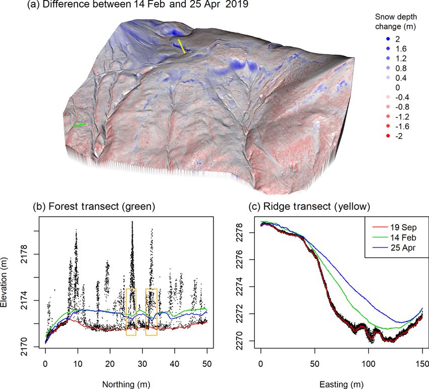
P. Harder et al.: Improving sub-canopy snow depth mapping with unmanned aerial vehicles 1921
2004; Hedstrom and Pomeroy, 1998; Harder et al., 2018; was developed as an alpine ski resort in the 1960s but is
Mazzotti et al., 2019; Musselman et al., 2008; Parviainen and currently a limited-use ski operation without snowmaking,
Pomeroy, 2000; Pomeroy et al., 2001; Zheng et al., 2016) and and some open ski runs remain through some of the slopes
involve both snow interception by the canopy and wind redis- of interest. Strong winds result in substantial redistribution
tribution to forest edges. In dense forests, vegetation leads to of snow by blowing snow in this environment (Aksamit and
the interception and subsequent sublimation of snow, result- Pomeroy, 2018)
ing in an overall decrease in accumulation (Hedstrom and Two study areas in the Canadian Prairies were examined
Pomeroy, 1998; Parviainen and Pomeroy, 2000; Reba et al., in this study. Both sites provide examples of cropland with
2012; Swanson et al., 1986). In open environments, such as hummocky terrain subject to significant blowing snow re-
prairie, tundra, and alpine, wind redistribution of snow leads distribution (Fig. 1b, c). Windblown snow from upland ar-
to a decrease in snow depth in exposed erodible areas and an eas of short vegetation, wheat and barley stubble, is often
increase in snow accumulation over aerodynamically rough transported to lower-elevation wetland depressions where it
surfaces or in sheltered areas where wind speeds decrease is effectively trapped by wetland vegetation; shrub vegeta-
and snow is deposited – this includes forest edges (Busseau tion types include willows, dogwoods, tall grasses, and reeds
et al., 2017; Essery et al., 1999; Fang and Pomeroy, 2009; while the trees are primarily poplar and willow. One site was
Liston and Hiemstra, 2011; Pomeroy et al., 1993; Schmidt, located southeast of Saskatoon, Saskatchewan (51.941◦ N,
1982). Much of the understanding of snow–vegetation inter- 106.379◦ W), hereafter Clavet, with the other site north of
actions is based on snow surveys, which are limited in scale Saskatoon, Saskatchewan (52.694◦ N, 106.461◦ W), here-
and extent. Thus, approaches to systematically and efficiently after Rosthern. The main difference between the prairie sites
quantify these dynamics across a drainage basin accounting was that Rosthern received more snowfall and developed a
for topographic and vegetative heterogeneity are needed to deeper snowpack than Clavet in winter 2019. Where results
further develop and test our process understandings. from both sites are aggregated, they are collectively referred
to as prairie hereafter.
Research questions and objectives
2.2 Data collection
The overall motivation of this work is to understand how
snow depth, as well as the processes driving its accumulation 2.2.1 Lidar system
and ablation, varies across complex vegetated landscapes.
Better tools are needed to measure snow at scales that re- The UAV-lidar system was comprised of a RIEGL miniVUX-
solve snow–vegetation interactions, which can involve indi- 1UAV lidar sensor, integrated with an Applanix APX-20 in-
vidual trees and small forest gaps. So the specific objectives ertial measurement unit (IMU) and mounted on a DJI M600
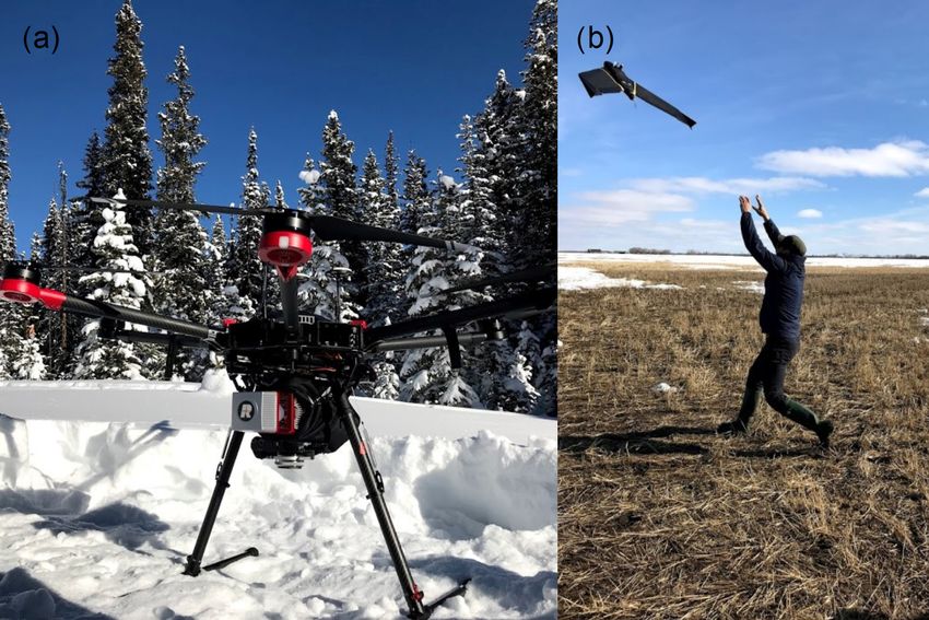
in this paper are (1) to evaluate the ability of UAV-lidar ver- Pro UAV platform (Fig. 2a). The miniVUX-1UAV utilises
sus UAV-SfM techniques for measuring snow depth in open a rotating mirror to provide a 360-degree line scan with a
and vegetated areas and (2) to articulate challenges and op- measurement rate of 100 KHz and up to five returns per shot
portunities for UAVs to map sub-canopy snow depth. with a 15 mm precision. The APX-20 provides positional ac-
curacy of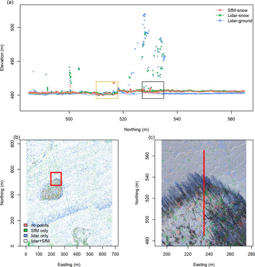
1922                          P. Harder et al.: Improving sub-canopy snow depth mapping with unmanned aerial vehicles

Figure 1. (a) Fortress Mountain Snow Observatory in Kananaskis, Alberta, Canada, and (b) Rosthern and (c) Clavet prairie study locations
in Saskatchewan, Canada. Data collection was centred on Fortress Ridge (ridgeline in background centre), an area of high topographic
variability and a mix of dense forests and clearings. The Rosthern photo highlights the low vertical relief of upland areas and isolated
woodlands amongst cultivated fields. The Clavet photo highlights the transition zone between the open upland agricultural terrain and the
lower-elevation vegetated wetland.

                                                                       Satellite System (GNSS) surveys and manual measurements
                                                                       of snow depths with a ruler. The intention of the surveys
                                                                       was to validate the spatially distributed snow depth retrievals,
                                                                       and transects were selected in a manner for the surveyor(s)
                                                                       to efficiently sample the greatest variety of vegetation types
                                                                       and gradients. A Leica GS16 base/rover kit provided a real-
                                                                       time kinematic (RTK) survey solution to survey points. The
                                                                       3D uncertainty of the relative position between the base and
                                                                       rover was computed in real time to be < ± 1.5 cm, which
                                                                       accounts for errors in signal strength, satellite coverage,
                                                                       and instrument precision. RTK signal quality can degrade
                                                                       in forests, but only points with carrier-phase RTK solutions
                                                                       were used in this analysis, so all survey points are of consis-
                                                                       tent quality irrespective of vegetation cover. Post-processing
Figure 2. UAV-lidar platform: RIEGL miniVUX-1UAV mounted               of the GNSS data used the Canadian Geodetic Survey of Nat-
on DJI M600 Pro (a). UAV-SfM platform: senseFly eBee X (b).            ural Resources Canada’s precise point positioning (PPP) on-
                                                                       line tool (Natural Resources Canada, 2020) to define an ab-
                                                                       solute base station location. Due to multi-site logistics, the
lightweight payload on a fixed-wing platform allowed for the           base station location varied between flights, collection pe-
efficient mapping of large areas. Overlap parameters were              riods ranged between 2.5 and 9 h, and PPP-computed stan-
generally 80 % for the longitudinal and 65 % for the lateral           dard deviations were consistently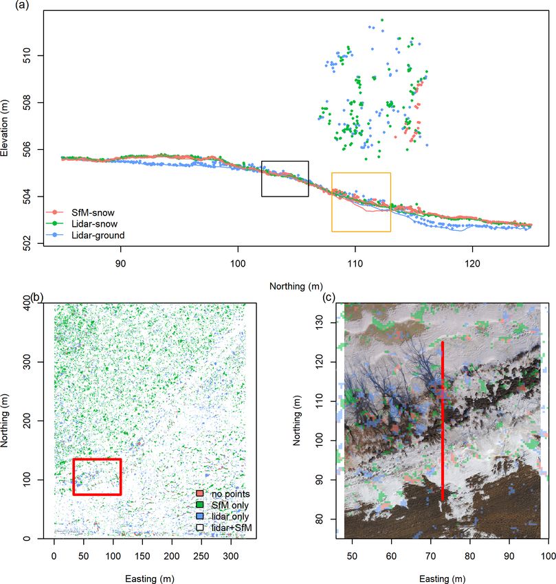
P. Harder et al.: Improving sub-canopy snow depth mapping with unmanned aerial vehicles                                       1923

Table 1. Summary of data collection campaign, September 2018 to   an absolute sensor position uncertainty of
1924                          P. Harder et al.: Improving sub-canopy snow depth mapping with unmanned aerial vehicles

Figure 3. Data processing workflows for lidar and SfM point cloud generation.

burg, 2019). A spatial resolution of 0.1 m was applied to all         3     Results
DEMs generated.

2.3.5   Error assessment                                              3.1    Accuracy of UAV-lidar versus UAV-SfM snow
                                                                             depth estimates
To assess the accuracy of UAV lidar and UAV SfM with re-
spect to observations, a DEM-based comparison was under-
taken. Snow and ground surface values were extracted from             An accuracy assessment comparing the snow depth from
the DEM raster cells for locations where a point was man-             UAV-lidar and UAV-SfM techniques to the manually sam-
ually surveyed and snow depth measured. The snow depth                pled ground surveys is shown in Fig. 5. UAV lidar has a con-
was calculated from the vertical difference between the snow          sistently lower error than UAV SfM in open environments
DEM and ground DEM. The influence of vegetation height                and mountain vegetation. The exception is prairie shrub veg-
on snow depth errors was also considered by segmenting                etation where the UAV-lidar RMSE is slightly larger than
the error metrics with respect to vegetation height (open             the UAV-SfM RMSE. The significance of the different rel-
2 m) derived from             ative RMSE values for prairie shrub vegetation is negligi-
the snow-free UAV-lidar scan. The classified vegetation maps          ble relative to the much larger differences noted in the other
and the location of all survey points are visualised in Fig. 4.       domains. UAV-lidar bias is consistently negative (−0.03 to
The error metrics employed to assess the differences between          −0.13 m), while the UAV-SfM bias is more variable and both
observations and estimates include the root mean square er-           positive and negative (0.08 to −0.14 m).
ror (RMSE) and the mean bias (mb) (Harder et al., 2016).                 The influence of vegetation on estimating snow depth from
                                                                      UAVs can be directly assessed by considering the errors asso-
2.3.6   Point cloud coverage                                          ciated with different vegetation classes (Fig. 5). When con-
                                                                      sidering UAV lidar, the errors are worse in the presence of
The continuity of bare-surface point density between UAV-             vegetation. Open prairie and open Fortress RMSE values are
lidar and UAV-SfM methods was quantified in order to inter-           similar (0.09 and 0.1 m RMSE, respectively), while vege-
pret how well the respective tools can sense sub-canopy sur-          tated sites have a larger error (0.13 to 0.17 m RMSE, re-
faces. All surveys with coincident UAV-lidar and UAV-SfM              spectively) with no observed dependency upon vegetation
flights were assessed with the LAStools (Isenburg, 2019)              class or type. The sample size of snow depth probe obser-
grid_metrics function to classify an area with >1 pt per              vations is smaller for vegetation sites than open sites, which
0.25 m−2 , and thereafter they were summarised as percent-            has implications for error metrics – outliers will have greater
age areas of each study site with >1 pt per 0.25 m−2 with             weight. The UAV lidar is equally successful at penetrating
respect to technique. This is a rough metric of DEM quality           the open, leaf-off deciduous tree canopy at the prairie sites
as it quantifies the relative amount of interpolation needed to       as the closed, needleleaf canopy at the Fortress site, based on
translate a point cloud to a continuous surface.                      the similar RMSE values within each site’s tree vegetation
                                                                      class. The UAV-lidar RMSE for shrub and tree vegetation
                                                                      classes at the Fortress and prairie sites are within 0.04 m. For
                                                                      UAV SfM the errors differ widely for various vegetation cov-
                                                                      ers. The open vegetation has a large RMSE range between

The Cryosphere, 14, 1919–1935, 2020                                                      https://doi.org/10.5194/tc-14-1919-2020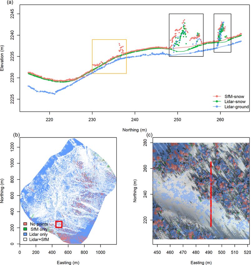
P. Harder et al.: Improving sub-canopy snow depth mapping with unmanned aerial vehicles                                                  1925

Figure 4. Fortress (a), Rosthern (b), and Clavet (c) study sites classified by vegetation height derived from snow-free (ground) UAV lidar into
open (0.5 and 2 m) domains. Red points identify locations of manual snow depth survey observations
sampled over the course of the data collection campaign. Black lines in the Fortress map are 50 m elevation contours.

                                                                             Snow depth is estimated from differencing the snow and
                                                                          ground DEMs. Therefore, the uncertainty of the snow depth
                                                                          is a propagation of the error of both the snow and ground
                                                                          DEMs. To distinguish which DEM may contribute more to
                                                                          the snow depth error, the remotely sensed surface elevations
                                                                          were compared to the surface elevations from manual GNSS
                                                                          surveys using boxplots (Fig. 6). The boxplots in Fig. 6 illus-
                                                                          trate that the UAV-SfM snow-surface elevations have errors
                                                                          consistently greater than the corresponding UAV-lidar sur-
                                                                          faces at Fortress. In the prairie snow-surface case, the me-
                                                                          dian RMSE is consistently lower for UAV SfM than UAV
                                                                          lidar, but the UAV SfM does have more variability in its er-
                                                                          rors. The ground surface was only available from UAV lidar
                                                                          for this study, so no corresponding UAV-SfM ground surface
                                                                          analysis is available. The snow-free UAV-lidar survey has a
                                                                          consistently higher or more variable RMSE than the snow
                                                                          surfaces (with the exception of the open prairie and open and
                                                                          tree Fortress UAV SfM).
Figure 5. Comparison of snow depth observations from snow
probes and snow depth estimates from UAV techniques. Plots are            3.2   Point cloud coverage
segmented within each vegetation class (rows), site (columns), and
observation method (colours).                                             The quality of a remotely sensed snow depth estimate is di-
                                                                          rectly tied to how much interpolation is required to fill gaps
                                                                          in a point cloud. The point clouds were classified into areas
                                                                          where >1 pt per 0.25 m−2 existed for each technique. Exam-
sites (0.1 m in prairie and 0.3 m in Fortress) while vegetation           ples of this approach are visualised for the Fortress, Rosth-
class RMSEs range from 0.13 to 0.33 m.                                    ern, and Clavet sites on 14 February and 18 and 20 March
   UAV SfM reports slightly better metrics than UAV lidar                 2019 survey dates in Figs. 7–9, respectively. At the Fortress
in the prairie shrub case: the difference between these tech-             site (Fig. 7b), the large areas of lidar-only points (blue) cor-
niques is only 0.04 m, which is within the ±0.025 m obser-                respond to areas of forest cover as the UAV-SfM technique
vational uncertainty of the GNSS survey equipment used in                 could not reliably return surface points with a density >1 pt
this project. The influence of vegetation type is apparent in             per 0.25 m−2 , while the UAV lidar could. At Fortress, UAV
the UAV-SfM tree class, where the dense needleleaf forest at              lidar had >1 pt per 0.25 m−2 for 93 % of the area of inter-
Fortress has a higher RMSE (0.33 m) than the leaf-off decid-              est versus 54 % for UAV SfM. Considering the black poly-
uous trees in the prairies (0.2 m). Overall, UAV lidar tends to           gons in the Fig. 7a transect, the lack of sub-canopy points
consistently have lower RMSEs than UAV SfM, which pro-                    identified within the tree vegetation class results in an inter-
vides confidence in this technique for sub-canopy snow depth              polated snow surface that is erroneously deep under trees,
mapping.                                                                  completely missing the detection of the reduced snow depths

https://doi.org/10.5194/tc-14-1919-2020                                                          The Cryosphere, 14, 1919–1935, 2020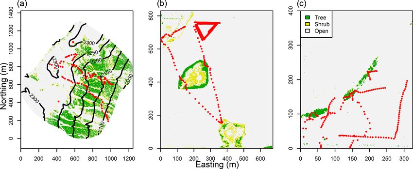
1926                            P. Harder et al.: Improving sub-canopy snow depth mapping with unmanned aerial vehicles

                                                                        greater uncertainty. There was ponded meltwater on the sur-
                                                                        face of the frozen ground and a frozen wetland water surface
                                                                        at the Clavet site on 20 March 2019, which is responsible for
                                                                        the many areas missing lidar points (green areas) in Fig. 9b.
                                                                        Water is a specular reflector; therefore, unless the lidar has a
                                                                        nadir perspective, water areas will appear as a gap in the point
                                                                        cloud. Fortunately, since water surfaces are flat, minimal in-
                                                                        terpolation artefacts remain when generating DEMs from the
                                                                        point clouds if the pond edges are sufficiently captured. The
                                                                        challenge in the Canadian Prairies, as seen in the black poly-
                                                                        gons in Figs. 8a and 9a, is in areas of thick but short vegeta-
                                                                        tion (shrub class) where both lidar pulses and SfM solutions
                                                                        interpret the vegetation surface as the top of the bare ground
                                                                        or snow surface, and therefore little difference exists between
                                                                        DEMs during all measurement periods. An additional chal-
                                                                        lenge of using the UAV-SfM technique is that large gaps in
                                                                        points appear beneath the tall wetland-edge vegetation, lead-
                                                                        ing to points, as visualised in orange polygons in the cross
Figure 6. Boxplots of RMSEs of UAV-estimated and RTK-surveyed           sections of Figs. 8a and 9a, where the estimated UAV-SfM
surface elevations segmented by surface condition, technique,           snow surface is below the UAV-lidar ground surface.
site, and vegetation classification. The error metrics approach the
±2.5 cm uncertainty of the RTK survey data (black line). Median
is indicated by the line within the box: the upper bound is the 75th
                                                                        4     Discussion
percentile, the lower bound is the 25th percentile, and whiskers rep-
resent the range of values beyond the box.
                                                                        4.1    UAV lidar is more accurate and consistent than
                                                                               UAV SfM

which are clearly detected (green line) around the base of              Snow depth mapping with UAVs has had widespread ap-
the trees by UAV lidar. The noisy UAV-SfM points in the                 plication in recent years (Bühler et al., 2016; Harder et al.,
middle of the slope (orange polygon) come from vegetation               2016; Vander Jagt et al., 2015; De Michele et al., 2016). The
adjacent to the transect. These vegetation points occupied a            emphasis has been on using SfM techniques to difference
larger space than the UAV lidar and intruded on the tran-               DEMs. One of the objectives of this work was to consider the
sect line. Therefore vegetation removal from this point in the          snow depth accuracies possible with the current state of the
transect led to a gap in the UAV-SfM point cloud but not the            art of UAV-SfM versus UAV-lidar platforms. What has been
UAV-lidar point cloud. Interpolating through the gap in the             demonstrated here is that while there are still errors in UAV
UAV-SfM point cloud at this point led to an underestimation             lidar (as with any measurement), they are smaller and more
of the snow surface. An additional challenge for UAV SfM is             consistent relative to UAV SfM. An unavoidable problem for
open areas with low surface contrast and surface homogene-              all SfM implementations, which is reflected in this work, is
ity, which resulted in large areas without point coverage on            that SfM can only sense the surface – whether that it is the
the northwest portion of the Fortress study area.                       ground/snow surface or the top of a vegetation canopy (West-
   The predominantly open nature of the prairie sites demon-            oby et al., 2012). This makes it fundamentally inappropriate
strates a minimal difference in point coverage between the              for sub-canopy mapping of snow. Sub-canopy snow depth
UAV-lidar and UAV-SfM techniques. The average extent of                 mapping with UAV SfM therefore becomes an exercise in in-
the study domain covered with a point density of >1 pt per              terpolating snow depth values observed in open areas without
0.25 m−2 for five coincident flights at prairie sites was com-          vegetation to areas with dense vegetation, rather than sens-
puted, resulting in the mean coverage of 92 % versus 83 %               ing the actual snow depth under the canopy. Open areas will
of the study area for UAV lidar and UAV SfM, respectively.              have greater snow depths than forest areas (Troendle, 1983;
As seen in Fig. 8 at the Rosthern site, the areas without               Swanson et al., 1986; Pomeroy et al., 2001; Mazzotti et al.,
UAV-lidar points include some wetland shrubs (green areas               2019), meaning UAV-SfM solutions, or any approach which
in Fig. 8b and c), but predominantly they are randomly dis-             requires interpolation of point cloud gaps beneath trees, will
tributed points. In contrast, UAV SfM is missing points from            overestimate snow (Zheng et al., 2016). The ability of UAV
areas where the snow surface is very uniform, in vegetated              lidar to map snow depths with and without canopy cover and
rings around wetlands, and in areas of dense vegetation (blue           capture tree wells with a RMSE ≤ 0.17 m is an improvement
areas in Fig. 8b and c). These gaps in the UAV-SfM point                on previous attempts. This RMSE is comparable to previous
clouds are interpolated and therefore will represent areas of           efforts with UAV SfM (Bühler et al., 2016; De Michele et al.,

The Cryosphere, 14, 1919–1935, 2020                                                        https://doi.org/10.5194/tc-14-1919-2020
P. Harder et al.: Improving sub-canopy snow depth mapping with unmanned aerial vehicles 1927
Figure 7. Fortress Ridge (14 February 2019) study site with an example (a) cross section with all points and the interpolated vegetation-free
surface (lines) for SfM-snow (red), lidar-snow (green), and lidar-ground (blue) surveys. The study area is classified by areas with greater
than 1 pt per 0.25 m−2 in (b) with respect to point clouds obtained from UAV-lidar and UAV-SfM techniques. In (a) black polygons highlight
areas of tree wells while the orange polygon highlights an area of UAV-SfM noise on a slope. The red inset polygon in (b) identifies the area
of the orthomosaics displayed in (c) with the same overlain transparent point type classification colour scheme as shown in (b). The red line
in (c) corresponds to the cross section plotted in (a).
2016; Harder et al., 2016), airborne SfM (Bühler et al., 2015; be similar between techniques, the ability of UAV lidar to
Nolan et al., 2015, Meyer and Skiles, 2019), and airborne sense a surface below vegetation is critical to develop a co-
lidar (Deems et al., 2013; Painter et al., 2016), which have herent snow-surface DEM. The point cloud cross section il-
been primarily focussed on mapping the snow depth of open lustrated in Fig. 7 emphasises these findings, highlighting
snow surfaces. Applications of airborne lidar to forested ar- the wider gaps in the UAV-SfM point cloud beneath indi-
eas report similar errors (Zheng et al., 2016; Currier et al., vidual trees that require interpolation over longer distances,
2019; Mazzotti et al., 2019), but the higher flight altitude which results in a greater potential for error. Features such as
of airborne platforms and their near-nadir perspective limit tree wells, where the snow depth decreases with proximity
point densities near tree centres that are necessary to capture to a tree due to interception/sublimation losses and radiative
tree wells. melting (Pomeroy and Gray, 1995; Musselman and Pomeroy,
2017), will be missed. An interesting dynamic of the RM-
4.2 Bare-surface point cloud coverage is critical SEs is that while lidar is comparable across all the sites and
vegetation categories, the UAV-SfM RMSE values are much
greater in the mountain domain. This is attributed to inter-
The increased continuous point coverage of UAV lidar is the
polation artefacts. In prairies where topography is fairly flat,
main advantage over UAV SfM when trying to map sub-
the interpolation of the few gaps can give a reasonable ap-
canopy snow depth. While snow depth accuracy at times can
https://doi.org/10.5194/tc-14-1919-2020 The Cryosphere, 14, 1919–1935, 20201928 P. Harder et al.: Improving sub-canopy snow depth mapping with unmanned aerial vehicles
Figure 8. Rosthern (18 March 2019) study site with an example (a) cross section with all points and the interpolated vegetation-free surface
(lines) for SfM-snow (red), lidar-snow (green), and lidar-ground (blue) surveys. The study area is classified by areas with greater than 1 pt
per 0.25 m−2 in (b) with respect to point clouds obtained from UAV-lidar and UAV-SfM techniques. In (a) the black polygon highlights areas
of dense shrubs while the orange polygon highlights interpolation artefacts of UAV SfM. The red inset polygon in (b) identifies the area of
the orthomosaics displayed in (c) with the same overlain transparent point type classification colour scheme as shown in (b). The red line in
(c) corresponds to the cross section plotted in (a).
proximation of the actual surfaces. In contrast, mountainous are presented here to exemplify analyses that are possible
regions have a much more complex topography, and the in- with UAV lidar.
terpolation of large gaps misses much of the small-scale to-
pography and snow–vegetation interaction features. Interpo- 4.3.1 Fortress snow depth change
lation works better between two points that are on the same
plane (prairies) rather than on a complex non-linear slope The differences between open and forest snow cover pro-
(mountains), and where gaps in the point cloud are smaller. cesses can be explored by examining the difference in snow
depth between the UAV-lidar scans that took place on 13
February and 25 April 2019 at Fortress. Over this interval,
4.3 Lidar snow depth maps and quantifying there was intermittent precipitation totaling approximately
snow–vegetation interactions 100 mm, measured at storage gauges within the study area.
The UAV-lidar measured change in snow depth visualises
The ability of UAV lidar to map sub-canopy snow depth is how snow–vegetation interactions translated this snowfall
established by the consistent error metrics reported, as well into a snow depth distribution change over a 2 month in-
as the continuous bare-surface point cloud coverage. The terval (Fig. 10). In the Fig. 10c cross section, there was ac-
dynamics of snow depth at snow and vegetation process- cumulation of up to 2 m over the September–April time pe-
resolving scales can therefore be examined. Two examples riod on lee slopes, while the upper windswept portions of
The Cryosphere, 14, 1919–1935, 2020 https://doi.org/10.5194/tc-14-1919-2020P. Harder et al.: Improving sub-canopy snow depth mapping with unmanned aerial vehicles 1929
Figure 9. Clavet (20 March 2019) study site with an example (a) cross section with all points and the interpolated vegetation-free surface
(lines) for SfM-snow (red), lidar-snow (green), and lidar-ground (blue) surveys. The study area is classified by areas with greater than 1 pt
per 0.25 m−2 in (b) with respect to point clouds obtained from UAV-lidar and UAV-SfM techniques. In (a) the black polygon highlights areas
of dense shrubs while the orange polygon highlights interpolation artefacts of the UAV SfM. The red inset polygon in (b) identifies the area
of the orthomosaics displayed in (c) with the same overlain transparent point type classification colour scheme as shown in (b). The red line
in (c) corresponds to the cross section plotted in (a).
the ridge demonstrate snow erosion between February and wind redistribution, and snow accumulation on the lee slope
April. The dynamics and extents of blowing snow sources greatly exceeds the observed precipitation.
(grey/red) and sinks (blue) are clearly visualised in Fig. 10a,
which closely match the findings of Schirmer and Pomeroy 4.3.2 Prairie peak snow depth and ablation patterns
(2020), who used SfM for the same study region. In the forest
the UAV lidar observed the increasing snow drifts on the tree In the prairies, wind redistribution is the main driver of snow
line (the krummholz and tree islands – blue areas on top of depth spatial variability. Areas of tall vegetation accumulate
facing slope in Fig. 10a). Within the forested (Fig. 10b) tran- wind-blown snow from open upwind sources and are typi-
sect, there is a general decline in snow depth from February cally associated with the deepest snowpacks. In the winter of
to April due to melt on a south facing slope (on the left of 2019, the chronology of snow, temperature, and wind events
the figure) and the development of tree wells in the middle of defined the final snow depth distribution (Fig. 11a). The UAV
the transect (orange polygons). The Fig. 10b transect demon- lidar flown on 13 March captures all of these interactions.
strates the lack of wind redistribution in the forest; snow ac- Deep snow drifts are found in the roadside ditches (linear fea-
cumulation is consistently observed to be less than precipita- tures of 1.5 m snow depth on the north and northwest corners
tion over the transect due to interception losses, while the Fig. 11a), on the edges of wetland vegetation (>1 m snow
Fig. 10c transect on the ridgeline demonstrates significant depths on edges of wetlands identified by red polygons in
Fig. 11a), and the development of a sastrugi dune complex
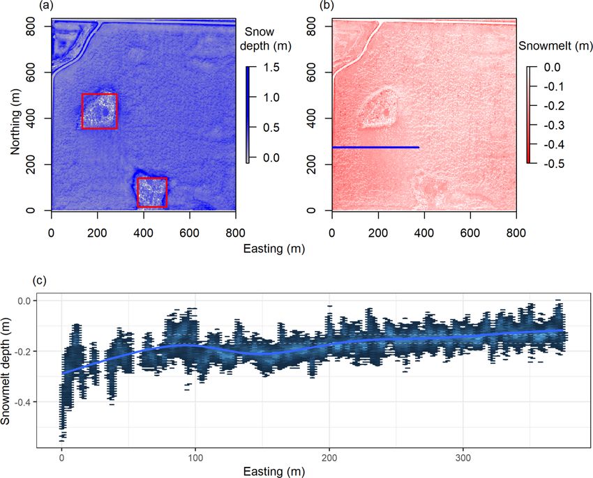
https://doi.org/10.5194/tc-14-1919-2020 The Cryosphere, 14, 1919–1935, 20201930 P. Harder et al.: Improving sub-canopy snow depth mapping with unmanned aerial vehicles
at the appropriate resolutions. First, the spatial variability of
albedo is a major driver of snowmelt. The greatest melt oc-
curs alongside the gravel-covered “grid” roads in the ditches
where road dust significantly lowers the albedo, thereby ac-
celerating the melt of the deep snowpacks. Moving eastward
from the road ditches into the open fields, there is a de-
crease in snowmelt depth in the overall scene, visualised in
the Fig. 11c transect. This pattern is likely due to the redistri-
bution of dust from the grid roads to the open-field snow sur-
face by the prevailing westerly winds. A snow-surface dust
concentration gradient develops over the winter with higher
concentrations of dust, and therefore lower albedo (Woo and
Dubreuil, 1985), in the west than the east. This increase in
albedo, and therefore decrease in solar radiation available to
melt snow, corresponds to a decrease in the snowmelt rate
(Fig. 11c), moving easterly away from the grid road. Sec-
ond, the spatial variability of snowpack cold content influ-
ences melt rates in the early part of the melt season. Within
the agricultural field, the sastrugi drifts are not melting due
Figure 10. (a) UAV-lidar-derived snow depth difference between to the larger cold content of the deep cold snowdrifts rela-
13 February and 25 April 2019. Green and yellow lines in (a) cor- tive to the smaller cold content of the shallower surrounding
respond to the forest and ridge line transect locations for cross sec- snowpacks. This is also prevalent in the non-melting deep
tions in (b) and (c), respectively. Cross-section figures plot the 0.5 m
snowdrifts at the vegetated wetland edges. With UAV lidar,
wide point cloud cross section from the 19 September 2018 snow-
free scan (black points) to show the point cloud and the processed
a complete picture of the early and asynchronous snowmelt
surfaces of the UAV-lidar scans of the bare ground from 19 Septem- processes is possible. If reliant on UAV SfM, the interpola-
ber 2018 (red) and the snow surface from 14 February 2019 (green) tion needed to fill gaps in the point cloud, near vegetation,
and 25 April 2019 (blue). Orange polygons in (b) highlight loca- and the tops of the sastrugi will obscure the full spatial pat-
tions of tree wells. tern of snow depth change that conveys the heterogeneity of
ablation processes. The high spatial resolution and vertical
accuracy of UAV lidar are required to capture these spatial
in open areas (parabolic dune shapes and small-scale snow patterns as the length scales of the snow-surface features of
depth variability in middle of Fig. 11a). Areas that the UAV interest are small; i.e. sastrugi drifts are on the metre scale,
lidar was able to measure correspond to areas where snow and their changes at daily timesteps are on the centimetre
depth is the deepest and has important snow–vegetation in- scale.
teractions. In contrast UAV SfM struggles with sensing snow The processes visualised in the Fortress and Rosthern ex-
depth on the edges of wetlands as seen by the concentration amples are not new, but the value of UAV lidar is that spatial
of lidar-only (blue) areas on the wetland edge in the Rosth- patterns and changes can be observed across complex land-
ern study area (wetland area highlighted by red polygon in scapes and vegetation gradients with a consistent resolution
Fig. 8b). In the prairies, mapping the areas with deep snow is and accuracy. UAV lidar will therefore be a powerful tool to
critical as the deepest snow areas are the ones that dominate understand landscape-scale snow–vegetation interactions, as
runoff generation and runoff contributing areas, are critical well as to make a core contribution to the validation and im-
for ephemeral wetland ecology, and have the longest snow provement of distributed snow process modelling.
cover duration with the related runoff timing implications
(Fang and Pomeroy, 2009; Pomeroy et al., 2014). 4.4 Are the costs and logistics of UAV lidar worth it?
Prairie snowpacks are shallow, leading Harder et al. (2016)
to conclude that UAV SfM was unable to capture snow abla- UAV lidar, relative to UAV SfM, provides the ability to mea-
tion patterns as the signal-to-noise ratio in the open domain sure snow depth below vegetation canopies, but it does come
was too large, and vegetated area errors were not consid- at a higher cost and logistical complexity. There are many
ered. With the demonstrated ability of UAV lidar to consis- similarities between the approaches, and one commonality is
tently map shallow snow in open areas and deep snow in the that both UAV lidar and UAV SfM require access to a GNSS
vegetated areas, this can be reattempted. Consider the dif- solution to geolocate point clouds in absolute space. The Le-
ference in snow depth between 18 and 23 March (Fig. 11b), ica GS16 package used here is on the expensive side of the
which represents the earliest part of the active melt period in spectrum (CAD 70 000), and cheaper equipment, subscrip-
this particular snowmelt season. Two examples of the spa- tion to virtual reference station networks if available in the
tial variability of process interactions can now be visualised study area (requires only a rover and not a base station), and
The Cryosphere, 14, 1919–1935, 2020 https://doi.org/10.5194/tc-14-1919-2020P. Harder et al.: Improving sub-canopy snow depth mapping with unmanned aerial vehicles 1931 Figure 11. Peak snow depth at the Rosthern site from the UAV-lidar scan on 13 March 2019 (a) and snow melt depth difference from the UAV-lidar scans on 18 and 22 March 2019 (b). Snow depth change (c) over a transect (blue line in b) are plotted with a hex plot (to show variability) and smoothed line (to show mean change). Red polygons in (a) highlight wetland areas. equipment rentals are all viable alternatives to lower costs. UAV lidar and UAV SfM are more subtle than the stark cost The main cost difference between UAV-lidar and UAV-SfM difference. UAV SfM simply requires a UAV platform and platforms is therefore in terms of the UAV sensor payload. A camera in its basic configuration, and therefore small, high- plethora of UAV-SfM options with and without RTK or PPK endurance platforms with small batteries can be easily de- photo geotagging are available and can range from small in- ployed to map large areas. In contrast, most current UAV- expensive systems like consumer grade UAVs (DJI Phantom lidar configurations need larger platforms that require more 3 < CAD 2000) to more expensive options like the senseFly cycles of large battery sets to cover similar areas, which eBee X PPK system (CAD 30 000) used here. Current in- represents a logistical challenge in keeping batteries warm tegrated lidar systems suited to UAV snow mapping (laser and charged in cold and remote areas. Previous UAV-SfM wavelengths
1932                         P. Harder et al.: Improving sub-canopy snow depth mapping with unmanned aerial vehicles

4.5    Ongoing challenges and future research needs                errors. Unfortunately, this may not be feasible if the critical
                                                                   wetland areas are inundated as is often the case in the Cana-
The ability of UAV lidar to resolve sub-canopy snow depths         dian Prairies in spring.
is not without challenges. Precise classification of surface          Mapping sub-canopy snow depth is important, but the ul-
points from snow and ground scans are needed to resolve the        timate variable of interest is SWE. The challenge is that at
snow depth at the resolutions needed to confidently capture        snow–vegetation interaction scales there may be significant
snow–vegetation interactions. Where there are dense shrubs,        variability from snow pack densification being driven by dif-
the last returns will not necessarily be the snow or ground        ferent processes across a landscape (Faria et al., 2000). Den-
surface, and therefore last-return methods common to air-          sification from wind packing is prevalent in open areas ver-
borne applications will not be appropriate. Sub-canopy snow        sus metamorphic densification due to temperature gradients
depth mapping requires careful selection of the appropriate        in sheltered sub-canopy areas (López-Moreno et al., 2013).
point cloud classification and filtering tools and associated      Current methods of modelling or measuring snow density
parameters to be able to reliably detect the sub-canopy bare       are not without problems at these small scales. Modelling
surface and achieve the desired quality and precision in a fi-     snow density will impose conceptual understandings of these
nal point cloud. To preserve the small-scale surface variabil-     processes (Raleigh and Small, 2017; Wetlaufer et al., 2016),
ity, point cloud processing will be less efficient as all points   which may be inappropriate for the small-scale features that
need consideration, and the focus on small-scale features will     need to be represented – these may miss mechanical densi-
at times lead to erroneous inclusion of points representing        fication from snow clumps unloading or dripping from the
large-scale non-surface objects. The algorithm and param-          canopy for example. Observational approaches are also a
eter decisions also have to be adjusted for each flight and        challenge as typical in situ measurements are destructive,
site/environment for UAV SfM due to the variable quality           limited in extent, and often too limited to develop robust rela-
and noise of the generated point cloud.                            tionships of depth versus density at both the small local and
   An especially challenging feature in resolving a ground         large landscape scales needed (Kinar and Pomeroy, 2015a;
surface is the presence of low and dense vegetation such as        Pomeroy and Gray, 1995). Opportunities may be available to
shrubs and wetland reeds. This is evident in looking in the        pair UAV lidar with other UAV-borne sensors such as passive
centre of the wetland zones (red polygons) of Fig. 11a where       gamma ray or snow acoustics (Kinar and Pomeroy, 2015b)
there are negative snow depths calculated. In this case, the li-   to non-destructively develop high spatial and temporal res-
dar pulses cannot penetrate the dense vegetation to the under-     olution estimates of snow density and ultimately the water
lying ground surface, and the classified bare-ground points        equivalent.
have a positive bias. As snow accumulates, the reeds com-
press and shrubs bend over to the extent that the correspond-
ing snow surface is below the biased bare-ground surface.          5   Conclusions
In the examples presented above, the areas of negative snow
are limited to areas where snow depth is relatively shallow        Remote sensing techniques to determine snow–vegetation
in comparison to the deep snow on the wetland edges. This          interactions have consistently been challenged by the pres-
challenge might also be apparent in other regions such as the      ence of vegetation. This work directly considers emerging
Arctic tundra, where shrub bending and burial by snow have         UAV-lidar and UAV-SfM techniques to address this gap in
been extensively documented (Pomeroy et al., 2006; Sturm           observational capacity. Based upon extensive data collec-
et al., 2005). While shrubs are much sparser than wetland          tion at a variety of sites and snow conditions with varying
reeds, their dynamic change in height and potential to posi-       snow–vegetation processes, the ability of UAV lidar to mea-
tively bias the ground surface extraction will increase uncer-     sure sub-canopy snow depth is demonstrated. UAV lidar pro-
tainty of snow depth estimation in these hydrologically sig-       vides snow depth estimates with RMSEs
P. Harder et al.: Improving sub-canopy snow depth mapping with unmanned aerial vehicles 1933 catchment extents (i.e.
1934                            P. Harder et al.: Improving sub-canopy snow depth mapping with unmanned aerial vehicles

Egli, L., Jonas, T., Grünewald, T., Schirmer, M., and Burlando, P.:        https://rapidlasso.com/2018/12/27/scripting-lastools-to-create-
   Dynamics of snow ablation in a small Alpine catchment observed          a-clean-dtm-from-noisy-photogrammetric-point-cloud/           (last
   by repeated terrestrial laser scans, Hydrol. Process., 26, 1574–        access: 29 May 2019), 2018.
   1585, https://doi.org/10.1002/hyp.8244, 2012.                        Isenburg, M.: LAStools – efficient tools for LiDAR processing,
Essery, R., Li, L., and Pomeroy, J. W.: A distributed model of blow-       version 190812, available at: http://lastools.org (last access:
   ing snow over complex terrain, Hydrol. Process., 13, 2423–2438,         10 June 2020), 2019.
   1999.                                                                Jonas, T., Marty, C., and Magnusson, J.: Estimating the
Fang, X. and Pomeroy, J. W.: Modelling blowing snow redistribu-            snow water equivalent from snow depth measure-
   tion to prairie wetlands, Hydrol. Process., 23, 2557–2569, 2009.        ments in the Swiss Alps, J. Hydrol., 378, 161–167,
Faria, D., Pomeroy, J. W., and Essery, R. L. H.: Effect of covari-         https://doi.org/10.1016/j.jhydrol.2009.09.021, 2009.
   ance between ablation and snow water equivalent on depletion of      Kinar, N. J. and Pomeroy, J. W.: Automated Determination of Snow
   snow-covered area in a forest, Hydrol. Process., 14, 2683–2695,         Water Equivalent by Acoustic Reflectometry, IEEE T. Geosci.
   2000.                                                                   Remote Sens., 47, 3161–3167, 2009.
Gelfan, A., Pomeroy, J. W., and Kuchment, L. S.: Modeling Forest        Kinar, N. J. and Pomeroy, J. W.: Measurement of the physi-
   Cover Influences on Snow Accumulation, Sublimation, and Melt,           cal properties of the snowpack, Rev. Geophys., 53, 481–544,
   J. Hydrometeorol., 5, 785–803, 2004.                                    https://doi.org/10.1002/2015RG000481, 2015a.
Goodison, B. E., Glynn, J. E., Harvey, K. D., and Slater, J. E.: Snow   Kinar, N. J. and Pomeroy, J. W.: SAS2: the system for
   Surveying in Canada: A Perspective, Can. Water Resour. J., 12,          acoustic sensing of snow, Hydrol. Process., 29, 4032–4050,
   27–42, https://doi.org/10.4296/cwrj1202027, 1987.                       https://doi.org/10.1002/hyp.10535, 2015b.
Grünewald, T., Schirmer, M., Mott, R., and Lehning, M.: Spa-            King, J., Pomeroy, J. W., Gray, D. M., Fierz, C., Fohn, P. M. B.,
   tial and temporal variability of snow depth and ablation rates          Harding, R. J., Jordan, R., Martin, E., and Pluss, C.: Snow – at-
   in a small mountain catchment, The Cryosphere, 4, 215–225,              mosphere energy and mass balance, in: Snow and Climate: Phys-
   https://doi.org/10.5194/tc-4-215-2010, 2010.                            ical Processes, Surface Energy Exchange and Modeling, edited
Harder,     P.:    UAV      Snow      Depth     Analysis,     Zenodo,      by: Armstrong, R. and Brun, E., Cambridge University Press,
   https://doi.org/10.5281/zenodo.3804691, 2020.                           70–124, 2008.
Harder, P., Schirmer, M., Pomeroy, J., and Helgason, W.: Accuracy       Liston, G. E. and Hiemstra, C. A.: Representing Grass- and Shrub-
   of snow depth estimation in mountain and prairie environments           Snow-Atmosphere Interactions in Climate System Models, J.
   by an unmanned aerial vehicle, The Cryosphere, 10, 2559–2571,           Clim., 24, 2061–2079, https://doi.org/10.1175/2010JCLI4028.1,
   https://doi.org/10.5194/tc-10-2559-2016, 2016.                          2011.
Harder, P., Helgason, W. D., and Pomeroy, J. W.: Model-                 López-Moreno, J. I., Fassnacht, S. R., Heath, J. T., Mussel-
   ing the Snowpack Energy Balance during Melt under Ex-                   man, K. N., Revuelto, J., Latron, J., Morán-tejeda, E., and
   posed Crop Stubble, J. Hydrometeorol., 19, 1191–1214,                   Jonas, T.: Small scale spatial variability of snow density and
   https://doi.org/10.1175/jhm-d-18-0039.1, 2018.                          depth over complex alpine terrain: Implications for estimat-
Harder, P., Pomeroy, J., and Helgason, W.: Unmanned aerial ve-             ing snow water equivalent, Adv. Water Resour., 55, 40–52,
   hicle structure from motion and lidar data for sub-canopy               https://doi.org/10.1016/j.advwatres.2012.08.010, 2013.
   snow depth mapping, Federated Research Data Repository,              Mazzotti, G., Currier, W. R., Deems, J. S., Pflug, J. M., Lundquist, J.
   https://doi.org/10.20383/101.0193, 2020.                                D., and Jonas, T.: Revisiting Snow Cover Variability and Canopy
Harpold, A., Guo, Q., Molotoch, Q., Brooks, P. D., Bales, R.,              Structure Within Forest Stands: Insights From Airborne Lidar
   Fernandez-Diaz, J. C., Musselman, K. N., Swetnam, T. L., Kirch-         Data, Water Resour. Res., 55, 6198–6216, 2019.
   ner, P. B., Meadows, M. W., Flanagan, J., and Lucas, R.: LiDAR-      Meyer, J. and Skiles, S. M.: Assessing the ability of Struc-
   derived snowpack data sets for mixed conifer forests across             ture from Motion to map high resolution snow surface
   the Western United States, Water Resour. Res., 50, 2749–2755,           elevations in complex terrain: A case study from Sena-
   https://doi.org/10.1002/2013WR013935, 2014.                             tor Beck Basin, CO, Water Resour. Res., 55, 6596–6605,
Hedrick, A. R., Marks, D., Havens, S., Robertson, M., Johnson,             https://doi.org/10.1029/2018WR024518, 2019.
   M., Sandusky, M., Marshall, H.-P., Kormos, P. R., Bormann, K.        Molotch, N. P. and Bales, R. C.: SNOTEL representativeness in
   J., and Painter, T. H.: Direct insertion of NASA Airborne Snow          the Rio Grande headwaters on the basis of physiographics and
   Observatory-derived snow depth time series into the iSnobal en-         remotely sensed snow cover persistence, Hydrol. Process., 20,
   ergy balance snow model, Water Resour. Res., 54, 8045–8063,             723–739, https://doi.org/10.1002/hyp.6128, 2006.
   https://doi.org/10.1029/2018WR023190, 2018.                          Mott, R., Egli, L., Grünewald, T., Dawes, N., Manes, C., Bavay, M.,
Hedstrom, N. R. and Pomeroy, J. W.: Measurements and modelling             and Lehning, M.: Micrometeorological processes driving snow
   of snow interception in the boreal forest, Hydrol. Process., 12,        ablation in an Alpine catchment, The Cryosphere, 5, 1083–1098,
   1611–1625, 1998.                                                        https://doi.org/10.5194/tc-5-1083-2011, 2011.
Helms, D., Phillips, S. E., and Reich, P. F.: The History of Snow       Musselman, K. N. and Pomeroy, J. W.: Estimation of Needle-
   Survey and Water Supply Forecasting Interviews with U.S. De-            leaf Canopy and Trunk Temperatures and Longwave Con-
   partment of Agriculture Pioneers., United States Department of          tribution to Melting Snow, J. Hydrometeorol., 18, 555–572,
   Agriculture, Natural Resoruces Conservation Service, 321 pp.,           https://doi.org/10.1175/JHM-D-16-0111.1, 2017.
   2008.                                                                Musselman, K. N., Molotch, N. P., and Brooks, P.: Effects
Isenburg, M.: Scripting LAStools to Create a Clean DTM                     of vegetation on snow accumulation and ablation in a mid-
   from Noisy Photogrammetric Point Cloud, available at:

The Cryosphere, 14, 1919–1935, 2020                                                           https://doi.org/10.5194/tc-14-1919-2020
P. Harder et al.: Improving sub-canopy snow depth mapping with unmanned aerial vehicles                                               1935

  latitude sub-alpine forest, Hydrol. Process., 22, 2767–2776,         Smith, C. D., Kontu, A., Laffin, R., and Pomeroy, J. W.: An as-
  https://doi.org/10.1002/hyp.7050, 2008.                                 sessment of two automated snow water equivalent instruments
Natural Resources Canada: Precise Point Positioning Online Tool,          during the WMO Solid Precipitation Intercomparison Experi-
  available at: https://webapp.geod.nrcan.gc.ca/geod/tools-outils/        ment, The Cryosphere, 11, 101–116, https://doi.org/10.5194/tc-
  ppp.php?locale=en, last access: 8 April 2020.                           11-101-2017, 2017.
Nolan, M., Larsen, C., and Sturm, M.: Mapping snow depth from          Shook, K. and Gray, D. M.: Small-Scale Spatial Structure of Shal-
  manned aircraft on landscape scales at centimeter resolution us-        low Snowcovers, Hydrol. Process., 10, 1283–1292, 1996.
  ing structure-from-motion photogrammetry, The Cryosphere, 9,         SPH Engineering: Universal Ground Control Station (UgCS) Soft-
  1445–1463, https://doi.org/10.5194/tc-9-1445-2015, 2015.                ware, Verison 3.4, Latvia, 2020.
Nolin, A. W.: Recent advances in remote sensing of seasonal snow,      Steppuhn, H. and Dyck, G. E.: Estimating True Basin Snowcover, in
  J. Glaciol., 56, 1141–1150, 2010.                                       Proceedings of Interdisciplinary Symposium on Advanced Con-
Painter, T. H., Berisford, D. F., Boardman, J. W., Bormann, K. J.,        cepts and Techniques in the Study of Snow and Ice Resourses,
  Deems, J. S., Gehrke, F., Hedrick, A., Joyce, M., Laidlaw, R.,          pp. 314–328, 1974.
  Marks, D., Mattmann, C., McGurk, B., Ramirez, P., Richard-           Sturm, M.: White water: Fifty years of snow research in WRR and
  son, M., Skiles, S. M. K., Seidel, F. C., and Winstral, A.: The         the outlook for the future, Water Resour. Res., 51, 4948–4965,
  Airborne Snow Observatory: Fusion of scanning lidar, imaging            https://doi.org/10.1002/2015WR017242, 2015.
  spectrometer, and physically-based modeling for mapping snow         Sturm, M., Douglas, T., Racine, C., and Liston, G.: Chang-
  water equivalent and snow albedo, Remote Sens. Environ., 184,           ing snow and shrub conditions affect albedo with
  139–152, https://doi.org/10.1016/j.rse.2016.06.018, 2016.               global implications, J. Geophys. Res., 110, G01004,
Parviainen, J. and Pomeroy, J. W.: Multiple-scale modelling of            https://doi.org/10.1029/2005JG000013, 2005.
  forest snow sublimation: initial findings, Hydrol. Process., 14,     Swanson, R. H., Golding, D. L., Rothwell, R. L., and Bernier, P.:
  2669–2681, 2000.                                                        Hydrologic effects of clear-cutting at Marmot Creek and Streeter
Pomeroy, J., Bewley, D., Essery, R., Hedstrom, N., Link, T.,              watersheds, Alberta, North. For. Centre, Can. For. Serv. Inf. Rep.
  Granger, R., Sicart J.-E., Ellis, C., and Janowicz, R.: Shrub tun-      NOR-X-278, 33, 1986.
  dra snowmelt, Hydrol. Process., 20, 923–941, 2006.                   Tinkham, W. T., Smith, A. M. S., Marshall, H. P., Link,
Pomeroy, J. W. and Gray, D. M.: Snow accumulation, relocation             T. E., Falkowski, M. J., and Winstral, A. H.: Quantifying
  and management, Science Report No. 7, National Hydrology Re-            spatial distribution of snow depth errors from LiDAR us-
  search Institute, Environment Canada, Saskatoon, SK, 1995.              ing Random Forest, Remote Sens. Environ., 141, 105–115,
Pomeroy, J. W., Gray, D. M., and Landine, P. G.: The Prairie Blow-        https://doi.org/10.1016/j.rse.2013.10.021, 2014.
  ing Snow Model: characteristics, validation, operation, J. Hy-       Troendle, C. A.: The potential for water yield augmentation from
  drol., 144, 165–192, 1993.                                              forest managament in the Rocky Mountain region, Water Resour.
Pomeroy, J. W., Holler, P., Marsh, P., Walker, D. A., and Williams,       Bull., 19, 359–373, 1983.
  M.: Snow vegetation interactions: issues for a new initiative, in    Trujillo, E., Ramirez, J. A., and Elder, K.: Topographic, meteoro-
  Soil, Vegetation, Atmosphere Transfer Schemes and Large Scale           logic, and canopy controls on the scaling characteristics of the
  Hydrological Models, 299–306, IAHS Publ. No. 270, 2001.                 spatial distribution of snow depth fields, Water Resour. Res., 43,
Pomeroy, J. W., Gray, D. M., Hedstrom, N. R., and Janowicz J. R.:         W07409, https://doi.org/10.1029/2006WR005317, 2007.
  Prediction of seasonal snow accumulation in cold climate forests,    Vander Jagt, B., Lucieer, A., Wallace, L., Turner, M., and
  Hydrol. Process., 16, 3543–3558, 2002.                                  Durand, D.: Snow Depth Retrieval with UAS Using
Pomeroy, J. W., Shook, K., Fang, X., Dumanski, S., Westbrook,             Photogrammetric Techniques, Geosciences, 5, 264–285,
  C., and Brown, T.: Improving and Testing the Prairie Hydrolog-          https://doi.org/10.3390/geosciences5030264, 2015.
  ical Model at Smith Creek Research Basin, Centre for Hydrol-         Westoby, M., Brasington, J., Glasser, N., Hambrey, M., and
  ogy Report: Report No. 14, Centre for Hydrology, University of          Reynolds, J.: “Structure-from-Motion” photogrammetry: A low-
  Saskatchewan, 2014.                                                     cost, effective tool for geoscience applications, Geomorphology,
Raleigh, M. S. and Small, E. E.: Snowpack density modeling                179, 300–314, https://doi.org/10.1016/j.geomorph.2012.08.021,
  is the primary source of uncertainty when mapping basin-                2012.
  wide SWE with lidar, Geophys. Res. Lett., 44, 3700–3709,             Wetlaufer, K., Hendrikx, J., and Marshall, L.: Spatial heterogene-
  https://doi.org/10.1002/2016GL071999, 2017.                             ity of snow density and its influence on snow water equiva-
Reba, M., Pomeroy, J. W., Marks, D., and Link, T. E.:                     lence estimates in a large mountainous basin, Hydrology, 3, 3,
  Estimating surface sublimation losses from snowpacks in                 https://doi.org/10.3390/hydrology3010003, 2016.
  a mountain catchment using eddy covariance and turbu-                Woo, M. and Dubreuil, M. A.: Empirical relationship between dust
  lent transfer calculations, Hydrol. Process., 26, 3699–3711,            content and Arctic snow albedo, Cold Reg. Sci. Technol., 10,
  https://doi.org/10.1002/hyp.8372, 2012.                                 125–132, https://doi.org/10.1016/0165-232X(85)90024-2, 1985.
Schirmer, M. and Pomeroy, J. W.: Processes governing snow              Zheng, Z., Kirchner, P. B., and Bales, R. C.: Topographic and
  ablation in alpine terrain – detailed measurements from the             vegetation effects on snow accumulation in the southern Sierra
  Canadian Rockies, Hydrol. Earth Syst. Sci., 24, 143–157,                Nevada: a statistical summary from lidar data, The Cryosphere,
  https://doi.org/10.5194/hess-24-143-2020, 2020.                         10, 257–269, https://doi.org/10.5194/tc-10-257-2016, 2016.
Schmidt, R. A.: Properties of Blowing Snow, Rev. Geophys. Sp.
  Phys., 20, 39–44, 1982.

https://doi.org/10.5194/tc-14-1919-2020                                                       The Cryosphere, 14, 1919–1935, 2020
You can also read