DeepSDF: Learning Continuous Signed Distance Functions for Shape Representation
←
→
Page content transcription
If your browser does not render page correctly, please read the page content below
DeepSDF: Learning Continuous Signed Distance Functions
                                                                           for Shape Representation
                                                 Jeong Joon Park1,3†         Peter Florence 2,3†        Julian Straub3    Richard Newcombe3          Steven Lovegrove3
                                                       1                                   2                                             3
                                                           University of Washington            Massachusetts Institute of Technology         Facebook Reality Labs
arXiv:1901.05103v1 [cs.CV] 16 Jan 2019

                                         Figure 1: DeepSDF represents signed distance functions (SDFs) of shapes via latent code-conditioned feed-forward decoder networks.
                                         Above images are raycast renderings of DeepSDF interpolating between two shapes in the learned shape latent space. Best viewed digitally.

                                                                    Abstract                                       1. Introduction
                                             Computer graphics, 3D computer vision and robotics                        Deep convolutional networks which are a mainstay of
                                         communities have produced multiple approaches to rep-                     image-based approaches grow quickly in space and time
                                         resenting 3D geometry for rendering and reconstruction.                   complexity when directly generalized to the 3rd spatial di-
                                         These provide trade-offs across fidelity, efficiency and com-             mension, and more classical and compact surface repre-
                                         pression capabilities. In this work, we introduce DeepSDF,                sentations such as triangle or quad meshes pose problems
                                         a learned continuous Signed Distance Function (SDF) rep-                  in training since we may need to deal with an unknown
                                         resentation of a class of shapes that enables high qual-                  number of vertices and arbitrary topology. These chal-
                                         ity shape representation, interpolation and completion from               lenges have limited the quality, flexibility and fidelity of
                                         partial and noisy 3D input data. DeepSDF, like its clas-                  deep learning approaches when attempting to either input
                                         sical counterpart, represents a shape’s surface by a con-                 3D data for processing or produce 3D inferences for object
                                         tinuous volumetric field: the magnitude of a point in the                 segmentation and reconstruction.
                                         field represents the distance to the surface boundary and the
                                                                                                                       In this work, we present a novel representation and ap-
                                         sign indicates whether the region is inside (-) or outside (+)
                                                                                                                   proach for generative 3D modeling that is efficient, expres-
                                         of the shape, hence our representation implicitly encodes a
                                                                                                                   sive, and fully continuous. Our approach uses the concept
                                         shape’s boundary as the zero-level-set of the learned func-
                                                                                                                   of a SDF, but unlike common surface reconstruction tech-
                                         tion while explicitly representing the classification of space
                                                                                                                   niques which discretize this SDF into a regular grid for eval-
                                         as being part of the shapes interior or not. While classical
                                                                                                                   uation and measurement denoising, we instead learn a gen-
                                         SDF’s both in analytical or discretized voxel form typically
                                                                                                                   erative model to produce such a continuous field.
                                         represent the surface of a single shape, DeepSDF can repre-
                                         sent an entire class of shapes. Furthermore, we show state-                   The proposed continuous representation may be intu-
                                         of-the-art performance for learned 3D shape representation                itively understood as a learned shape-conditioned classifier
                                         and completion while reducing the model size by an order                  for which the decision boundary is the surface of the shape
                                         of magnitude compared with previous work.                                 itself, as shown in Fig. 2. Our approach shares the genera-
                                                                                                                   tive aspect of other works seeking to map a latent space to
                                                                                                                   a distribution of complex shapes in 3D [54], but critically
                                             † Work performed during internship at Facebook Reality Labs.          differs in the central representation. While the notion of an

                                                                                                               1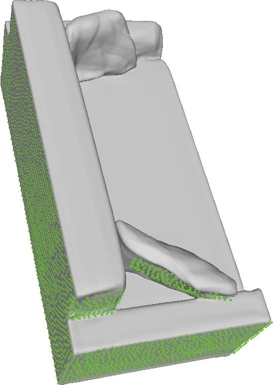
Decision
limitations in expressing continuous surfaces with complex
boundary topologies.
of implicit
surface
Point-based. A point cloud is a lightweight 3D representa-
tion that closely matches the raw data that many sensors (i.e.
LiDARs, depth cameras) provide, and hence is a natural fit
(a) for applying 3D learning. PointNet [38, 39], for example,
uses max-pool operations to extract global shape features,
and the technique is widely used as an encoder for point
generation networks [57, 1]. There is a sizable list of re-
lated works to the PointNet style approach of learning on
point clouds. A primary limitation, however, of learning
with point clouds is that they do not describe topology and
(b) (c) are not suitable for producing watertight surfaces.
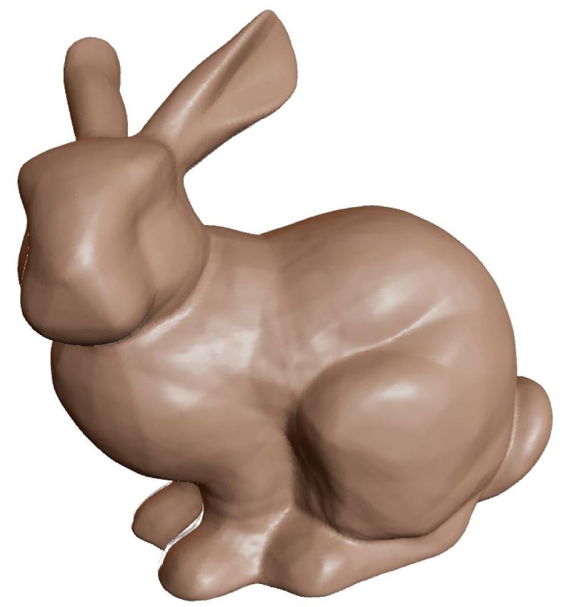
Figure 2: Our DeepSDF representation applied to the Stanford
Mesh-based. Various approaches represent classes of sim-
Bunny: (a) depiction of the underlying implicit surface SDF = 0 ilarly shaped objects, such as morphable human body parts,
trained on sampled points inside SDF < 0 and outside SDF > 0 with predefined template meshes and some of these models
the surface, (b) 2D cross-section of the signed distance field, (c) demonstrate high fidelity shape generation results [2, 34].
rendered 3D surface recovered from SDF = 0. Note that (b) and Other recent works [3] use poly-cube mapping [51] for
(c) are recovered via DeepSDF. shape optimization. While the use of template meshes is
convenient and naturally provides 3D correspondences, it
can only model shapes with fixed mesh topology.
implicit surface defined as a SDF is widely known in the Other mesh-based methods use existing [48, 36] or
computer vision and graphics communities, to our knowl- learned [22, 23] parameterization techniques to describe 3D
edge no prior works have attempted to directly learn contin- surfaces by morphing 2D planes. The quality of such repre-
uous, generalizable 3D generative models of SDFs. sentations depends on parameterization algorithms that are
Our contributions include: (i) the formulation of gen- often sensitive to input mesh quality and cutting strategies.
erative shape-conditioned 3D modeling with a continuous To address this, recent data-driven approaches [57, 22] learn
implicit surface, (ii) a learning method for 3D shapes based the parameterization task with deep networks. They report,
on a probabilistic auto-decoder, and (iii) the demonstration however, that (a) multiple planes are required to describe
and application of this formulation to shape modeling and complex topologies but (b) the generated surface patches
completion. Our models produce high quality continuous are not stitched, i.e. the produced shape is not closed. To
surfaces with complex topologies, and obtain state-of-the- generate a closed mesh, sphere parameterization may be
art results in quantitative comparisons for shape reconstruc- used [22, 23], but the resulting shape is limited to the topo-
tion and completion. As an example of the effectiveness logical sphere. Other works related to learning on meshes
of our method, our models use only 7.4 MB (megabytes) propose to use new convolution and pooling operations for
of memory to represent entire classes of shapes (for exam- meshes [17, 53] or general graphs [9].
ple, thousands of 3D chair models) – this is, for example, Voxel-based. Voxels, which non-parametrically describe
less than half the memory footprint (16.8 MB) of a single volumes with 3D grids of values, are perhaps the most natu-
uncompressed 5123 3D bitmap. ral extension into the 3D domain of the well-known learning
paradigms (i.e., convolution) that have excelled in the 2D
2. Related Work image domain. The most straightforward variant of voxel-
based learning is to use a dense occupancy grid (occupied /
We review three main areas of related work: 3D rep-
not occupied). Due to the cubically growing compute and
resentations for shape learning (Sec. 2.1), techniques for
memory requirements, however, current methods are only
learning generative models (Sec. 2.2), and shape comple-
able to handle low resolutions (1283 or below). As such,
tion (Sec. 2.3).
voxel-based approaches do not preserve fine shape details
[56, 14], and additionally voxels visually appear signifi-
2.1. Representations for 3D Shape Learning
cantly different than high-fidelity shapes, since when ren-
Representations for data-driven 3D learning approaches dered their normals are not smooth. Octree-based methods
can be largely classified into three categories: point-based, [52, 43, 26] alleviate the compute and memory limitations
mesh-based, and voxel-based methods. While some appli- of dense voxel methods, extending for example the ability to
cations such as 3D-point-cloud-based object classification learn at up to 5123 resolution [52], but even this resolution
are well suited to these representations, we address their is far from producing shapes that are visually compelling.
2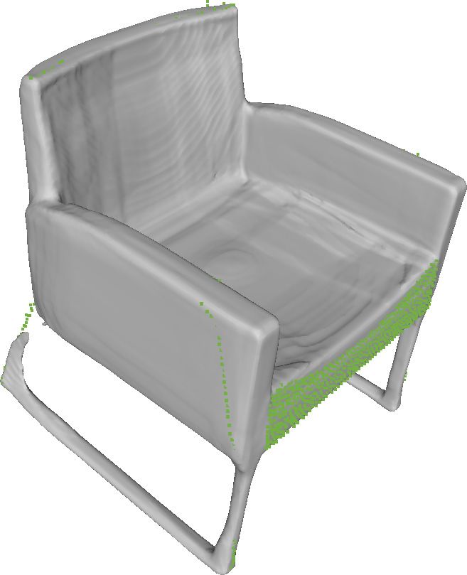
Aside from occupancy grids, and more closely related to           sively studied in [42, 8, 40], for applications including noise
our approach, it is also possible to use a 3D grid of vox-           reduction, missing measurement completions, and fault de-
els to represent a signed distance function. This inherits           tections. Recent approaches [7, 20] extend the technique by
from the success of fusion approaches that utilize a trun-           applying deep architectures. Throughout the paper we re-
cated SDF (TSDF), pioneered in [15, 37], to combine noisy            fer to this class of networks as auto-decoders, for they are
depth maps into a single 3D model. Voxel-based SDF repre-            trained with self-reconstruction loss on decoder-only archi-
sentations have been extensively used for 3D shape learning          tectures.
[59, 16, 49], but their use of discrete voxels is expensive in
memory. As a result, the learned discrete SDF approaches             2.3. Shape Completion
generally present low resolution shapes. [30] reports vari-             3D shape completion related works aim to infer unseen
ous wavelet transform-based approaches for distance field            parts of the original shape given sparse or partial input ob-
compression, while [10] applies dimensionality reduction             servations. This task is anaologous to image-inpainting in
techniques on discrete TSDF volumes. These methods en-               2D computer vision.
code the SDF volume of each individual scene rather than a              Classical surface reconstruction methods complete a
dataset of shapes.                                                   point cloud into a dense surface by fitting radial basis func-
                                                                     tion (RBF) [11] to approximate implicit surface functions,
2.2. Representation Learning Techniques                              or by casting the reconstruction from oriented point clouds
   Modern representation learning techniques aim at auto-            as a Poisson problem [32]. These methods only model a
matically discovering a set of features that compactly but           single shape rather than a dataset.
expressively describe data. For a more extensive review of              Various recent methods use data-driven approaches for
the field, we refer to Bengio et al. [4].                            the 3D completion task. Most of these methods adopt
Generative Adversial Networks. GANs [21] and their                   encoder-decoder architectures to reduce partial inputs of oc-
variants [13, 41] learn deep embeddings of target data               cupancy voxels [56], discrete SDF voxels [16], depth maps
by training discriminators adversarially against generators.         [44], RGB images [14, 55] or point clouds [49] into a la-
Applications of this class of networks [29, 31] generate re-         tent vector and subsequently generate a prediction of full
alstic images of humans, objects, or scenes. On the down-            volumetric shape based on learned priors.
side, adversarial training for GANs is known to be unstable.
In the 3D domain, Wu et al. [54] trains a GAN to generate            3. Modeling SDFs with Neural Networks
objects in a voxel representation, while the recent work of             In this section we present DeepSDF, our continuous
Hamu et al. [23] uses multiple parameterization planes to            shape learning approach. We describe modeling shapes
generate shapes of topological spheres.                              as the zero iso-surface decision boundaries of feed-forward
Auto-encoders. Auto-encoder outputs are expected to                  networks trained to represent SDFs. A signed distance func-
replicate the original input given the constraint of an in-          tion is a continuous function that, for a given spatial point,
formation bottleneck between the encoder and decoder.                outputs the point’s distance to the closest surface, whose
The ability of auto-encoders as a feature learning tool has          sign encodes whether the point is inside (negative) or out-
been evidenced by the vast variety of 3D shape learn-                side (positive) of the watertight surface:
ing works in the literature [16, 49, 2, 22, 55] who adopt
auto-encoders for representation learning. Recent 3D vi-                           SDF (x) = s : x ∈ R3 , s ∈ R .               (1)
sion works [6, 2, 34] often adopt a variational auto-encoder
(VAE) learning scheme, in which bottleneck features are              The underlying surface is implicitly represented by the iso-
perturbed with Gaussian noise to encourage smooth and                surface of SDF (·) = 0. A view of this implicit surface can
complete latent spaces. The regularization on the latent vec-        be rendered through raycasting or rasterization of a mesh
tors enables exploring the embedding space with gradient             obtained with, for example, Marching Cubes [35].
descent or random sampling.                                              Our key idea is to directly regress the continuous SDF
Optimizing Latent Vectors. Instead of using the full                 from point samples using deep neural networks. The re-
auto-encoder for representation learning, an alternative is          sulting trained network is able to predict the SDF value
to learn compact data representations by training decoder-           of a given query position, from which we can extract the
only networks. This idea goes back to at least the work of           zero level-set surface by evaluating spatial samples. Such
Tan et al. [50] which simultaneously optimizes the latent            surface representation can be intuitively understood as a
vectors assigned to each data point and the decoder weights          learned binary classifier for which the decision boundary
through back-propagation. For inference, an optimal latent           is the surface of the shape itself as depicted in Fig. 2. As
vector is searched to match the new observation with fixed           a universal function approximator [27], deep feed-forward
decoder parameters. Similar approaches have been exten-              networks in theory can learn the fully continuous shape

                                                                 3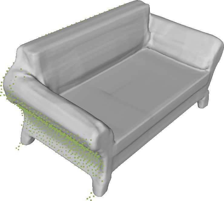
functions with arbitrary precision. Yet, the precision of
the approximation in practice is limited by the finite num-                                                  Code
                                                                    (x,y,z)                     SDF                                   SDF
ber of point samples that guide the decision boundaries and
                                                                                                            (x,y,z)
the finite capacity of the network due to restricted compute
power.                                                              (a) Single Shape DeepSDF                 (b) Coded Shape DeepSDF
   The most direct application of this approach is to train a
single deep network for a given target shape as depicted in         Figure 3: In the single-shape DeepSDF instantiation, the shape
                                                                    information is contained in the network itself whereas the coded-
Fig. 3a. Given a target shape, we prepare a set of pairs X
                                                                    shape DeepSDF, the shape information is contained in a code vec-
composed of 3D point samples and their SDF values:
                                                                    tor that is concatenated with the 3D sample location. In both cases,
                                                                    DeepSDF produces the SDF value at the 3D query location,
              X := {(x, s) : SDF (x) = s} .              (2)
                                                                        Input                     Output                         Output
We train the parameters θ of a multi-layer fully-connected                                                         Backprogate
                                                                                     Code
neural network fθ on the training set S to make fθ a good
approximator of the given SDF in the target domain Ω:

               fθ (x) ≈ SDF (x), ∀x ∈ Ω .                (3)
                                                                                                           Codes
   The training is done by minimizing the sum over losses                       (a) Auto-encoder               (b) Auto-decoder
between the predicted and real SDF values of points in X
under the following L1 loss function:                               Figure 4: Different from an auto-encoder whose latent code is
                                                                    produced by the encoder, an auto-decoder directly accepts a la-
   L(fθ (x), s) = | clamp(fθ (x), δ) − clamp(s, δ) |,    (4)        tent vector as an input. A randomly initialized latent vector is
                                                                    assigned to each data point in the beginning of training, and the la-
where clamp(x, δ) := min(δ, max(−δ, x)) introduces the              tent vectors are optimized along with the decoder weights through
parameter δ to control the distance from the surface over           standard backpropagation. During inference, decoder weights are
which we expect to maintain a metric SDF. Larger values of          fixed, and an optimal latent vector is estimated.
δ allow for fast ray-tracing since each sample gives infor-
mation of safe step sizes. Smaller values of δ can be used to
concentrate network capacity on details near the surface.           by a continuous SDF. Formally, for some shape indexed by
   To generate the 3D model shown in Fig. 3a, we use                i, fθ is now a function of a latent code zi and a query 3D
δ = 0.1 and a feed-forward network composed of eight                location x, and outputs the shape’s approximate SDF:
fully connected layers, each of them applied with dropouts.
                                                                                            fθ (zi , x) ≈ SDF i (x).                      (5)
All internal layers are 512-dimensional and have ReLU
non-linearities. The output non-linearity regressing the SDF        By conditioning the network output on a latent vector, this
value is tanh. We found training with batch-normalization           formulation allows modeling multiple SDFs with a single
[28] to be unstable and applied the weight-normalization            neural network. Given the decoding model fθ , the contin-
technique instead [46]. For training, we use the Adam op-           uous surface associated with a latent vector z is similarly
timizer [33]. Once trained, the surface is implicitly repre-        represented with the decision boundary of fθ (z, x), and the
sented as the zero iso-surface of fθ (x), which can be visu-        shape can again be discretized for visualization by, for ex-
alized through raycasting or marching cubes. Another nice           ample, raycasting or Marching Cubes.
property of this approach is that accurate normals can be              Next, we motivate the use of encoder-less training before
analytically computed by calculating the spatial derivative         introducing the ‘auto-decoder’ formulation of the shape-
∂fθ (x)/∂x via back-propogation through the network.                coded DeepSDF.
4. Learning the Latent Space of Shapes                              4.1. Motivating Encoder-less Learning
   Training a specific neural network for each shape is nei-            Auto-encoders and encoder-decoder networks are
ther feasible nor very useful. Instead, we want a model that        widely used for representation learning as their bottleneck
can represent a wide variety of shapes, discover their com-         features tend to form natural latent variable representations.
mon properties, and embed them in a low dimensional latent              Recently, in applications such as modeling depth maps
space. To this end, we introduce a latent vector z, which can       [6], faces [2], and body shapes [34] a full auto-encoder is
be thought of as encoding the desired shape, as a second in-        trained but only the decoder is retained for inference, where
put to the neural network as depicted in Fig. 3b. Concep-           they search for an optimal latent vector given some input
tually, we map this latent vector to a 3D shape represented         observation. However, since the trained encoder is unused

                                                                4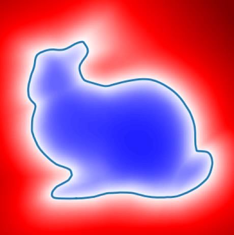
at test time, it is unclear whether using the encoder is the
most effective use of computational resources during train-
ing. This motivates us to use an auto-decoder for learning a
shape embedding without an encoder as depicted in Fig. 4.
We show that applying an auto-decoder to learn con-
tinuous SDFs leads to high quality 3D generative models.
Further, we develop a probabilistic formulation for train- Figure 5: Compared to car shapes memorized using OGN [52]
ing and testing the auto-decoder that naturally introduces (right), our models (left) preserve details and render visually pleas-
latent space regularization for improved generalization. To ing results as DeepSDF provides oriented surace normals.
the best of our knowledge, this work is the first to intro-
duce the auto-decoder learning method to the 3D learning
community. At inference time, after training and fixing θ, a shape
code zi for shape Xi can be estimated via Maximum-a-
4.2. Auto-decoder-based DeepSDF Formulation Posterior (MAP) estimation as:
To derive the auto-decoder-based shape-coded DeepSDF X 1
ẑ = arg min L(fθ (z, xj ), sj ) + 2 ||z||22 . (10)
formulation we adopt a probabilistic perspective. Given a z σ
(xj ,sj )∈X
dataset of N shapes represented with signed distance func-
N
tion SDF i i=1 , we prepare a set of K point samples and Crucially, this formulation is valid for SDF samples X
their signed distance values: of arbitrary size and distribution because the gradient of the
loss with respect to z can be computed separately for each
Xi = {(xj , sj ) : sj = SDF i (xj )} . (6)
SDF sample. This implies that DeepSDF can handle any
For an auto-decoder, as there is no encoder, each latent form of partial observations such as depth maps. This is
code zi is paired with training shape Xi . The posterior over a major advantage over the auto-encoder framework whose
shape code zi given the shape SDF samples Xi can be de- encoder expects a test input similar to the training data, e.g.
composed as: shape completion networks of [16, 58] require preparing
Q training data of partial shapes.
pθ (zi |Xi ) = p(zi ) (xj ,sj )∈Xi pθ (sj |zi ; xj ) , (7)
To incorporate the latent shape code, we stack the code
where θ parameterizes the SDF likelihood. In the latent vector and the sample location as depicted in Fig. 3b and
shape-code space, we assume the prior distribution over feed it into the same fully-connected NN described previ-
codes p(zi ) to be a zero-mean multivariate-Gaussian with ously at the input layer and additionally at the 4th layer. We
a spherical covariance σ 2 I. This prior encapsulates the no- again use the Adam optimizer [33]. The latent vector z is
tion that the shape codes should be concentrated and we initialized randomly from N (0, 0.012 ).
empirically found it was needed to infer a compact shape Note that while both VAE and the proposed auto-decoder
manifold and to help converge to good solutions. formulation share the zero-mean Gaussian prior on the la-
In the auto-decoder-based DeepSDF formulation we ex- tent codes, we found that the the stochastic nature of the
press the SDF likelihood via a deep feed-forward network VAE optimization did not lead to good training results.
fθ (zi , xj ) and, without loss of generality, assume that the
likelihood takes the form: 5. Data Preparation
pθ (sj |zi ; xj ) = exp(−L(fθ (zi , xj ), sj )) . (8) To train our continuous SDF model, we prepare the SDF
samples X (Eq. 2) for each mesh, which consists of 3D
The SDF prediction s̃j = fθ (zi , xj ) is represented using a points and their SDF values. While SDF can be computed
fully-connected network. L(s̃j , sj ) is a loss function penal- through a distance transform for any watertight shapes from
izing the deviation of the network prediction from the actual real or synthetic data, we train with synthetic objects, (e.g.
SDF value sj . One example for the cost function is the stan- ShapeNet [12]), for which we are provided complete 3D
dard L2 loss function which amounts to assuming Gaussian shape meshes. To prepare data, we start by normalizing
noise on the SDF values. In practice we use the clamped L1 each mesh to a unit sphere and sampling 500,000 spatial
cost from Eq. 4 for reasons outlined previously. points x’s: we sample more aggressively near the surface
At training time we maximize the joint log posterior over of the object as we want to capture a more detailed SDF
all training shapes with respect to the individual shape codes near the surface. For an ideal oriented watertight mesh,
{zi }Ni=1 and the network parameters θ: computing the signed distance value of x would only in-
N K volve finding the closest triangle, but we find that human
X X 1
arg min L(fθ (zi , xj ), sj ) + 2 ||zi ||22 . (9) designed meshes are commonly not watertight and con-
θ,{zi }N
i=1 i=1 j=1
σ tain undesired internal structures. To obtain the shell of a
5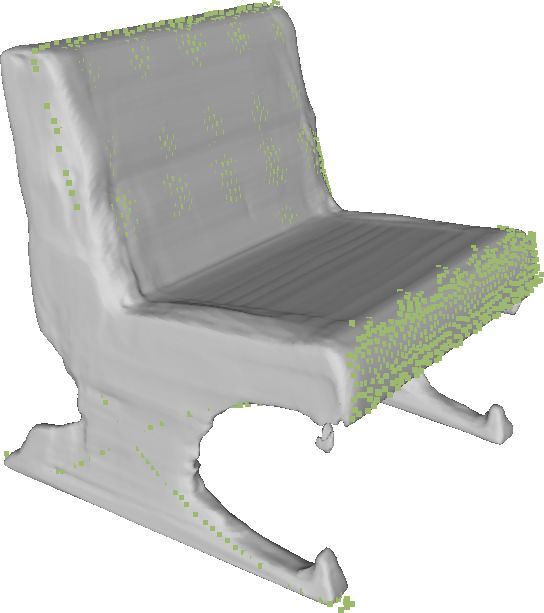
Complex          Closed      Surface          Model           Inf.        Eval.
             Method            Type       Discretization   topologies       surfaces     normals       size (GB) (s)    time (s)      tasks
             3D-EPN [16]     Voxel SDF     323 voxels         X               X             X             0.42              -          C
             OGN [52]          Octree      2563 voxels        X               X                           0.54            0.32         K
             AtlasNet        Parametric      1 patch                          X                           0.015           0.01        K, U
             -Sphere [22]      mesh
             AtlasNet        Parametric     25 patches        X                                           0.172           0.32        K, U
             -25 [22]          mesh
             DeepSDF         Continuous       none            X               X             X             0.0074          9.72      K, U, C
             (ours)             SDF

Table 1: Overview of the benchmarked methods. AtlasNet-Sphere can only describe topological-spheres, voxel/octree occupancy methods
(i.e. OGN) only provide 8 directions for normals, and AtlasNet does not provide oriented normals. Our tasks evaluated are: (K) representing
known shapes, (U) representing unknown shapes, and (C) shape completion.

mesh with proper orientation, we set up equally spaced vir-                                                 CD,         CD,        EMD,       EMD,
                                                                                       Method \metric       mean       median      mean       median
tual cameras around the object, and densely sample surface
                                                                                       OGN                  0.167      0.127       0.043      0.042
points, denoted Ps , with surface normals oriented towards                             AtlasNet-Sph.        0.210      0.185       0.046      0.045
the camera. Double sided triangles visible from both orien-                            AtlasNet-25          0.157      0.140       0.060      0.060
tations (indicating that the shape is not closed) cause prob-                          DeepSDF              0.084      0.058       0.043      0.042
lems in this case, so we discard mesh objects containing too
many of such faces. Then, for each x, we find the closest                    Table 2: Comparison for representing known shapes (K) for cars
                                                                             trained on ShapeNet. CD = Chamfer Distance (30, 000 points)
point in Ps , from which the SDF (x) can be computed. We
                                                                             multiplied by 103 , EMD = Earth Mover’s Distance (500 points).
refer readers to supplementary material for further details.

6. Results                                                                       Quantitative comparison in Table 2 shows that the pro-
    We conduct a number of experiments to show the repre-                    posed DeepSDF significantly beats OGN and AtlasNet in
sentational power of DeepSDF, both in terms of its ability                   Chamfer distance against the true shape computed with a
to describe geometric details and its generalization capabil-                large number of points (30,000). The difference in earth
ity to learn a desirable shape embedding space. Largely, we                  mover distance (EMD) is smaller because 500 points do not
propose four main experiments designed to test its ability to                well capture the additional precision. Figure 5 shows a qual-
1) represent training data, 2) use learned feature representa-               itative comparison of DeepSDF to OGN.
tion to reconstruct unseen shapes, 3) apply shape priors to
                                                                             6.2. Representing Test 3D Shapes (auto-encoding)
complete partial shapes, and 4) learn smooth and complete
shape embedding space from which we can sample new                              For encoding unknown shapes, i.e. shapes in the held-out
shapes. For all experiments we use the popular ShapeNet                      test set, DeepSDF again significantly outperforms AtlasNet
[12] dataset.                                                                on a wide variety of shape classes and metrics as shown
    We select a representative set of 3D learning approaches                 in Table 3. Note that AtlasNet performs reasonably well
to comparatively evaluate aforementioned criteria: a recent                  at classes of shapes that have mostly consistent topology
octree-based method (OGN) [52], a mesh-based method                          without holes (like planes) but struggles more on classes
(AtlasNet) [22], and a volumetric SDF-based shape comple-                    that commonly have holes, like chairs. This is shown in
tion method (3D-EPN) [16] (Table 1). These works show                        Fig. 6 where AtlasNet fails to represent the fine detail of the
state-of-the-art performance in their respective representa-                 back of the chair. Figure 7 shows more examples of detailed
tions and tasks, so we omit comparisons with the works                       reconstructions on test data from DeepSDF as well as two
that have already been compared: e.g. OGN’s octree model                     example failure cases.
outperforms regular voxel approaches, while AtlasNet com-
pares itself with various points, mesh, or voxel based meth-                 6.3. Shape Completion
ods and 3D-EPN with various completion methods.                                 A major advantage of the proposed DeepSDF approach
                                                                             for representation learning is that inference can be per-
6.1. Representing Known 3D Shapes
                                                                             formed from an arbitrary number of SDF samples. In the
   First, we evaluate the capacity of the model to represent                 DeepSDF framework, shape completion amounts to solving
known shapes, i.e. shapes that were in the training set, from                for the shape code that best explains a partial shape obser-
only a restricted-size latent code — testing the limit of ex-                vation via Eq. 10. Given the shape-code a complete shape
pressive capability of the representations.                                  can be rendered using the priors encoded in the decoder.

                                                                        6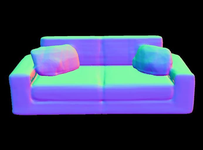
(a) Ground-truth      (b) Our Result    (c) [22]-25 patch    (d) [22]-sphere             (e) Our Result                 (f) [22]-25 patch

Figure 6: Reconstruction comparison between DeepSDF and AtlasNet [22] (with 25-plane and sphere parameterization) for test shapes.
Note that AtlasNet fails to capture the fine details of the chair, and that (f) shows holes on the surface of sofa and the plane.

Figure 7: Reconstruction of test shapes. From left to right alternating: ground truth shape and our reconstruction. The two right most
columns show failure modes of DeepSDF. These failures are likely due to lack of training data and failure of minimization convergence.

    CD, mean            chair   plane    table   lamp        sofa                                   lower is better            higher is better
    AtlasNet-Sph.       0.752   0.188    0.725   2.381      0.445              Method       CD,     CD,               Mesh     Mesh       Cos
    AtlasNet-25         0.368   0.216    0.328   1.182      0.411              \Metric      med.    mean     EMD      acc.     comp.      sim.
    DeepSDF             0.204   0.143    0.553   0.832      0.132              chair
    CD, median                                                                 3D-EPN       2.25    2.83     0.084    0.059    0.209     0.752
    AtlasNet-Sph.       0.511   0.079    0.389   2.180      0.330              DeepSDF      1.28    2.11     0.071    0.049    0.500     0.766
    AtlasNet-25         0.276   0.065    0.195   0.993      0.311              plane
    DeepSDF             0.072   0.036    0.068   0.219      0.088              3D-EPN       1.63    2.19     0.063    0.040    0.165     0.710
                                                                               DeepSDF      0.37    1.16     0.049    0.032    0.722     0.823
    EMD, mean
                                                                               sofa
    AtlasNet-Sph.       0.071   0.038    0.060   0.085      0.050
                                                                               3D-EPN       2.03    2.18     0.071    0.049    0.254     0.742
    AtlasNet-25         0.064   0.041    0.073   0.062      0.063
                                                                               DeepSDF      0.82    1.59     0.059    0.041    0.541     0.810
    DeepSDF             0.049   0.033    0.050   0.059      0.047
    Mesh acc., mean                                                        Table 4: Comparison for shape completion (C) from partial range
    AtlasNet-Sph.       0.033   0.013    0.032   0.054      0.017
                                                                           scans of unknown shapes from ShapeNet.
    AtlasNet-25         0.018   0.013    0.014   0.042      0.017
    DeepSDF             0.009   0.004    0.012   0.013      0.004

Table 3: Comparison for representing unknown shapes (U) for                surface point (along surface normal estimate). With small
various classes of ShapeNet. Mesh accuracy as defined in [47]              η we approximate the signed distance value of those points
is the minimum distance d such that 90% of generated points are            to be η and −η, respectively. We solve for Eq. 10 with
within d of the ground truth mesh. Lower is better for all metrics.        loss function of Eq. 4 using clamp value of η. Additionally,
                                                                           we incorporate free-space observations, (i.e. empty-space
                                                                           between surface and camera), by sampling points along
   We test our completion scheme using single view depth                   the freespace-direction and enforce larger-than-zero con-
observations which is a common use-case and maps well                      straints. The freespace loss is |fθ (z, xj )| if fθ (z, xj ) < 0
to our architecture without modification. Note that we cur-                and 0 otherwise.
rently require the depth observations in the canonical shape                  Given the SDF point samples and empty space points,
frame of reference.                                                        we similarly optimize the latent vector using MAP estima-
   To generate SDF point samples from the depth image ob-                  tion. Tab. 4 and Figs. (22, 9) respectively shows quantitative
servation, we sample two points for each depth observation,                and qualitative shape completion results. Compared to one
each of them located η distance away from the measured                     of the most recent completion approaches [16] using volu-

                                                                       7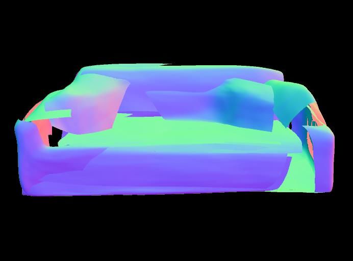
(a) Input Depth              (b) Completion (ours)        (c) Second View (ours)       (d) Ground truth          (e) 3D-EPN

Figure 8: For a given depth image visualized as a green point cloud, we show a comparison of shape completions from our DeepSDF
approach against the true shape and 3D-EPN.

                                                                           7. Conclusion & Future Work
                                                                               DeepSDF significantly outperforms the applicable
                                                                           benchmarked methods across shape representation and
  (a) Noisy Input Point Cloud          (b) Shape Completion                completion tasks and simultaneously addresses the goals
                                                                           of representing complex topologies, closed surfaces, while
Figure 9: Demonstration of DeepSDF shape completion from a                 providing high quality surface normals of the shape. How-
partial noisy point cloud. Input here is generated by perturbing the       ever, while point-wise forward sampling of a shape’s SDF is
3D point cloud positions generated by the ground truth depth map           efficient, shape completion (auto-decoding) takes consider-
by 3% of the plane length. We provide a comprehensive analysis             ably more time during inference due to the need for explicit
of robustness to noise in the supplementary material.                      optimization over the latent vector. We look to increase per-
                                                                           formance by replacing ADAM optimization with more ef-
                                                                           ficient Gauss-Newton or similar methods that make use of
metric shape representation, our continuous SDF approach                   the analytic derivatives of the model.
produces more visually pleasing and accurate shape recon-
structions. While a few recent shape completion methods                       DeepSDF models enable representation of more com-
were presented [24, 55], we could not find the code to run                 plex shapes without discretization errors with significantly
the comparisons, and their underlying 3D representation is                 less memory than previous state-of-the-art results as shown
voxel grid which we extensively compare against.                           in Table 1, demonstrating an exciting route ahead for 3D
                                                                           shape learning. The clear ability to produce quality latent
6.4. Latent Space Shape Interpolation                                      shape space interpolation opens the door to reconstruction
                                                                           algorithms operating over scenes built up of such efficient
   To show that our learned shape embedding is complete                    encodings. However, DeepSDF currently assumes models
and continuous, we render the results of the decoder when                  are in a canonical pose and as such completion in-the-wild
a pair of shapes are interpolated in the latent vector space               requires explicit optimization over a SE(3) transformation
(Fig. 1). The results suggests that the embedded continuous                space increasing inference time. Finally, to represent the
SDF’s are of meaningful shapes and that our representation                 true space-of-possible-scenes including dynamics and tex-
extracts common interpretable shape features, such as the                  tures in a single embedding remains a major challenge, one
arms of a chair, that interpolate linearly in the latent space.            which we continue to explore.

                                                                       8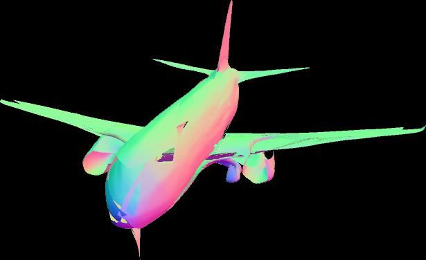
Supplementary
A. Overview                                                                               6            raw perturbed depth image
    This supplementary material provides quantitative and                                              completion, mean
                                                                                          5            completion, median

                                                                       Chamfer Distance
qualitative experimental results along with extended tech-
nical details that are supplementary to the main paper. We                                4
first describe the shape completion experiment with noisy
                                                                                          3
depth maps using DeepSDF (Sec. B). We then discuss ar-
chitecture details (Sec. C) along with experiments exploring                              2
characteristics and tradeoffs of the DeepSDF design deci-
sions (Sec. D). In Sec. E we compare auto-decoders with                                   1
variational and standard auto-encoders. Further, additional                               0
details on data preparation (Sec. F), training (Sec. G), the
                                                                                              0.00        0.01       0.02      0.03     0.04      0.05
auto-decoder learning scheme (Sec. H), and quantitative                                              α , std. dev of inverse-depth Gaussian noise
evaluations (Sec. I) are presented, and finally in Sec. J we
provide additional quantitative and qualitative results.            Figure 10: Chamfer distance (multiplied by 103 ) as a function
                                                                    of α, the standard deviation of inverse-depth Gaussian noise as
B. Shape Completion from Noisy Depth Maps                           shown in Eq. 11, for shape completions on planes from ShapeNet.
                                                                    Green line describes Chamfer distance between the perturbed
   We test the robustness of our shape completion method            depth points and original depth points, which shows the superlin-
by using noisy depth maps as input. Specifically, we                ear increase with increased noise. Blue and orange show respec-
demonstrate the ability to complete shapes given partial            tively the mean and median of the shape completion’s Chamfer
noisy point clouds obtained from consumer depth cameras.            distance (over a dataset of 85 plane completions) relative to the
Following [25], we simulate the noise distribution of typi-         ground truth mesh which deteriorates approximately linearly with
cal structure depth sensors, including Kinect V1 by adding          increasing standard deviation of noise. The same DeepSDF model
                                                                    was used for inference, the only difference is in the noise of the
zero-mean Guassian noise to the inverse depth representa-
                                                                    single depth image provided from which to perform shape com-
tion of a ground truth input depth image:                           pletion. Example qualitative resuls are shown in Fig. 11.
                                 1
               Dnoise =                      ,          (11)
                          (1/D) + N (0, α2 )
                                                                    posed of 8 fully connected layers each of which are applied
where α is standard deviation of the normal distribution.           with weight-normalization, and each intermediate vectors
   For the experiment, we synthetically generate noisy              are processed with RELU activation and 0.2 dropout ex-
depth maps from the ShapeNet [12] plane models using the            cept for the final layer. A skip connection is included at the
same benchmark test set of Dai et al. [16] used in the main         fourth layer.
paper. We perturb the depth values using standard deviation
α of 0.01, 0.02, 0.03, and 0.05. Given that the target shapes       D. DeepSDF Network Design Decisions
are normalized to a unit sphere, one can observe that the              In this section, we study system parameter decisions that
inserted noise level is significant (Fig. 10).                      affect the accuracy of SDF regression, thereby providing
   The shape completion results with respect to added               insight on the tradeoffs and scalability of the proposed al-
Guassian noise on the input synthetic depth maps are shown          gorithm.
in Fig. 11. The Chamfer distance of the inferred shape ver-
sus the ground truth shape deteriorates approximately lin-          D.1. Effect of Network Depth on Regression Accu-
early with increasing standard deviation of the noise. Com-               racy
pared to the Chamfer distance between raw perturbed point
                                                                        In this experiment we test how the expressive capabil-
cloud and ground truth depth map, which increases super-
                                                                    ity of DeepSDF varies as a function of the number of lay-
linearly with increasing noise level (Fig. 11), the shape
                                                                    ers. Theoretically, an infinitely deep feed-forward network
completion quality using DeepSDF degrades much slower,
                                                                    should be able to memorize the training data with arbitrary
implying that the shape priors encoded in the network play
                                                                    precision, but in practice this is not true due to finite com-
an important role regularizing the shape reconstruction.
                                                                    pute power and the vanishing gradient problem, which lim-
C. Network Architecture                                             its the depth of the network.
                                                                        We conduct an experiment where we let DeepSDF mem-
    Fig. 13 depicts the overall architecture of DeepSDF. For        orize SDFs of 500 chairs and inspect the training loss with
all experiments in the main paper we used a network com-            varying number of layers. As described in Fig. 13, we find

                                                                9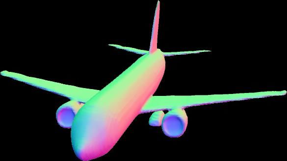
(a) No noise                (b) α = 0.01                 (c) α = 0.02                   (d) α = 0.03               (e) α = 0.05

Figure 11: Shape completion results obtained from the partial and noisy input depth maps shown below. Input point clouds are overlaid
on each completion to illustrate the scale of noise in the input.

           (a) No noise             (b) α = 0.01               (c) α = 0.02               (d) α = 0.03                 (e) α = 0.05

Figure 12: Visualization of partial and noisy point-clouds used to test shape completion with DeepSDF. Here, α is the standard deviation
of Gaussian noise in Eq. 11. Corresponding completion results are shown above.

                 259         512          512           512          512           512           512          512

Latent Vector                                                                                                                1            1
                       FC           FC            FC           FC            FC           FC           FC            FC            TH

       (x,y,z)

Figure 13: DeepSDF architecture used for experiments. Boxes represent vectors while arrows represent operations. The feed-forward
network is composed of 8 fully connected layers, denoted as “FC” on the diagram. We used 256 and 128 dimensional latent vectors for
reconstruction and shape completion experiments, respectively. The latent vector is concatenated, denoted “+”, with the xyz query, making
259 length vector, and is given as input to the first layer. We find that inserting the latent vector again to the middle layers significantly
improves the learning, denoted as dotted arrow in the diagram: the 259 vector is concatenated with the output of fourth fully connected
layer to make a 512 vector. Final SDF value is obtained with hypberbolic tangent non-linear activation denoted as “TH”.

that applying the input vector (latent vector + xyz query)                 with latent vector skip connections. Compared to the archi-
both to the first and a middle layer improves training. In-                tecture we used for the main experiments (8 FC layers), a
spired by this, we split the experiment into two cases: 1)                 network with 16 layers produces significantly smaller train-
train a regular network without skip connections, 2) train a               ing error, suggesting a possibility of using a deeper network
network by concatenating the input vector to every 4 layers                for higher precision in some application scenarios. Further,
(e.g. for 12 layer network the input vector will be concate-               we observe that the test error quickly decrease from four-
nated to the 4th, and 8th intermediate feature vectors).                   layer architecture (9.7) to eight layer one (5.7) and subse-
                                                                           quently plateaued for deeper architectures. However, this
   Experiment results in Fig. 14 shows that the DeepSDF                    does not suggest conclusive results on generalization, as we
architecture without skip connections gets quickly saturated               used the same number of small training data for all archi-
at 4 layers while the error keeps decreasing when trained

                                                                     10
Training Loss by Network Size
8
Without Skip
7 With Skip
Chamfer Distance (30,000 points)
0.10
6
Training SDF Loss (1e-3)
0.09
5
0.08
4 Our Used Model
0.07
3
2 0.06 mean
median
1 0.05
0.2 0.4 0.6 0.8 1.0
0 δ , Truncation distance
2 4 6 8 10 12 14 16 18 20
Number of FC Layers Figure 15: Chamfer distance (multiplied by 103 ) as a function of
δ, the truncation distance, for representing a known small dataset
Figure 14: Regression accuracy (measured by the SDF loss used
of 100 cars from ShapeNet dataset [12]. All models were trained
in training) as a function of network depth. Without skip con-
on the same set of SDF samples from these 100 cars. There is
nections, we observe a plateau in training loss past 4 layers. With
a moderate reduction in the accuracy of the surface, as measured
skip connections, training loss continues to decrease although with
by the increasing Chamfer distance, as the truncation distance is
diminishing returns past 12 layers. The model size chosen for
increased between 0.05 and 1.0. The bend in the curve at δ = 0.3
all other experiments, 8 layers, provides a good tradeoff between
is just expected to be due to the stochasticity inherent in training.
speed and accuracy.
Note that (a) due to the tanh() activation in the final layer, 1.0
is the maximum value the model can predict, and (b) the plot is
dependent on the distribution of the samples used during training.
tectures even though a network with more number of pa-
rameters tends to require higher volume of data to avoid E. Comparison with Variational and Standard
overfitting.
Auto-encoders on MNIST
To compare different approaches of learning a latent
D.2. Effect of Truncation Distance on Regression code-space for a given datum, we use the MNIST dataset
Accuracy and compare the variational auto encoder (VAE), the stan-
dard bottleneck auto encoder (AE), and the proposed auto
We study the effect of the truncation distance (δ from decoder (AD). As the reconstruction error we use the stan-
Eq. 4 of the manuscript) on the regression accuracy of the dard binary cross-entropy and match the model architec-
model. The truncation distance controls the extent from the tures such that the decoders of the different approaches have
surface over which we expect the network to learn a met- exactly the same structure and hence theoretical capacity.
ric SDF. Fig. 15 plots the Chamfer distance as a function of We show all evaluations for different latent code-space di-
truncation distance. We observe a moderate decrease in the mensions of 2D, 5D and 15D.
accuracy of the surface representation as the truncation dis- For 2D codes the latent spaces learned by the different
tance is increased. A hypothesis for an explanation is that methods are visualized in Fig. 16. All code spaces can rea-
it becomes more difficult to approximate a larger truncation sonably represent the different digits. The AD latent space
region (a strictly larger domain of the function) to the same seems more condensed than the ones from VAE and AE.
absolute accuracy as a smaller truncation region. The ben- For the optimization-based encoding approach we initialize
efit, however, of larger truncation regions is that there is a codes randomly. We show visualizations of such random
larger region over which the metric SDF is maintained – in samples in Fig. 17. Note that samples from the AD- and
our application this reduces raycasting time, and there are VAE-learned latent code spaces mostly look like real digits,
other applications as well, such as physics simulation and showing their ability to generate realistic digit images.
robot motion planning for which a larger SDF of shapes We also compare the train and test reconstruction errors
may be valuable. We chose a δ value of 0.01 for all exper- for the different methods in Fig. 18. For VAE and AE
iments presented in the manuscript, which provides a good we show both the reconstruction error obtained using the
tradeoff between raycasting speed and surface accuracy. learned encoder and obtained via code optimization using
11(a) Auto Encoder (AE) (b) Variational Auto Encoder (VAE) (c) Auto Decoder (AD)
Figure 16: Comparison of the 2D latent code-space learned by the different methods. Note that large portion of the regular auto-encoder’s
(AE) latent embedding space contains images that do not look like digits. In contrast, both VAE and AD generate smooth and complete
latent space without outstanding artifacts. Best viewed digitally.
While the reconstructions from “VAE decode“ are, for the
most part, qualitatively close to the original, AD’s recon-
structions more closely resemble the actual digit of the test
data. Qualitatively, AD is on par with reconstructions from
end-to-end-trained VAE and AE.
F. Data Preparation Details
For data preparation, we are given a mesh of a shape
to sample spatial points and their SDF values. We begin
(a) AD (b) VAE (c) AE by normalizing each shape so that the shape model fits into
a unit sphere with some margin (in practice fit to sphere
Figure 17: Visualization of random samples from the latent 2D radius of 1/1.03). Then, we virtually render the mesh from
(top), 5D (middle), and 15D (bottom) code space on MNIST. Note 100 virtual cameras regularly sampled on the surface of the
that the sampling from regular auto-encoder (AE) suffers from ar- unit sphere. Then, we gather the surface points by back-
tifacts. Best viewed digitally. projecting the depth pixels from the virtual renderings, and
the points’ normals are assigned from the triangle to which
it belongs. Triangle surface orientations are set such that
the learned decoder only (denoted “(V)AE decode”). The they are towards the camera. When a triangle is visible from
test error for VAE and AE are consistently minimized for both orientations, however, the given mesh is not watertight,
all latent code dimensions. “AE decode ” diverges in all making true SDF values hard to calculate, so we discard a
cases hinting at a learned latent space that is poorly suited mesh with more than 2% of its triangles being double-sided.
for optimization-based decoding. Optimizing latent codes For a valid mesh, we construct a KD-tree for the oriented
using the VAE encoder seems to work better for higher di- surface points.
mensional codes. The proposed AD approach works well in As stated in the main paper, it is important that we sam-
all tested code space dimensions. Although “VAE decode” ple more aggressively near the surface of the mesh as we
has slightly lower test error than AD in 15 dimensions, qual- want to accurately model the zero-crossings. Specifically,
itatively the AD’s reconstructions are better as we discuss we sample around 250,000 points randomly on the surface
next. of the mesh, weighted by triangle areas. Then, we perturb
In Fig. 19 we show example reconstructions from the each surface point along all xyz axes with mean-zero Gaus-
test dataset. When using the learned encoders VAE and sian noise with variance 0.0025 and 0.00025 to generate
AE produce qualitatively good reconstructions. When using two spatial samples per surface point. For around 25,000
optimization-based encoding “AE decode” performs poorly points we uniformly sample within the unit sphere. For each
indicating that the latent space has many bad local minima. collected spatial samples, we find the nearest surface point
12(a) 2D (b) 5D (c) 15D
Figure 18: Train and test error for different dimensions of the latent code for the different approaches.
(a) AD (b) VAE (c) VAE decode (d) AE (e) AE decode
Figure 19: Reconstructions for 2D (top), 5D (middle), and 15D (bottom) code space on MNIST. For each of the different dimensions we
plot the given test MNIST image and the reconstruction given the inferred latent code.
N
from the KD-tree, measure the distance, and decide the sign tion SDF i i=1 , we prepare a set of K point samples and
from the dot product between the normal and their vector their signed distance values:
difference.
Xi = {(xj , sj ) : sj = SDF i (xj )} . (12)
G. Training and Testing Details The SDF values can be computed from mesh inputs as de-
tailed in the main paper.
For training, we find it is important to initialize the latent For an auto-decoder, as there is no encoder, each la-
vectors quite small, so that similar shapes do not diverge tent code zi is paired with training shape data Xi and
in the latent vector space – we used N (0, 0.012 ). Another randomly initialized from a zero-mean Gaussian. We use
crucial point is balancing the positive and negative samples N (0, 0.0012 ). The latent vectors {zi }N i=1 are then jointly
both for training and testing: for each batch used for gradi- optimized during training along with the decoder parame-
ent descent, we set half of the SDF point samples positive ters θ.
and the other half negative. We assume that each shape in the given dataset X =
Learning rate for the decoder parameters was set to be {Xi }Ni=1 follows the joint distribution of shapes:
1e-5 * B, where B is number of shapes in one batch. For
each shape in a batch we subsampled 16384 SDF samples. pθ (Xi , zi ) = pθ (Xi |zi )p(zi ) , (13)
Learning rate for the latent vectors was set to be 1e-3. Also, where θ parameterizes the data likelihood. For a given θ a
we set the regularization parameter σ = 10−2 . We trained shape code zi can be estimated via Maximum-a-Posterior
our models on 8 Nvidia GPUs approximately for 8 hours (MAP) estimation:
for 1000 epochs. For reconstruction experiments the latent
vector size was set to be 256, and for the shape completion ẑi = arg max pθ (zi |Xi ) = arg max log pθ (zi |Xi ) . (14)
zi zi
task we used models with 128 dimensional latent vectors.
We estimate θ as the parameters that maximizes the poste-
H. Full Derivation of Auto-decoder-based rior across all shapes:
X
DeepSDF Formulation θ̂ = arg max max log pθ (zi |Xi ) (15)
θ zi
Xi ∈X
To derive the auto-decoder-based shape-coded DeepSDF X
formulation we adopt a probabilistic perspective. Given a = arg max max(log pθ (Xi |zi ) + log p(zi )) ,
θ zi
dataset of N shapes represented with signed distance func- Xi ∈X
13where the second equality follows from Bayes Law. Cubes [35] with 5123 resolution. Note that while this was
For each shape Xi defined via point and SDF samples done for quantitative evaluation as a mesh, many of the
(xj , sj ) as defined in Eq. 12 we make a conditional inde- qualitative renderings are instead produced by raycasting
pendence assumption given the code zi to arrive at the de- directly against the continuous SDF model, which can avoid
composition of the posterior pθ (Xi |zi ): some of the artifacts produced by Marching Cubes at fi-
Y nite resolution. For all experiments in representing known
pθ (Xi |zi ) = pθ (sj |zi ; xj ) . (16) or unknown shapes, DeepSDF was trained on ShapeNet
(xj ,sj )∈Xi v2, while all shape completion experiments were trained
Note that the individual SDF likelihoods pθ (sj |zi ; xj ) are on ShapeNet v1, to match 3D-EPN. Additional DeepSDF
parameterized by the sampling location xj . training details are provided in Sec. G.
To derive the proposed auto-decoder-based DeepSDF
approach we express the SDF likelihood via a deep feed-
forward network fθ (zi , xj ) and, without loss of generality, I.1.2 OGN
assume that the likelihood takes the form:
For OGN we trained the provided decoder model
pθ (sj |zi ; xj ) = exp(−L(fθ (zi , xj ), sj )) . (17) (“shape from id”) for 300,000 steps on the same train set
The SDF prediction s̃j = fθ (zi , xj ) is represented using of cars used for DeepSDF. To compute the point-based
a fully-connected network and L(s̃j , sj ) is a loss function metrics, we took the pair of both the groundtruth 256-
penalizing the deviation of the network prediction from the voxel training data provided by the authors, and the gen-
actual SDF value sj . One example for the cost function is erated 256-voxel output, and converted both of these into
the standard L2 loss function which amounts to assuming point clouds of only the surface voxels, with one point for
Gaussian noise on the SDF values. In practice we use the each of the voxels’ centers. Specifically, surface voxels
clamped L1 cost introduced in the main manuscript. were defined as voxels which have at least one of 6 di-
In the latent shape-code space, we assume the prior dis- rect (non-diagonal) voxel neighbors unoccupied. A typi-
tribution over codes p(zi ) to be a zero-mean multivariate- cal number of vertices in the resulting point clouds is ap-
Gaussian with a spherical covariance σ 2 I. Note that other proximately 80,000, and the points used for evaluation are
more complex priors could be assumed. This leads to the fi- randomly sampled from these sets. Additionally, OGN was
nal cost function via Eq. 15 which we jointly minimize with trained based on ShapeNet v1, while AtlasNet was trained
respect to the network parameters θ and the shape codes on ShapeNet v2. To adjust for the scale difference, we con-
{zi }N verted OGN point clouds into ShapeNet v2 scale for each
i=1 :
model.
N K
X X 1
arg min L(fθ (zi , xj ), sj ) + 2 ||zi ||22 . (18)
θ,{zi }N
i=1 i=1 j=1
σ
I.1.3 AtlasNet
At inference time, we are given SDF point samples X of
one underlying shape to estimate the latent code z describ- Since the provided pretrained AtlasNet models were trained
ing the shape. Using the MAP formulation from Eq. 14 with multi-class, we instead trained separate AtlasNet models for
fixed network parameters θ we arrive at: each evaluation. Each model was trained with the avail-
able code by the authors with all default parameters, except
X 1
ẑ = arg min L(fθ (z, xj ), sj ) + 2 ||z||22 , (19) for the specification of class for each model and matching
z σ train/test splits with those used for DeepSDF. The quality of
(xj ,sj )∈X
the models produced from these trainings appear compara-
where σ12 can be used to balance the reconstruction and reg- ble to those in the original paper.
ularization term. For additional comments and insights as
Of note, we realized that AtlasNet’s own computation
well as the practical implementation of the network and its
of its training and evaluation metric, Chamfer distance, had
training refer to the main manuscript.
the limitation that only the vertices of the generated mesh
I. Details on Quantitative Evaluations were used for the evaluation. This leaves the triangles of
the mesh unconstrained in that they can connect across what
I.1. Preparation for Benchmarked Methods are supposed to be holes in the shape, and this would not be
reflected in the metric. Our evaluation of meshes produced
I.1.1 DeepSDF
by AtlasNet instead samples evenly from the mesh surface,
For quantitative evaluations we converted the DeepSDF i.e. each triangle in the mesh is weighted by its surface area,
model for a given shape into a mesh by using Marching and points are sampled from the triangle faces.
14I.1.4 3D-EPN schemes [5] for speed during training, we compute the met-
ric accurately for evaluation using a more modest number
We used the provided shape completion inference results for of point samples (500) using [18].
3D-EPN, which is in voxelized distance function format.
In practice the intuitive, important difference between
We subsequently extracted the isosurface using MATLAB
the Chamfer and Earth Mover’s metrics is that the Earth
as described in the paper to obtain the final mesh.
Mover’s metric more favors distributions of points that are
I.2. Metrics similarly evenly distributed as the ground truth distribution.
A low Chamfer distance may be achieved by assigning just
The first two metrics, Chamfer and Earth Mover’s, are one point in S2 to a cluster of points in S1 , but to achieve
easily applicable to points, meshes (by sampling points a low Earth Mover’s distance, each cluster of points in S1
from the surface) and voxels (by sampling surface voxels requires a comparably sized cluster of points in S2 .
and treating their centers as points). When meshes are
available, we also can compute metrics suited particularly Mesh accuracy, as defined in [47], is the minimum
for meshes: mesh accuracy, mesh completion, and mesh distance d such that 90% of generated points are within d
cosine similarity. of the ground truth mesh. We used 1,000 points sampled
evenly from the generated mesh surface, and computed the
Chamfer distance is a popular metric for evaluating minimum distances to the full ground truth mesh. To clar-
shapes, perhaps due to its simplicity [19]. Given two point ify, the distance is computed to the closest point on any face
sets S1 and S2 , the metric is simply the sum of the nearest- of the mesh, not just the vertices. Note that unlike Chamfer
neighbor distances for each point to the nearest point in the and Earth Mover’s metrics which require sampling of points
other point set. from both meshes, with this metric the entire mesh for the
X X ground truth is used – accordingly this metric has lower
dCD (S1 , S2 ) = min ||x − y||22 + min ||x − y||22 variance than for example Chamfer distance computed with
y∈S2 x∈S1
x∈S1 y∈S2
only 1,000 points from each mesh. Note also that mesh
Note that while sometimes the metric is only defined accuracy does not measure how complete the generated
one-way (i.e., just x∈S1 min||x − y||22 ) and this is not
P mesh is – a low (good) mesh accuracy can be achieved
y∈S2 by only generating one small portion of the ground truth
symmetric, the sum of both directions, as defined above, is mesh, ignoring the rest. Accordingly, it is ideal to pair
symmetric: dCD (S1 , S2 ) = dCD (S2 , S1 ). Note also that mesh accuracy with the following metric, mesh completion.
the metric is not technically a valid distance function since
it does not satisfy the triangle inequality, but is commonly Mesh completion, also as defined in [47], is the fraction
used as a psuedo distance function [19]. In all of our of points sampled from the ground truth mesh that are
experiments we report the Chamfer distance for 30,000 within some distance ∆ (a parameter of the metric) to the
points for both |S1 | and |S2 |, which can be efficiently generated mesh. We used ∆ = 0.01, which well measured
computed by use of a KD-tree, and akin to prior work the differences in mesh completion between the different
[22] we normalize by the number of points: we report methods. With this metric the full generated mesh is used,
dCD (S1 ,S2 )
30,000 . and points (we used 1,000) are sampled from the ground
truth mesh (mesh accuracy is vice versa). Ideal mesh
Earth Mover’s distance [45], also known as the Wasser- completion is 1.0, minimum is 0.0.
stein distance, is another popular metric for measuring the
difference between two discrete distributions. Unlike the Mesh cosine similarity is a metric we introduce to mea-
Chamfer distance, which does not require any constraints sure the accuracy of mesh normals. We define the metric
on the correspondences between evaluated points, for the as the mean cosine similarity between the normals of points
Earth Mover’s distance a bijection φ : S1 → S2 , i.e. a sampled from the ground truth mesh, and the normals of the
one-to-one correspondence, is formed. Formally, for two nearest faces of the generated mesh. More precisely, given
point sets S1 and S2 of equal size |S1 | = |S2 |, the metric is the generated mesh Mgen and a set of points with normals
defined via the optimal bijection [19]: Sgt sampled from the ground truth mesh, for each point xi
in Sgt we look up the closest face Fi in Mgen , and then
X compute the average cosine similarity between the normals
dEM D (S1 , S2 ) = min ||x − φ(x)||2
φ:S1 →S2 associated with xi and Fi ,
x∈S1
Although the metric is commonly approximated in the 1 X
Cos. sim(Mgen , Sgt ) = n̂Fi · n̂xi ,
deep learning literature [19] by distributed approximation |Sgt |
xi ∈Sgt
15You can also read