Does SUSY have friends? A new approach for LHC event analysis - Inspire HEP
←
→
Page content transcription
If your browser does not render page correctly, please read the page content below
Published for SISSA by       Springer
                                                                  Received: January    23,   2020
                                                                  Revised: December    23,   2020
                                                                 Accepted: December    24,   2020
                                                                 Published: February   18,   2021

Does SUSY have friends? A new approach for LHC
event analysis

                                                                                                    JHEP02(2021)160
Anna Mullin,a Stuart Nicholls,a Holly Pacey,b Michael Parker,b Martin Whitea
and Sarah Williamsb
a
  ARC Center of Excellence for Particle Physics at the Terascale & CSSM,
  Department of Physics, University of Adelaide, Adelaide, Australia
b
  Cavendish Laboratory,
  Madingley Road, Cambridge CB3 0HE, U.K.
    E-mail: anna.mullin@adelaide.edu.au, stuart.nicholls@adelaide.edu.au,
    hp341@cam.ac.uk, parker@hep.phy.cam.ac.uk,
    martin.white@adelaide.edu.au, sarah.louise.williams@cern.ch

Abstract: We present a novel technique for the analysis of proton-proton collision events
from the ATLAS and CMS experiments at the Large Hadron Collider. For a given final state
and choice of kinematic variables, we build a graph network in which the individual events
appear as weighted nodes, with edges between events defined by their distance in kinematic
space. We then show that it is possible to calculate local metrics of the network that serve
as event-by-event variables for separating signal and background processes, and we evaluate
these for a number of different networks that are derived from different distance metrics.
Using a supersymmetric electroweakino and stop production as examples, we construct
prototype analyses that take account of the fact that the number of simulated Monte
Carlo events used in an LHC analysis may differ from the number of events expected in the
LHC dataset, allowing an accurate background estimate for a particle search at the LHC
to be derived. For the electroweakino example, we show that the use of network variables
outperforms both cut-and-count analyses that use the original variables and a boosted
decision tree trained on the original variables. The stop example, deliberately chosen to be
difficult to exclude due its kinematic similarity with the top background, demonstrates that
network variables are not automatically sensitive to BSM physics. Nevertheless, we identify
local network metrics that show promise if their robustness under certain assumptions of
node-weighted networks can be confirmed.

Keywords: Supersymmetry Phenomenology

ArXiv ePrint: 1912.10625

Open Access, c The Authors.
                                                    https://doi.org/10.1007/JHEP02(2021)160
Article funded by SCOAP3 .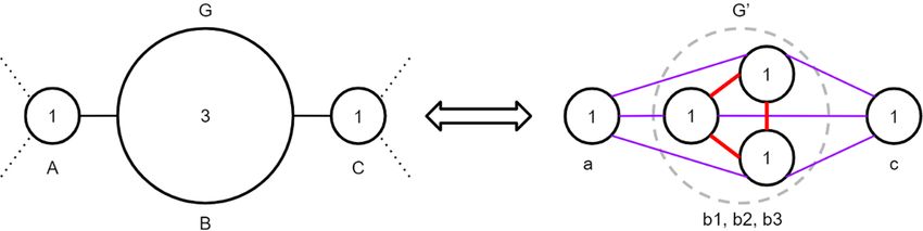
Contents

1 Introduction                                                                           1

2 Network analysis                                                                       3
  2.1 Overview                                                                           3
  2.2 Network metrics                                                                    5

3 Simulated signal and background event samples                                          9

                                                                                              JHEP02(2021)160
4 Case study 1: the search for electroweakinos                                          11
  4.1 Electroweakino analysis design                                                    11
  4.2 Results of realistic electroweakino exclusion test                                17

5 Case study 2: the search for stop quarks                                              19
  5.1 Stop analysis design                                                              19

6 Discussion                                                                            21

7 Conclusions                                                                           27

A Justifying the robustness of n.s.i. network metrics                                   28
  A.1 Empirical tests                                                                   28
  A.2 Theoretical considerations                                                        30
       A.2.1 Accuracy of n.s.i. assumptions in this context                             30
       A.2.2 Justifying the choice of network metrics used                              32

1   Introduction
The search for physics beyond the Standard Model (BSM) at the Large Hadron Collider
(LHC) has thus far not produced any significant evidence for new phenomena, despite many
analyses targeting the new particles that arise in a variety of Standard Model extensions.
What this means precisely for the landscape of BSM physics models is unclear, since null
results are difficult to interpret even within one BSM theory due to the large parameter
space and the complexity of the particle spectra predictions.
     In fact, there are specific cases where the LHC results are known to provide no con-
straint in general. For example, a recent global fit of the electroweakino sector of the
Minimal Supersymmetric Standard Model (MSSM) [1] demonstrated that there is no sig-
nificant general exclusion on any range of electroweakino masses. The fact that the weakly-
produced supersymmetric signal is very low rate compared to the dominant Standard Model
background processes means that searches need to be very heavily optimised for specific
scenarios in order to provide any sensitivity for discovery. This reduces sensitivity to a

                                          –1–
large range of models that do not resemble the simplified models used for optimisation [2].
Similar arguments should apply to other sectors of supersymmetry (SUSY), and previous
global fits have indeed found ample parameter space for light coloured sparticles once their
decays are allowed to be more complex than those encountered in simplified models [3–7].
     There is clearly a strong motivation to revisit particle search techniques, and find
new ways of extracting small signals from the LHC data. All LHC analyses start from a
knowledge of the reconstructed objects in each event, and their reconstructed energies and
momenta. These are the attributes of the event, and one typically searches for functions of
the four-momenta of the final state particles that, within a given final state, provide effective
discrimination between the signal being searched for, and the dominant SM background

                                                                                                    JHEP02(2021)160
processes. One can then place a series of selections on these kinematic variables (or perform
a machine-learning based classification) in order to find regions of the data that should
contain a significant excess of signal events.
     In this paper, we propose a novel approach for analysing LHC events that examines the
connections between events to define new event-by-event attributes which can be analysed
in the usual way. Given a set of kinematic variables, the LHC collision events form a
topological structure in kinematic space, and one should expect there to be significant
differences between the topological structures predicted for SM events, and those predicted
for signal events. Motivated by studies of galaxy topology [8], we build a series of network
graphs from simulated LHC events, each of which uses a particular distance metric to
define “friendship” between events based on their proximity in a chosen space of kinematic
variables. For example, considering only the missing energy values reconstructed for each
event, the SM events will cluster in a group at lower missing energy, each having many
“friends” close by, while SUSY events can be expected to be few and far from the main part
of the distribution, giving a small number of “friends” when viewed as part of a network.
In defining friendship in a larger space of kinematic variables, we perform an appropriate
scaling of the variables and use them to calculate a distance metric. This is then used
to define connections between events that are closer than some distance l, which is a free
parameter. A variety of local network metrics can then be calculated for each network,
which serve to define new event-by-event attributes that can be used to discriminate rare
signals from their dominant SM backgrounds. The analysis is complicated by the need to
use local metrics that are invariant under the reweighting of the network nodes (to cope
with arbitrary integrated luminosities of simulated MC events with non-trivial individual
weights), and we provide a detailed solution that is applied to two supersymmetric examples
based on stop quark or electroweakino production.
     We note that graph networks have recently been used for a variety of applications in
particle physics (usually in the context of deep learning studies), including jet tagging [9–
12], modelling kinematics within an event for classification [13, 14], reconstructing tracks
in silicon detectors [15], pile-up subtraction at the LHC [16], investigating multiparticle
correlators [17], and particle reconstruction in calorimeters [18]. A recent work that in-
vestigates the relationship between events is the exploration of the earth-moving distance
metric presented in refs. [19, 20], although this did not involve building a network based
on the metric. Our work is distinguished by the fact that it builds a graph network across

                                             –2–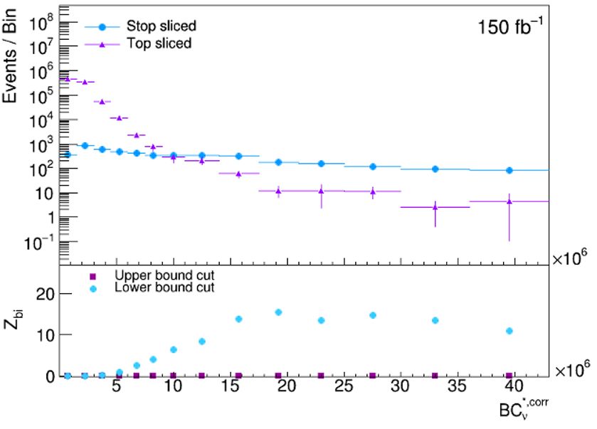
proton-proton collision events, and we investigate a number of different distance metrics,
and local network metrics, for separating events.
This paper is structured as follows. In section 2, we provide a brief review of the rele-
vant network analysis concepts, and present our method for defining connections between
LHC events. We develop our electroweakino case study in section 4, and our stop quark
example in section 5. A discussion of various aspects of the future applicability of our
technique is contained in section 6. Finally, we present our conclusions in section 7.
2 Network analysis
JHEP02(2021)160
2.1 Overview
A network is a mathematical data structure that is comprised of nodes connected by either
directed or undirected edges. In the following, we will consider finite, undirected graph
networks denoted by G = (N , E), where N is the set of nodes, and E ⊆ {{i, j} : i 6= j ∈ N }
is the edge list. Graphs can be described in a number of ways, and for large graphs
a particularly convenient form is the adjacency matrix which has the list of nodes as the
rows and columns. Connected nodes have a 1 in the relevant adjacency matrix entry, whilst
disconnected nodes have a 0. We may write this as A = (aij )i,j∈N , where aij ∈ {0, 1} and
aij = 1 iff {i, j} ∈ E, and we note that the adjacency matrix will be symmetric in our
case. The neighbours of a node ν ∈ N are those that are linked to the node by an edge,
defined via:
Nν = {i ∈ N : aiν = 1} (2.1)
These are also referred to as the members of ν’s punctured neighbourhood. We can define
an extended adjacency matrix A+ = (a+ ij )i,j∈N = A + I with:
a+
ij = aij + δij (2.2)
where I is the identity matrix, and δij is the Kronecker delta symbol. This then allows us
to define the unpunctured neighbourhood of ν as the set of nodes which includes both the
neighbours of ν, and ν itself:
n o
N + = i ∈ N : a+
iν = 1 = Nν ∪ {ν} (2.3)
In our analysis, we will define the adjacency matrix for LHC events by defining a
distance between events in the space of kinematic variables that are measured for each
event. Assuming some distance dij between the nodes in this space of variables, one can
then define the adjacency matrix via:
1, if dij ≤ l,
aij = (2.4)
0, otherwise,
where l is a free parameter known as the linking length. This prescription clearly leaves
many choices open for how to proceed, including the choice of kinematic variables, the
choice of distance metric, and the choice of linking length for a given analysis. Both the
–3–
choice of distance metric and the choice of kinematic variables will change the topological
structure mapped by the network, and sensible choices might lead to greater differences
between the behaviour of Standard Model processes and new physics processes within the
network. We show below that it is advantageous to construct networks with a variety of
different distance metrics from the LHC data, and to combine variables derived from more
than one network. We will also suggest some guiding principles for the selection of optimal
linking lengths.
     For two vectors u and v in the space of n kinematic variables for an analysis, the
distance metrics that we consider in this work are:

                                                                                                          JHEP02(2021)160
                                       pP n
   • The Euclidean distance: deuc =          i=1 (ui   − vi )2 .

   • The Chebyshev distance: dcheb = max |ui − vi |, i.e. the maximum of the difference
     between similar kinematic variables for the two chosen points.
                                           Pn                 |ui −v i|
   • The Bray-Curtis distance: dbray =        i=1
                                                    Pn             P    n
                                                             |uj |+ j=1 |vj |
                                                                              .
                                                       j=1

   • The cityblock distance: Also known as the Manhattan distance, the cityblock distance
     is given by dcity = ni=1 |ui − vi |.
                        P

   • The cosine distance: dcos = 1 −   √ u·v
                                           √    .
                                        u·u v·v
                                      Pn      |ui −vi |
   • The Canberra distance: dcan =       i=1 |ui |+|vi | .
                                            q
   • The Mahalanobis distance: dmah = (u − v)V −1 (u − v)T , where V −1 is the inverse
     of the sample covariance matrix (calculated over the entire dataset of events).

   • The correlation distance: dcorr = 1 − √ (u−ū)·(v−v̄)
                                                  2
                                                    √                     , where ū is the mean of the
                                                    (u−ū)      (v−v̄)2
     elements of the vector u.

     The Canberra distance metric was found to be ineffective, and we do not refer to it in
the analyses below. We also note that many other possibilities exist in the literature [19–
21], but we find that the list above offers sufficient performance whilst remaining relatively
quick to evaluate.
     It is possible to have weights associated with the edges in the adjacency matrix that
depart from one, leading to what is conventionally referred to as a weighted network. In
our example, we will instead have weights on the nodes of the network. To see why these
weights are necessary, consider the formation of a network that is obtained by taking all
LHC events that pass some pre-selection (e.g. selection of a given final state with some
basic kinematic requirements). Each event then becomes a node in the network, with
connections to other events defined via the distance metric. In any real LHC analysis,
one would want to compare the behaviour of Standard Model Monte Carlo simulations
with the observed data. In the absence of a method for weighting the events, one would
have to generate exactly the same number of events as one would expect to obtain in a
given integrated luminosity of LHC data, for every relevant Standard Model process. This
is clearly neither feasible nor desirable, and it does not permit the use of Monte Carlo

                                             –4–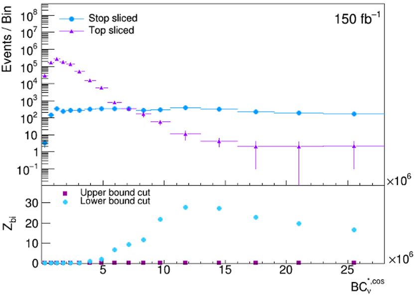
generators with non-trivial weight assignments (such as those that arise from jet matching
procedures). Instead, in a node-weighted network, the network can be populated with
events whose weights are defined in the normal manner. This is straightforward from the
perspective of network analysis, since network nodes are allowed to have any number of
attributes assigned to them, but it complicates the calculation of network metrics as we
shall see below. Although this analysis only considers weighted events from Monte Carlo
simulation, these methods are also applicable to searches with data-driven background
estimates that apply additional weights to appropriately selected data or Monte Carlo
events.
JHEP02(2021)160
2.2 Network metrics
Once a network has been defined, one can calculate a series of network metrics that char-
acterise the network topology. These include global metrics (defined for the network as a
whole), and local metrics (which we assume to be defined for each node of the network).
For a given selection of events, there is only one network that can be formed from all
of the selected events. It is possible in principle to infer the presence of new physics by
demonstrating that the global network metrics for the network of selected events depart
from a well-modelled Standard Model expectation. However, we will instead focus on local
metrics that will allow us to define attributes on an event-by-event basis. These can be
substituted for the kinematic variables that are used in a regular LHC event analysis, in
which searches for new physics are performed by placing selections on variables to define
regions of the data where the background is expected to be small.
The simplest example of a local network metric is the degree centrality of a node, which
is equal, for an unweighted network, to the number of other nodes that are connected to
it. In a social media network, for example, the degree centrality of a given person would
be equal to the number of their friends.
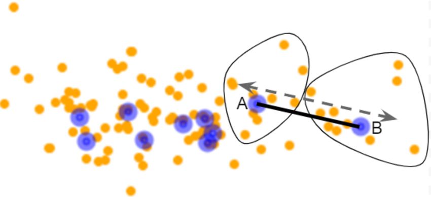
In a weighted network, the definitions of both local and global metrics must be updated
to take account of the fact that each node now represents a different number of effective
nodes. Node-weighted network measures can be defined based on the concept of node-
splitting invariance as detailed in ref. [22], and in the following we perform calculations
of node-splitting-invariant (n.s.i.) local network metrics using a custom version of the
pyunicorn package [23]. The full list of network measures that we utilise is as follows.
• The n.s.i. degree: for a given node ν, this is the weighted version of the degree
centrality, given by: P
i∈Nν+ wi
kν∗ = , (2.5)
(W + 1)
P
where W = i∈N wi is the sum of the weights of all nodes in the network. In our
analysis, W is equivalent to the total number of events expected at the LHC for our
assumed integrated luminosity.
• The n.s.i. average and maximum neighbours degree: the average neighbours degree
of a node ν represents the average size of the network region that an event linked to
–5–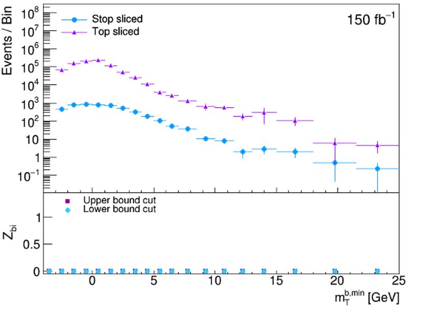
ν is linked to. The n.s.i. measure of this quantity is given by:
                                                         P             ∗
                                  ∗           1              i∈Nν+ wi ki
                                 knn,ν   =                               .                                (2.6)
                                           (W + 1)              kν∗

  One can also define an n.s.i. maximum neighbors degree, as
                                          ∗
                                         knnmax,ν = max ki∗ .                                             (2.7)
                                                         i∈Nν+

• The n.s.i. betweenness centrality: the shortest path betweenness centrality of a node

                                                                                                                  JHEP02(2021)160
  ν gives the proportion of shortest paths between pairs of randomly chosen nodes that
  pass through ν. If we label the random nodes by a and b, we have that:

                                 BCν = hnab (ν)/nab iab ∈ [0, 1],                                         (2.8)

  where nab is the total number of shortest paths from a to b, nab (ν) is the number of
  those paths that pass through ν, and we have defined the average of a function of
  node pairs by hh(i, j)iij = N12 i∈N j∈N h(i, j). One can write a formal expression
                                        P     P

  for this quantity by first noting that nab can be written as a sum over the tuples
  (t0 , . . . , tdab ), with t0 = a and tdab = b (dab is the number of links between the nodes
  a and b on the shortest path), where each tuple in the sum gives a contribution of 1
  if every node tl in the tuple is linked to its successor tl+1 , or 0 if at least one node
  is not linked to its successor. Both of these conditions are met if one simply takes
  the product of elements of the adjacency matrix for each pair of nodes in the tuple,
  allowing us to write

                                                 X                     dab
                                                                       Y
                        nab =                                                  atl−1 tl .                 (2.9)
                                 (to ,...,tdab )∈N dab +1 ,t0 =a,tdab =b l=1

  nab (ν) is given by a similar formula, except that, for some m in 1 . . . dab − 1, tm must
  equal ν:
                              ab −1
                             dX                        X                            dab
                                                                                    Y
                 nab (ν) =                                                                  atl−1 tl .   (2.10)
                             m=1 (to ,...,td )∈N dab +1 ,t0 =a,tm =ν,td =b l=1
                                            ab                         ab

  It is possible to make an n.s.i. version of this quantity based on a weighted average
  instead of an average (which would be consistent with the above formula in the limit
  that all node weights are 1), but the pyunicorn package instead uses a weighted sum,
  giving the n.s.i. betweenness centrality as:

                          BCν∗ = hn∗ab (ν)/n∗ab iwsum
                                                 ab   ∈ [0, W 2 /wν ],                                   (2.11)

  where we have defined the weighted sum of a function of pairs of nodes hh(i, j)iwsum
                                                                                   ij   =
  P     P
               w h(i, j)w   , and n ∗ (ν) and n∗ are defined below. The n.s.i. betweenness
    i∈N    j∈N i          j         ab         ab
  centrality values obtained for our examples below do not come close to saturating
  the maximum value of W 2 /wν .

                                               –6–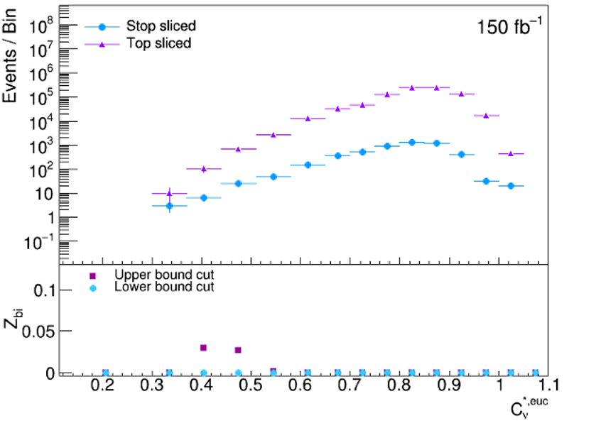
Formulae for n∗ab (ν) and n∗ab can be derived as follows. If a node s is hypothetically
split into two nodes s0 + s00 , any shortest path through s becomes a pair of shortest
paths (one of which passes through s0 , and the other of which passes through s00 ).
In addition, a shortest path from s00 to some b 6= s0 will never meet s0 . Thus, the
betweenness centrality can be made invariant under node splitting by making each
path’s contribution proportional to the product of the weights of the inner nodes,
but with the condition that we skip the weight wν in this product when calculating
nab (ν). Formally, we can write a modified n∗ab as:
ab −1
dX dab
n∗ab =
Y
JHEP02(2021)160
at0 t1 (wtl−1 atl−1 tl ), (2.12)
m=1 l=2
and a modified n∗ab (ν) as:
ab −1
dX dab
1
n∗ab (ν) =
X Y
at t (wtl−1 atl−1 tl ) . (2.13)
0 1
wν m=1 (to ,...,td
ab
)∈N dab +1 ,t 0 =a,tm =ν,tdab =b l=2
A geometric interpretation of the n.s.i. betweenness can be obtained by considering
the set of nodes of our node-weighted network {N } as a sample from a population
of points {N0 }. Each node ν in the network then represents some small cell Rν
of points in the geometric vicinity of ν in {N0 }. The n.s.i. betweenness can be
interpreted as an estimate of the probability density that a randomly-chosen shortest
path between two randomly-chosen points in the population network passes through a
specific randomly-chosen point in Rν . This is ultimately a measure of the importance
of the node ν in the network.
• The n.s.i. closeness centrality: another measure of node importance is the closeness
centrality, which is defined for a node ν by CCν = 1/ hdνi ii , where dνi is the number
of links on a shortest path from ν to i, or, if there is no path, ∞, and we have defined
the same average over nodes that was used previously. A larger value of CCν for a
node indicates a smaller average number of links to all other nodes in the network.
The n.s.i. version of this metric is given by:
W
CCν∗ = P ∗ ∈ [0, 1], (2.14)
i∈N wi dνi
where d∗νi is an n.s.i. distance function given by:
d∗νν = 1 and d∗νi = dνi for i 6= ν. (2.15)
The n.s.i. distance function is naively a little odd, and can be justified as follows. A
weighted version of CCν should give us the inverse average distance of ν from other
weight units or points rather than from other nodes. But for this to become n.s.i,
one has to interpret each node to have a unit (instead of zero) distance to itself since,
after an imagined split of a node s → s0 s00 , the two parts s0 and s00 of s have unit not
zero distance.
–7–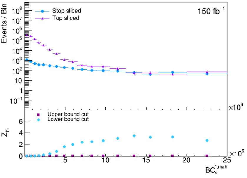
• The n.s.i. exponential closeness centrality: a limitation of the closeness centrality is
     that it receives very low values for nodes which are very close to most of the other
     nodes, but very far away from at least one of them. To prevent outlying nodes from
     skewing the closeness calculation for “typical”
                                                D      nodes, one can use the exponential
                                                       E
                                                   −d
     closeness centrality, defined as CCEC,ν = 2 νi . The n.s.i. measure is given by:
                                                                                 i
                                                             D         ∗
                                                                           Ew
                                           ∗
                                         CCEC,ν = 2−dνi                         ∈ [0, 1].                  (2.16)
                                                                            i

      where we have used the notation hg(ν)iw                          1    P
                                            ν =                        W        ν∈N       wν g(ν).

                                                                                                                    JHEP02(2021)160
   • The n.s.i. harmonic closeness centrality: the harmonic closeness centrality reverses
     the sum and reciprocal operations in the definition of closeness centrality, such that
     1/dνi contributes zero to the sum if there is no path from ν to i. The n.s.i. harmonic
     close centrality is given by:
                                           ∗
                                         CCHC,ν = h1/d∗νi iw
                                                           i ∈ [0, 1].                                     (2.17)

   • The n.s.i. local clustering coefficient: the local clustering co-efficient of a node ν is
     the probability that two nodes drawn at random from those linked to ν are linked
     with each other. It is given by:

                                                                            N 2 haνi aij ajν iij
                                      P          P
                                          i∈Nν       j∈Nν        aij
                             Cν =                                      =                               .   (2.18)
                                           kν (kν − 1)                           kν (kν − 1)

      The n.s.i. version is given by
                                     D              Ew
                                 W 2 a+   + +
                                      νi aij ajν               wν (2kν∗ − wν )

                                                        ij
                       Cν∗   =                               ∈                 , 1 ⊆ [0, 1].               (2.19)
                                         kν∗2                       kν∗2

   • The n.s.i. local Soffer clustering coefficient: an alternative form of the clustering
     coefficient proposed by Soffer and Vázquez [24] includes a correction that reduces the
     impact of degree correlations:

                                                 N 2 haνi aij ajν iij
                                 Cs,ν = P                                              ∈ [Cν , 1].         (2.20)
                                            i∈Nν (min(ki , kν )                 − 1)

      The n.s.i. version of this is given by:
                                                                 D                   Ew
                                                      W 2 a+   + +
                                                           νi aij ajν
                                  ∗                                                   ij
                                 Cs,ν =P                                                           .       (2.21)
                                                i∈Nν+   wi min(ki∗ , kν∗ )           ∈ [Cν∗ , 1]

For the case studies presented in this paper, networks of events are built for different
distance metrics after specified pre-selection criteria, which are detailed further in sections 4
and 5. For a given choice of distance metric, events are linked in the corresponding network
if their distance in the original space of kinematic variables is less than a chosen linking

                                                     –8–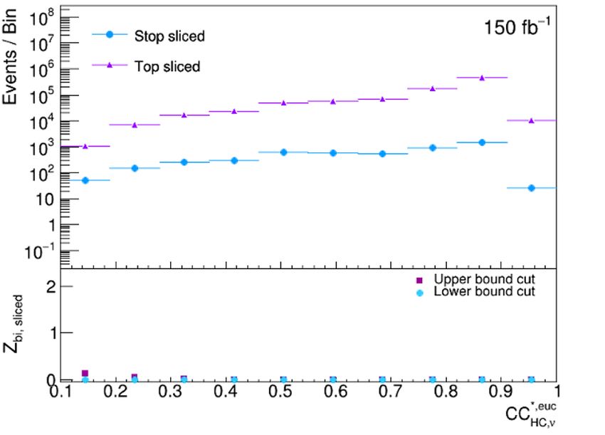
p                         ℓ                                      W±

                                             ℓ                              t
                                                              p                   b
                                     Z
                              χ̃02                                     t̃
                                                 χ̃01                           χ̃01

                                                 χ̃01                           χ̃01
                             χ̃±
                               1                                  t̃
                                     W                        p
                                             ν                              t          b

               p                         ℓ                                      W±

Figure 1. Feynman diagrams of the simplified supersymmetric models considered in (left) the

                                                                                                    JHEP02(2021)160
prototype electroweakino analysis and (right) the prototype stop pair analysis.

length l. The pre-selection criteria applied before the networks are constructed involve the
typical combinations of particle multiplicity selections and loose kinematic selections that
are encountered in SUSY searches at the LHC. Local network metrics are then used along
with further requirements on kinematic variables to define search regions analogous to
those used in existing LHC searches. Note that, unlike traditional analysis variables which
only depend on the kinematic properties of that event, the presence of a signal in the
LHC data would change the local network metrics for the background events in addition to
adding signal events to the various distributions. By comparing event yields obtained from
a background-only network (which mimics the data that would be expected in the absence
of a signal) to those from a signal-plus-background network (which mimics the data that
would be expected in the presence of a signal), estimates of the exclusion sensitivity are
calculated for the network driven analysis. These are compared to sensitivity estimates for
search regions defined only using conventional kinematic variables.
    The exclusion sensitivities are estimated using the RooStats framework [25], which pro-
vides a calculation for the binomial significance (Zbi ) associated with a number counting
experiment that tests between signal-plus-background and background-only hypotheses,
in the case that the background estimate has an uncertainty derived from an auxillary
measurement [26–28]. Our comparative results using this significance measure are encour-
aging and indicate that the network-based methods can offer significant improvements in
discovery potential. Since we do not have access to a full background analysis, complete
simulation of the detector systems, or the systematic uncertainties available to the experi-
mental collaborations, we do not show a full statistical analysis of the expected exclusion
and discovery reach, which is left for future studies.

3   Simulated signal and background event samples

To demonstrate our method we consider two case studies: supersymmetric electroweakino
and stop pair production, which will be discussed further in sections 4 and 5 respectively.
LHC searches are typically optimised on simplified models, and diagrams for the decays
considered in this paper are shown in figure 1.
    The electroweak neutralinos (χ̃0i=1,2,3,4 ) and charginos (χ̃±
                                                                 i=1,2 ) are the mass eigenstates
corresponding to linear combinations of the superpartners of the unbroken electroweak

                                                        –9–
gauge bosons and the supersymmetric Higgs particles. The mixing of the bino, wino, and
Higgsino states into the electroweakino states can greatly impact the resulting phenomenol-
ogy meaning that LHC searches are forced to make assumptions about the relative masses
and mixings of these states. In this paper, it is assumed that electroweakinos are produced
via wino-like χ̃± 0
1 − χ̃2 production, with subsequent decay to SM gauge bosons and the
lightest neutralinos, which are assumed to be pure bino states. We consider a model with
mχ̃± = mχ̃0 = 400 GeV, and mχ̃0 = 0 GeV. Both gauge bosons are assumed to decay
1 2 1
leptonically giving a 3-lepton final state, where the dominant background is SM diboson
(WZ) production. This model was not excluded in the three-lepton search channel in the
most recent 139 fb−1 analysis conducted by the ATLAS collaboration [29]. The results in
JHEP02(2021)160
this paper assume 150 fb−1 of integrated luminosity, which is comparable.
Our second example considers supersymmetric top quarks at the LHC, where it is
assumed that t̃1 t̃1 production dominates at the LHC, and the decay of the stop is presumed
to occur with 100% branching ratio to either a top quark and a lightest neutralino, χ̃01 ,
or a b quark and a lightest chargino. We consider a model with mt̃1 = 500 GeV, and
mχ̃0 = 280 GeV. This choice of benchmark SUSY model choice is motivated by the fact
1
that the model was not excluded by the most recent 36.1 fb−1 analysis conducted by the
ATLAS collaboration [30], and it can be expected to be challenging to observe due to the
fact that the kinematic properties of the top quarks produced are rather similar to those
expected in the Standard Model. We will develop a prototype analysis in the 1 lepton final
state, in which one of the top quarks is assumed to decay hadronically, whilst the other
decays leptonically, which is typically the most constraining final state. The dominant
SM background in this final state is top quark production (including both top pair and
single top production). In a real analysis, there would be a small contribution from events
containing a W boson produced in association with jets, but we neglect this for our proof of
principle. We note that, in the final stages of our work, the ATLAS collaboration released
a zero lepton stop pair production search utilising 139 fb−1 of data which does exclude this
benchmark model [31].
For both case studies, the signal and dominant SM background (diboson WZ for the
electroweakino case and top quark production for the stop case) are simulated with Pythia
8.240 [32] using the CTEQ6L1 PDF set [33], and an LHC detector simulation is performed
using Delphes 3.4.1 [34–36], using the default ATLAS detector card. Jets are recon-
structed using the anti-kT algorithm with a radius parameter R=0.4 [37] using the FastJet
package [38]. In normalising the electroweakino signal to the relevant integrated lumi-
nosity, we use the next-to-leading-order plus next-to-leading-log cross-section provided in
refs. [39, 40], whilst cross-section used for normalisation of the stop sample is the next-
to-next-to-leading-order plus approximate next-to-next-to-leading log cross-section derived
from refs. [41–44]. For the SM backgrounds, the WZ sample uses the next-to-next-to-
leading order cross-section presented in ref. [45] and the top sample uses the next-to-next-
to-leading-order plus next-to-next-to-leading log tt̄ cross-section derived from refs. [46–52].1
1
Note that this gives us an approximate weighting of the top background, since the subdominant single
top contribution will be scaled by the same cross-section as the tt̄ contribution.
– 10 –To ensure that the extreme tails of kinematic distributions are adequately sampled,
both case studies use “sliced” background event samples, and the stop cases uses “sliced”
signal event samples. For the stop case study samples are generated in slices of HT , whilst
the electroweakino samples are sliced in p̂T , the transverse momenta in the rest frame of
the hard scattering process. For the electroweakino case all of the events passing the pre-
selection defined in section 4 were used to build the network, however for the stop case to
speed up the network calculations for our proof of principle, we take a subsample of 10,000
events for both the signal and background, and adjust their weights accordingly. We also
make use of inclusive MC samples (i.e. with no slicing) for testing, and for plotting the
distance metrics, since the inclusive samples adequately describe the distributions of the
JHEP02(2021)160
distance metrics that one expects to see in LHC data, in the regions of interest.
We have performed a variety of checks that the network metrics we use are indeed safe
under the reweighting of events, using both the inclusive samples, and the sliced events.
These checks are presented for both of the electroweakino and stop examples in appendix A.
This study also considers the assumptions associated with using n.s.i. network metrics on
theoretical grounds, i.e. that a weighted node can be taken to represent a group of identical
nodes which possess full internal connectivity and identical external connectivity. In the
subsequent sections we only present quantitative results for n.s.i. metrics that we argue are
robust under these conditions; the n.s.i. degree and n.s.i. closeness, harmonic closeness and
exponential closeness centralities. The betweenness centrality may not be robust under the
external connectivity assumption and could thus be affected by node-weight-dependent
biases. For this reason we only show qualitative results that demonstrate its potential.
Improvements to methods for constructing node-weighted networks that could improve the
accuracy of the second assumption are an interesting avenue for future study.
4 Case study 1: the search for electroweakinos
4.1 Electroweakino analysis design
As our first example of the application of network analysis techniques to an LHC search,
we will consider the hunt for supersymmetric electroweakinos at the LHC. The first step
in our analysis is to apply a pre-selection consistent with a 3 lepton electroweakino search.
We require there to be exactly three light leptons (electrons or muons), with transverse
momentum pT > 25 GeV and pseudorapidity |η| < 2.5. We do not apply additional pseudo-
rapidity or isolation requirements to the default electron/muon reconstruction provided by
Delphes3 [34–36]. The default settings restrict electrons, photons and muons to |η| < 2.5,
while jets and missing transverse energy are restricted to |η| < 4.9. We further require there
to be no b-tagged jets and at most 1 non-b-tagged jet in the event with pT > 25 GeV and
|η| < 2.4, and for the dilepton invariant mass of an opposite-sign same-flavour pair in the
event to satisfy |mll − mZ | < 10 GeV. When investigating the potential improvements in
sensitivity from including network metrics in the definition of search regions, we consider a
series of variables that are typically used to discriminate electroweakino events from diboson
events, choosing to focus on those whose distributions over all events show the greatest
difference between our benchmark signal point and the diboson background. These are:
– 11 –• The missing transverse energy ET miss , which represents the momentum imbalance
transverse to the beam direction and can be used to infer the presence of weakly
interacting neutral particles escaping the detector.
• ml,min
T
miss ), m (l , E miss ), m (l , E miss ))
: defined as min(mT (l1 , ET T 2 T T 3 T
• pT (Z): the reconstructed transverse momentum of the Z boson.
+ −
• ∆Φ(lZ , lZ ): the azimuthal angle between the two leptons associated with the Z boson,
which are taken to be the same-flavour opposite sign pair whose di-lepton invariant
mass is closest to the Z-boson mass in the case of any ambiguity (with the remaining
JHEP02(2021)160
lepton assigned to the W -boson).
• ∆Φ(Z, lW ): the azimuthal angle between the reconstructed Z boson and the lepton
coming from the W boson.
When constructing the network for a given event sample these variables are scaled to
equalise their weight in the analysis and account for their differing units. This “median”
scaling is performed by subtracting the median of the variable’s distribution in the back-
ground sample and normalising by the median absolute deviation (MAD). The MAD is
calculated by subtracting the median of the background dataset from each point to produce
a new dataset, then finding the median of the new dataset. A median scaling is chosen
rather than a mean scaling to avoid being overly sensitive to tail effects. The distance
metrics defined in section 2 are then calculated for a dataset containing 4000 of our simu-
lated signal events and 4000 of our simulated SM events. Distributions of these distances,
normalised to unit area, are shown for signal and background events in figure 2, where
we have separated the distributions for signal-signal, signal-background and background-
background distances.
Focussing on the signal-signal and background-background distributions, we see that
these metrics exhibit reasonably large differences between the signal and background pro-
cesses, indicating the presence of different typical scales at which events are expected to be
clustered in the two cases. It is interesting to note that, in some cases, the signal-signal and
background-background roles are reversed; the Bray-Curtis, correlation and cosine metrics
all have the signal-signal distributions being more concentrated at small distances than
the background-background distributions. This raises the option of flipping the friendship
condition to occur if the distance in kinematic space is greater than the linking length,
although we continue to adopt the standard definition in the following analysis for consis-
tency between distance metrics. For each distance metric dij between pairs of events i and
j, we define the adjacency matrix for the graph network by using the definition in Equa-
tion 2.4. The linking length l is chosen to be indicative of a characteristic scale of separation
of background events, which differs from that of signal events. This then ensures that back-
ground events are well-connected in the networks, whilst signal events typically have fewer
connections. Our final choices for each distance metric are summarised in table 1.
After applying the event pre-selection, and with our definitions of “friendship” in place,
we build networks for each distance metric and calculate, for each event, the local metrics
– 12 –0.22 0.18
Normalised Entries
Normalised Entries
0.2 dbray bkg-bkg 0.16 dcheb bkg-bkg
dbray bkg-sig dcheb bkg-sig
0.18
dbray sig-sig 0.14 dcheb sig-sig
0.16
0.12
0.14
0.12 0.1
0.1 0.08
0.08
0.06
0.06
0.04
0.04
0.02 0.02
0 0
0 0.5 1 1.5 2 2.5 3 3.5 4 4.5 5 0 5 10 15 20 25 30
JHEP02(2021)160
dbray dcheb
(a) Bray-Curtis (b) Chebyshev
0.08
Normalised Entries
Normalised Entries
dcity bkg-bkg 0.3 dcorr bkg-bkg
0.07 dcity bkg-sig dcorr bkg-sig
dcity sig-sig 0.25 dcorr sig-sig
0.06
0.05 0.2
0.04
0.15
0.03
0.1
0.02
0.05
0.01
0 0
0 10 20 30 40 50 60 0 0.2 0.4 0.6 0.8 1 1.2 1.4 1.6 1.8 2
dcity dcorr
(c) Cityblock (d) Correlation
0.03
Normalised Entries
Normalised Entries
0.3 dcos bkg-bkg deuc bkg-bkg
dcos bkg-sig 0.025 deuc bkg-sig
0.25 dcos sig-sig deuc sig-sig
0.02
0.2
0.015
0.15
0.1 0.01
0.05 0.005
0 0
0 0.2 0.4 0.6 0.8 1 1.2 1.4 1.6 1.8 2 0 5 10 15 20 25 30
dcos deuc
(e) Cosine (f) Euclidean
0.05
Normalised Entries
0.045 dmah bkg-bkg
dmah bkg-sig
0.04 dmah sig-sig
0.035
0.03
0.025
0.02
0.015
0.01
0.005
0
0 2 4 6 8 10 12 14 16 18 20
dmah
(g) Mahalanobis
Figure 2. Distributions of the distance metrics used in our prototype electroweakino search.
– 13 –Distance metric Linking length
dbray 0.7
dcheb 4.8
dcity 12
dcorr 0.6
dcos 0.6
deuc 6.4
dmah 4.8
Table 1. Linking length values used for each distance metric for our prototype electroweakino
JHEP02(2021)160
analysis.
defined in section 2. Our analysis will proceed in two stages, designed to reflect how it
could be performed in practice at the LHC:
• In this section, we use a signal-plus-background network to design signal regions that
would be sensitive to our chosen electroweakino benchmark point, using a knowledge
of which events in our simulated network are background events, and which are signal
events. Within the ATLAS and CMS collaborations, this would correspond to using
MC samples to design and optimise signal regions, using only one set of generated
background events. Hypothetical significance results are obtained by placing selec-
tions on the original variables, and local network metrics, and counting the number of
signal and background events in the resulting search region. For this procedure to be
valid, it is essential that the background contribution to the signal-plus-background
network metric distributions does not change significantly from the background dis-
tribution that would result from only having the background present in the network.
We have checked this explicitly for all variables that are used to define our optimum
analyses below.2
• In section 4.2, we develop a realistic example of an LHC exclusion test by simulating
an independent set of background events that corresponds to the LHC data that
would be obtained in the absence of a signal. These MC events are to be interpreted
as “mock LHC data”, and we build background-only networks from those events
to represent the networks that would be obtained in such an LHC dataset. The
yields in our search regions for the mock LHC data can then be compared to the
yields expected from our signal-plus-background network analysis to determine the
exclusion significance of our benchmark model (which now incorporates the effect of
statistical fluctuations in the real LHC data). In practise, this test could be repeated
on a variety of signal models, to generate exclusion limits in, for example, simplified
model parameter planes.
2
As an alternative, one could split the background MC into two sets, and optimise the variable selections
using both a signal-plus-background network, and a background-only network. We do not pursue that option
in this paper, in order to reduce our simulation time.
– 14 –The metric calculations are computationally expensive to evaluate. For the electroweakino
example, we used all events that pass the pre-selection (which amounts to just over 10,000
signal and 10,000 background events before weighting). We are confident that one could
evaluate network metrics for O(100, 000) network events with a suitable parallellisation
of the network metric calculations, making the use of network variables after a looser
pre-selection a realistic possibility within the ATLAS and CMS collaborations. With our
chosen distance metrics, we have 7 × 8 =56 new variables in total, and we are also free to
retain the original variables for extra kinematic selections.
After building the networks, we explored a variety of potential event selections that
used either the network metrics alone, the original kinematic variables alone, or a combi-
JHEP02(2021)160
nation of the original kinematic variables and network metrics. Including tighter kinematic
requirements in the pre-selection before building the graph network weakened the sensitiv-
ity of the network-driven searches, due to the increased kinematic similarity of the signal
and background events that pass tighter kinematic selections. The five kinematic variables
are shown in figure 3. The lower panel of each figure shows the binomial significance Zbi
for either an upper cut or lower cut on the variable at the value given on the horizontal
axis, assuming a total systematic uncertainty of 15% (chosen to be consistent with numbers
quoted by the ATLAS run-2 searches in the 3-lepton channel [29, 53]). This significance
calculation also includes the statistical uncertainty of the background which is added to
the systematic uncertainty in quadrature. When the signal or background weighted event
yield drops below 3 events, the Zbi is set to 0. Differences in shape between the signal and
SM distributions are clearly apparent, but no selection on a single kinematic variable is
able to achieve an expected exclusion sensitivity at 95% confidence level (corresponding to
Zbi = 1.64) for our chosen benchmark point.
These distributions can be contrasted with the distributions for the network metrics
in the signal-plus-background network. In figures 4–5, we show various useful network
metrics for the Euclidean, Chebyshev, cityblock, Bray-Curtis and cosine distance metrics.
The supersymmetric events consistently show lower values of kν∗ as well as the clustering and
closeness variables. This suggests that the supersymmetric events form fewer connections
with other events than the Standard Model events, and that the events they do connect
with are also sparsely connected. This arises from a combination of factors including the
different typical lepton four-momenta expected in the SUSY case (given that the final state
has a higher multiplicity), different signal distributions for variables which have well-defined
kinematic endpoints for the background, and the fact that the smaller number of SUSY
events limits the number of possible connections relative to background events. The rare
and complex nature of the SUSY events for our benchmark model can be expected to be
common among many BSM model processes, suggesting that these network metrics could
also be useful for other cases. This includes the more complex supersymmetry models
favoured by recent global fits that significantly depart from simplified model assumptions.
Taken as a set, the local network metric distributions offer a large set of variables that
offer greater discrimination between signal and background than can be obtained with the
original kinematic variables.
To find optimum kinematic selections for potential analyses, we first consider each
network metric in turn. We determine which variables will give the highest significance
– 15 –Events / Bin
Events / Bin
Electroweak SUSY signal 150 fb−1 Electroweak SUSY signal 150 fb−1
104 WZ 104 WZ
3 3
10 10
10 2
102
10 10
1 1
10−1
10− 1
Upper bound cut Upper bound cut
1 Lower bound cut 0.6 Lower bound cut
Zbi
0.4
Zbi
JHEP02(2021)160
0.5
0.2
0 0
0 10 20 30 40 50 0 5 10 15 20 25 30 35
E miss
T
m l,min
T
miss
(a) ET (b) ml,min
T
Events / Bin
Events / Bin
104 Electroweak SUSY signal 150 fb−1 104 Electroweak SUSY signal 150 fb−1
WZ WZ
3 3
10 10
2
10 102
10 10
1 1
10− 1 10− 1
Upper bound cut 0.15 Upper bound cut
0.3 Lower bound cut Lower bound cut
0.2 0.1
Zbi
Zbi
0.1 0.05
0 0
−3 −2 −1 0 1 −5 −4 −3 −2 −1 0 1
+ -
∆Φ(l , lZ) ∆Φ(Z,l )
Z W
+ −
(c) ∆Φ(lZ , lZ ) (d) ∆Φ(Z, lW )
Events / Bin
Electroweak SUSY signal 150 fb−1
104 WZ
3
10
102
10
1
−1
10
1.5 Upper bound cut
Lower bound cut
1
Zbi
0.5
0
0 10 20 30 40 50
p (Z)
T
(e) pT (Z)
Figure 3. Event rates as a function of the kinematic variables used in our prototype electroweakino
search, with the median scaling applied. Events in the overflow bin are not shown in the distribution
but are included in the Zbi calculation.
– 16 –Events / Bin
Events / Bin
Electroweak SUSY signal 150 fb−1 104 Electroweak SUSY signal 150 fb−1
104 WZ WZ
3
10
3 10
10 2 102
10 10
1 1
10− 1 10− 1
Upper bound cut Upper bound cut
Lower bound cut Lower bound cut
1 1
Zbi
Zbi
0.5 0.5
0 0
0 0.1 0.2 0.3 0.4 0.5 0.6 0.7 0.8 0.9 1 0 0.1 0.2 0.3 0.4 0.5 0.6 0.7 0.8 0.9 1
*,euc *,city
kν kν
JHEP02(2021)160
(a) kν∗,euc (b) kν∗,city
Figure 4. Event rates as a function of useful network metrics for our prototype electroweakino
analysis calculated using dcity . Events in the overflow bin are not shown in the distribution but are
included in the Zbi calculation.
Requirement Nsignal Nbackground Zbi
∗,corr
kν∗,euc < 0.003, CCEC,ν > 0.324 7.78 ± 0.17 6.53 ± 1.29 1.96
∗,euc ∗,corr
kν < 0.003, CCHC,ν > 0.656 8.45 ± 0.18 7.52 ± 1.45 1.96
∗,city
kν < 0.004, kν∗,cos > 0.343 5.86 ± 0.15 3.20 ± 1.05 1.89
∗,cos
kν∗,city < 0.004, CCHC,ν > 0.646 7.43 ± 0.16 5.67 ± 1.42 1.89
∗,city ∗,corr
kν < 0.004, kν > 0.359 7.34 ± 0.16 5.43 ± 1.10 2.04
∗,city ∗,corr
kν < 0.004, CCEC,ν > 0.323 8.13 ± 0.17 7.15 ± 1.44 1.93
∗,city ∗,corr
kν < 0.004, CCHC,ν > 0.656 8.17 ± 0.17 7.27 ± 1.45 1.92
Table 2. Examples of binomial significances for search regions that provide exclusion sensitivity
without reducing yields below 3 events. The errors only include the statistical error.
based on a single upper or lower cut, considering many possible cut values for each variable.
This is then iteratively repeated with the additional variables until the number of signal
and background events passing the combined selections drops below 3 in each case. Some
examples of the Zbi values and event yields obtained for promising search regions which
provide Zbi > 1.64 are shown in table 2. This calculation includes both the statistical
uncertainty on the event yields, and an assumed systematic uncertainty of 15%.
4.2 Results of realistic electroweakino exclusion test
Having defined signal regions using hypothetical signal-plus-background networks, we now
compare the yields derived from the signal-plus-background networks with the background-
only networks derived from our mock LHC dataset. This determines the exclusion sensi-
tivity for our benchmark point that one would obtain with actual LHC data. The binomial
significance is once again calculated with an error on the background yield that includes
the statistical uncertainty plus an additional 15% systematic uncertainty. table 3 com-
pares the expected sensitivity of these regions with that obtained in some representative
– 17 –Events / Bin
Events / Bin
104 Electroweak SUSY signal 150 fb−1 104 Electroweak SUSY signal 150 fb−1
WZ WZ
3 3
10 10
10 2
102
10 10
1 1
10− 1 10− 1
Upper bound cut Upper bound cut
0.15 Lower bound cut 0.15 Lower bound cut
0.1 0.1
Zbi
Zbi
JHEP02(2021)160
0.05 0.05
0 0
0.1 0.15 0.2 0.25 0.3 0.35 0.4 0.52 0.54 0.56 0.58 0.6 0.62 0.64 0.66 0.68 0.7 0.72
*,corr *,corr
kν CCHC,ν
∗,corr
(a) kν∗,corr (b) CCHC,ν
Events / Bin
Events / Bin
104 Electroweak SUSY signal 150 fb−1 104
Electroweak SUSY signal 150 fb−1
WZ WZ
3
10 10
3
2
10 102
10 10
1 1
10− 1 10−1
Upper bound cut Upper bound cut
0.15 Lower bound cut 0.15 Lower bound cut
0.1 0.1
Zbi
Zbi
0.05 0.05
0 0
0.28 0.29 0.3 0.31 0.32 0.33 0.34 0.35 0.1 0.15 0.2 0.25 0.3 0.35 0.4
*,corr *,cos
CCEC,ν kν
∗,corr
(c) CCEC,ν (d) kν∗,cos
Events / Bin
Electroweak SUSY signal 150 fb−1
104 WZ
3
10
102
10
1
−1
10
Upper bound cut
0.15 Lower bound cut
0.1
Zbi
0.05
0
0.52 0.54 0.56 0.58 0.6 0.62 0.64 0.66 0.68
*,cos
CCHC,ν
∗,cos
(e) CCHC,ν
Figure 5. Event rates as a function of useful network metrics for our prototype electroweakino
analysis calculated using dcorr and dcos . Events in the overflow bin are not shown in the distribution
but are included in the Zbi calculation.
– 18 –Normalised Events / Bin
Normalised Events / Bin
104 S+B 150 fb−1 104 S+B 150 fb−1
B B
3 3
10 10
2
10 102
10 10
1 1
−1 −1
10 10
2 2
S+B / B
S+B / B
1 1
0.52 0.54 0.56 0.58 0.6 0.62 0.64 0.66 0.68 0.7 0.72 0 0.1 0.2 0.3 0.4 0.5 0.6 0.7 0.8 0.9 1
*,corr *,city
CCHC,ν
JHEP02(2021)160
kν
∗,corr
(a) CCHC,ν (b) kν∗,city
∗,euc
Figure 6. Event rates as functions of Cs,ν and kν∗,city for W Z background events calculated from
either the signal-plus-backround or background-only network. These two networks use different sets
of simulated W Z events. Events in the overflow bin are not shown in the distribution.
search regions constructed using only conventional kinematic variables. These selections
are loosely inspired by the regions in the ATLAS 36.1fb−1 search [30], but generally have
tighter requirements on ET miss and M l,min . We also impose slightly different pre-selection
T
requirements (we require njets < 2 whereas the ATLAS search region was inclusive in light
jet multiplicity, but had “binned” regions considering the 0 and >0 light jet categories
separately). The Zbi values differ from those of the previous section as expected, primarily
due to statistical fluctuations in the assumed LHC dataset. As is demonstrated in fig-
ure 6, which superimposes example background distributions taken from the background
component of the signal-plus-background networks and the background-only networks, the
general shape of the distributions are the same. This validates our previous procedure of
designing search regions using signal-plus-background networks alone, and ultimately tells
us that, for the chosen variables, the addition of rare signal events to the network does not
subtantially alter the connection properties of background events. It remains the case that
network methods provide exclusion sensitivity for the benchmark SUSY model, and they
also outperform the analysis that uses cuts on the original kinematic variables.
5 Case study 2: the search for stop quarks
5.1 Stop analysis design
As a second demonstration of the application of network analysis to an LHC search, we
consider the search for supersymmetric top quarks at the LHC. This is to determine if
the apparent gains seen in the previous section are generic to all final states and signal
topologies, or whether the same network metrics that work well in the electroweakino case
fail in another example.
Before building the network we require there to be exactly one electron or muon, with
transverse momentum pT > 25 GeV, at least 2 b-jets (with pT > 30 GeV), and a missing
transverse energy, ET miss , greater than 100 GeV. We have then examined a number of
– 19 –Requirement(s) Nb−only Ns+b Zbi
∗,corr
kν∗,euc < 0.003, CCEC,ν > 0.324 7.27 ± 1.17 14.31 ± 1.3 1.76
∗,euc ∗,corr
kν < 0.003, CCHC,ν > 0.656 8.43 ± 1.36 15.97 ± 1.46 1.73
∗,city
kν < 0.004, kν∗,cos > 0.343 3.48 ± 0.85 9.06 ± 1.06 1.90
∗,cos
kν∗,city < 0.004, CCHC,ν > 0.646 6.21 ± 1.29 13.1 ± 1.42 1.77
∗,city ∗,corr
kν < 0.004, kν > 0.359 6.08 ± 1.13 12.77 ± 1.11 1.79
∗,city ∗,corr
kν < 0.004, CCEC,ν > 0.323 7.77 ± 1.46 15.29 ± 1.45 1.74
∗,city ∗,corr
kν < 0.004, CCHC,ν > 0.656 7.17 ± 1.31 15.45 ± 1.46 2.01
∗,city ∗,corr
knn,ν < 0.009, CCHC,ν > 0.659 4.4 ± 0.87 9.5 ± 0.85 1.63
JHEP02(2021)160
pT (Z) > 160 GeV, ET miss
> 100 GeV, ml,min
T > 150 GeV 93.93 ± 7.66 105.28 ± 7.55 0.47
miss
pT (Z) > 160 GeV, ET > 200 GeV, ml,min
T > 150 GeV 28.55 ± 3.83 34.99 ± 3.62 0.64
pT (Z) > 160 GeV, ET miss
> 300 GeV, ml,min
T > 150 GeV 7.05 ± 1.59 13.41 ± 1.78 1.48
Table 3. Yields in our electroweakino search regions for our mock LHC data set (Nb−only ) and
our mock MC set (Ns+b ). Also shown is the sensitivity of search regions using only the original
kinematic variables. The errors quoted are statistical only, whilst the Zbi calculation uses a relative
background uncertainty.
variables that are normally used in stop searches, choosing the following set that show good
discrimination between the background and signal processes for our benchmark signal point:
• The leading jet transverse momentum pjT1 ;
miss ;
• the value of the missing transverse momentum ET
• the minimum value of the transverse mass, mb,min
T formed
q
by the two b-jets and
missing transverse energy in the event. mbT is defined as 2pbT ET miss [1 − cos(∆φ)],
with pbT signifying the tranverse momentum of each b-jet, and ∆φ giving the difference
in φ between the each b-jet and the missing transverse momentum;
• the minimum value of the invariant mass formed by the lepton and each of the two
b-jets in the event, mmin
bl . For the top pair production process, this has a maximum
value, whilst signal events can have higher values;
• the scalar sum of the moduli of the transverse momenta for the lepton and the 2
b-jets, which we refer to as HT ;
• the asymmetric mT 2 value, amT2 defined in refs. [54–58].
We show histograms of event rates as functions of these variables after the pre-selection
in figure 7, with the samples scaled using the “background median” procedure defined
previously. In all cases the signal lies substantially below the background across the entire
range of the distribution. The variables are used in the calculation of our various distance
metrics, exactly as we did in the previous section. Similar histograms of the distance
metrics are provided for our stop example in figure 8. Based on these plots, we select the
– 20 –Distance metric Linking length
dcorr 0.7
dcos 0.8
deuc 5.5
dmah 4.0
Table 4. Linking length values used for each distance metric for our prototype stop analysis.
linking lengths given in table 4, where we note that we have suppressed metrics that did not
turn out to be useful for any local network metric. As in the electroweakino example, the
JHEP02(2021)160
correlation and cosine metrics have the signal being more concentrated at small distances
than the background. We again retain the standard friendship condition when building
our networks, where two nodes are linked by an edge if they are closer in distance than the
linking length.
In figure 9, we show the network metrics that were used in the previous example,
and that are considered robust under the theoretical reasoning described in appendix A.
Although the distributions show modest differences in shape in some cases, there is not
enough separation of the signal and background distributions to render these particular
local network metrics useful in stop searches. We found no combination of selections on
these variables plus the original kinematic variables that gave sensitivity for exclusion at
the LHC. It remains possible that different choices of the original kinematic variables used
to build the network might change this picture, but it is clear that the use of local network
metrics does not automatically give sensitivity to BSM physics signals.
Before concluding this section, it is worth noting that some network metric distribu-
tions show much greater signal-background separation (see figure 10). For example, the
betweenness measures typically fall off much faster for top events than for stop events. This
is particularly true for networks built using the correlation and cosine distance metrics, for
which the betweenness centrality distributions for the background do not show evidence of
a flatter tail which is apparent in the case of the Mahalanobis betweenness. More modest
discrimination comes from the Euclidean local clustering, the Euclidean local soffer clus-
tering and the cosine average neighbors degree. Although we currently recommend caution
on the use of these metrics (due to the potential violation of the n.s.i. external connectivity
assumption detailed in appendix A), we feel that further investigation of the robustness of
these metrics in LHC use cases is a strong avenue for future work.
6 Discussion
For our electroweakino example, we have shown that the network variables provide exclu-
sion potential for a benchmark point that has just been excluded by a three lepton ATLAS
search performed using 139 fb−1 of data recorded by the ATLAS experiment.
So far, we have compared the efficacy of the network variables with the original kine-
matic variables by comparing prototype cut-and-count analyses, and by discussing the
shape of the various variables. In order to more comprehensively compare the effective-
– 21 –You can also read