Reservoir computing based on a silicon microring and time multiplexing for binary and analog operations
←
→
Page content transcription
If your browser does not render page correctly, please read the page content below
www.nature.com/scientificreports
OPEN Reservoir computing based
on a silicon microring and time
multiplexing for binary and analog
operations
Massimo Borghi*, Stefano Biasi & Lorenzo Pavesi
Photonic implementations of reservoir computing (RC) promise to reach ultra-high bandwidth of
operation with moderate training efforts. Several optoelectronic demonstrations reported state
of the art performances for hard tasks as speech recognition, object classification and time series
prediction. Scaling these systems in space and time faces challenges in control complexity, size and
power demand, which can be relieved by integrated optical solutions. Silicon photonics can be the
disruptive technology to achieve this goal. However, the experimental demonstrations have been
so far focused on spatially distributed reservoirs, where the massive use of splitters/combiners and
the interconnection loss limits the number of nodes. Here, we propose and validate an all optical RC
scheme based on a silicon microring (MR) and time multiplexing. The input layer is encoded in the
intensity of a pump beam, which is nonlinearly transferred to the free carrier concentration in the
MR and imprinted on a secondary probe. We harness the free carrier dynamics to create a chain-like
reservoir topology with 50 virtual nodes. We give proof of concept demonstrations of RC by solving
two nontrivial tasks: the delayed XOR and the classification of Iris flowers. This forms the basic
building block from which larger hybrid spatio-temporal reservoirs with thousands of nodes can be
realized with a limited set of resources.
The last decade has seen a flourish of new machine learning (ML) methods and applications, sometimes sur-
passing the human’s capabilities in solving hard tasks such as object recognition1,2, playing board games3 or
lipreading4. Among the different approaches, Reservoir Computing (RC) has attracted growing interests due
to its trade-off between performance and training complexity5. RC is a machine learning paradigm inspired by
Recurrent Neural Networks (RNN) where a set of input stimuli triggers the nonlinear dynamics of a network of
thousands of nodes, typically sparsely connected by fixed random weights6. The reservoir processes the infor-
mation and maps the original input space into one of increased dimension, thus mimicking the sequence of
nonlinear transformations of feed forward neural networks. In contrast with these, only the nodes in the readout
layer are trained, while the network separability is guaranteed by the highly nonlinear dynamics of the reservoir.
The training process is thus reduced to a linear combination of the output states of the reservoir, which can be
implemented with minimal computational resources. At the heart of RC lies the fact that loose conditions on
the topology of the reservoir are required for operation7, which find realization in a variety of physical systems.
Among these, photonic RC promises to be the ideal platform for hardware acceleration, due to an ultra-high
bandwidth of operation and ease of i mplementation8–11. Excellent demonstrations exist, which fall into two dis-
tinct categories: spatial and delayed-node reservoirs. The first has a close analogy with RNN, in which nodes are
spatially distributed and can be physically interconnected, as in the network of Semiconductor Optical Ampli-
fiers proposed i n12, or can be software-connected, as the pixels of the spatial light modulator i n13. Delayed node
reservoirs use instead a single physical node for computation. Here, the nodes are virtual and multiplexed in
time along an optical delay loop10. The network connectivity is given by the inertia of the system9, or by asyn-
chronously sampling the readout nodes with respect to the time of injection of the i nputs8,14. Implementations
often use optoelectronic delay loops embedding nonlinear elements as Mach Zehnders or phase modulators9,
DFB lasers15, VCSELs16 or p hotodetectors8. Being built from off-the shelf optics and electronics, these systems
operate at GHz speed and possess thousands of nodes. State of the art performances have been demonstrated
on several benchmarking tests, as chaotic time series prediction, nonlinear channel equalization and speech
Nanoscience Laboratory, Department of Physics, University of Trento, Via Sommarive 14, 38123 Trento, Italy.
*
email: massimo.borghi@unitn.it
Scientific Reports | (2021) 11:15642 | https://doi.org/10.1038/s41598-021-94952-5 1
Vol.:(0123456789)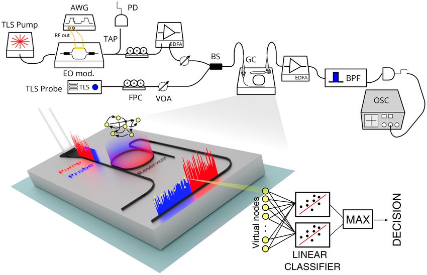
www.nature.com/scientificreports/
recognition. However, to satisfy the growing demand of more challenging tasks, the number of virtual nodes
and their interconnection complexity is foreseen to increase over the next years. Scaling these parameters with
bulk optoelectronic solutions will soon become unpractical for both spatial and delay-loop architectures. This
is why numerous schemes based on integrated optics have been proposed, and some of them experimentally
demonstrated. Silicon photonics is the ideal platform for very large scale integration, offering the possibility to
fabricate hundreds of individually addressable and reconfigurable optical elements in few cm217. While coherent
feed-forward neural networks have been recently reported18,19, the number of experimental demonstrations of
RC based on silicon photonics still remain very limited15,20,21. Most of the proposed schemes focus on passive
spatially distributed reservoirs made by small matrices of waveguides20,22, photonic crystal cavities23 or ring
resonators24–26. The fading memory of these systems is given by the delay lines which connect the nodes, or by
the photon lifetime of the cavities. This memory spans from few ps to some ns. The nonlinearity is typically
provided by the use of square law photodetectors, except for the theoretical w orks24–26, where it is given by the
nonlinear response of a MR. The scale of the reservoir is limited by the loss of the delay lines and by the repeated
use of splitters (coherent combining) which create the connectivity of the n etwork27. The integration of single
nodes with delayed feedback eliminates the interconnection problem, but also faces challenges, since lossy delay
loops of the order of few ns are required to store hundreds of virtual nodes with ps s eparation15,21. It is natural to
seek the use of hybrid spatio-temporal architectures as an optimal trade-off solution. These may adopt a small
scale spatial topology with sparse connectivity, where each physical node can accommodate few hundreds of
time multiplexed virtual nodes, similar to what is suggested in28 and recently demonstrated on a silica c hip29.
It is worth noting that there are other approaches to increase the dimensionality of the network. Indeed, the
exploitation of other degrees of freedom have been proposed, such as polarization and the longitudinal modes
of a Fabry Perot cavity16,30.
In this work, we propose and experimentally validate a silicon MR and time multiplexing as a single physical
node. The input space is encoded in time bins of different light intensity, which are injected in the device. The
time bin duration is of the same order of the response of the nonlinear node, which triggers a transient state in
the free carrier population. The carrier dynamics defines the connections between the virtual nodes. Specifically,
in contrast to the systems shown in ref.24–26, we adopt a scheme in which the input information is nonlinearly
transferred from a pump to a weak continuos wave (CW) probe laser inside the MR. This is achieved by gen-
erating carriers through Two Photon Absorption (TPA) and then by imprinting their signature on the probe
intensity by Free Carrier Dispersion (FCD), which shifts the resonance frequency of the cavity. The system does
not require active materials and does not rely on photodetection to induce nonlinearities, being these naturally
provided by TPA. The strength of information transfer is two orders of magnitude higher than the one mediated
by Kerr, and occurs at modest input power thanks to the light enhancement inside the MR (see supplementary
material). The reservoir operates at the rather slow timescale of 45 ns (∼ 20 MHz ), which is due to the unusu-
ally long carrier lifetime in our device. However, silicon waveguides with sub-ns carrier lifetimes are standard
components of large scale photonic circuits31,32, and the use of carrier depletion modulators could further reduce
s33, closing the gap with the response time of laser cavities operating below t hreshold15.
this value to only tens of p
We experimentally demonstrate the RC capabilities with both binary and analog input signals. The binary
task we address is the 1-bit delayed XOR, where we achieved a minimum detectable Bit Error Rate (BER) of
1.4 × 10⁻³ for bitrates up to 30 MHz . The analog task we tackled is the classification of the Iris dataset34, which
yielded (99.3 ± 0.2)% accuracy at a rate of 0.38 MHz. We experimentally and theoretically show that the reservoir
achieves its maximum performance when the carrier and the temperature dynamics slightly mix together, which
occurs at the transition edge between a stable and a self-pulsing regime35. Finally, we discuss how to scale the
presented scheme, showing that GHz operation with thousands of nodes can be possible with limited resources.
Principle of operation
The architecture implements a single MR in the Add-Drop configuration as a reservoir, in which virtual nodes
are defined by time multiplexing36. The way we construct and process the input and output layers is schematically
shown in Fig. 1. The input signal u(t), which can be a binary bit-sequence or of analog nature, is encoded in the
intensity of a pump laser which is resonantly coupled to the input port of the MR. In contrast with common
delayed-loop architectures10,14, where the time of flight of light within the feedback loop sets the rate at which
samples are injected and read, here there is no external feedback, so the bit duration T = Nv is determined
by our choice of the number of virtual nodes Nv and by their time separation . The number Nv is chosen as a
trade-off between the required complexity of information processing, which generally increases with Nv15, and
the speed of operation. In “Discussion” section we will prove that the lack of the delay loop does not constitute
a severe limitation, since we can compensate the absence of a long-term fading memory by providing it directly
at the input layer of the reservoir. According to a sample-and-hold technique10, each of the N-dimensional
(n) (n) (n)
input sample x (n) = {x1 , x2 , . . . , xN } at time tn = nT is kept constant during the time interval [tn , tn+1 ), and
is spread over all virtual nodes through an input connectivity matrix Win , which defines the mask on the data.
Note that each sample could contain in principle N sequential bits of a time series, which are then connected
by the matrix Win, emulating the long term memory which is normally provided by the delay loop. This will be
discussed in depth in “Discussion” section. The injected pump intensity at time t = tn,i (σ ) = nT + i� + σ , where
(n)
σ ∈ [0, �) and i = {1, . . . , Nv }, is given by u(tn,i (σ )) = α N
k=1 Wik xk θn,i (tn,i (σ )) + u0, in which θn,i (tn,i (σ ))
is a window function of duration that is equal to 1 for t ∈ [tn + i�, tn + (i + 1)�) and 0 elsewhere. The coef-
ficients α and u0 are a scale factor and an offset which respectively set the average pump power and make u
positive valued. In a more compact form, if we define Xin = [x (1) , . . . , x (M) ] as the matrix of the input samples,
u(tn,i ) are the entries of the matrix α(Win Xin + u0 1)T .
Scientific Reports | (2021) 11:15642 | https://doi.org/10.1038/s41598-021-94952-5 2
Vol:.(1234567890)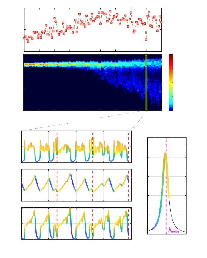
www.nature.com/scientificreports/
Figure 1. Process flow of the encoding of the input signal. M input samples {x (1) , . . . , x (M) } of dimension
N are queued on the columns of a matrix Xin. The dimension of each sample is then increased to Nv using
a connectivity matrix Win. A global offset u0 is applied to Win Xin to remove the negative values, and a
multiplicative scale factor α is applied. The resulting column values represent the input pump power (red curve)
u of each sample, which are sequentially injected at times tn = n(Nv �) at the input port of the MR (central
inset). Similarly, the values of the probe power upr (tn,i ) at times tn,i = n(Nv �) + i�, with i = {1, . . . , Nv }, define
the virtual nodes at the output of the Drop port of the MR.
The pump wavelength p is set with a small detuning p with respect to one of the resonance orders p,0
(pump resonance) of the MR. A second probe laser, at a constant power Ppr ≪ Pp , is injected into the same
port, and is tuned at a wavelength pr = pr,0 + pr , with a detuning pr with respect to the probe resonance
wavelength pr,0. We used | pr,0 − p,0 | = FSR, where FSR is the Free Spectral Range of the MR. In the rest of this
paper, we refer to p,0( pr,0) as the “cold” pump(probe) resonance, that is the resonance wavelength of the MR
in the linear operation regime, where all the nonlinear effects, which might affect the resonance frequency, are
neglected. As a consequence of light confinement in the MR, the pump intensity builds up, and TPA promotes
free carriers from the valence to the conduction band. This changes the refractive index of the material through
FCD, inducing a rigid blue shift of all the eigenfrequencies of the M R35. Concurrently, the round-trip loss is
increased by Free Carrier Absorption (FCA). Since u varies in time, the magnitude of the FCD shift changes
as well, and its dynamics is imprinted on the probe laser intensity at the output of the MR. The latter incoher-
ently transfers the input information from the pump to the probe beam. It is worth to note that the FCD shift
caused by TPA is two orders of magnitude higher than the Kerr shift (see supplementary material), and acts as
an effective intensity induced nonlinearity. The carrier lifetime τfc is much smaller than the thermal constant τth
R37. Therefore, when � ∼ τfc , the MR temperature variations T cannot follow the temporal profile of
of the M
the carrier concentration. Self heating effects due to carrier relaxation are smoothed to yield a steady state value
T . In this regime, the MR temperature does not participate to the reservoir dynamics, and only changes the
effective detuning p( pr ) of the pump(probe) resonance. However, as discussed in “Enhancing the reservoir
performance by mixing thermal and free carrier dynamics” section, this holds only at low input power. When the
average power is raised above a certain threshold, the MR starts to self-pulse35, and the temperature dynamics
impacts the processing capabilities of the nodes.
We can get an insight on the internal structure of the reservoir by assuming small perturbations of the input
power u(t) with respect to a reference value u(t) . Here, small means that the corresponding free carrier change
N − N around the reference value N induces variations of the transmitted pump/probe intensity which
are linear with N . As derived in the supplementary material, within this approximation the probe power upr
at the Drop port of the resonator is given by:
t − t−ξ t − t−ξ
upr (t) = c0 + c1 e
τ
fc
u2 (ξ )dξ + c2 e
τ
fc
u2 (ξ )upr (ξ )dξ , (1)
−∞ −∞
where the definitions of c0, c1 and c2 are provided in the supplementary material. The first contribution to the
virtual node state at time t is quadratic in the pump power u, and depends on the past inputs with weights that
exponentially decrease with time. This short term memory is of the order of ∼ 3 τfc , i.e., the time required by free
carriers to reach a steady state after an abrupt change of the pump power. The memory of this system is thus intrin-
sically nonlinear. This is because the input information x (n) is instantaneously (fs scale) transferred to carriers
through nonlinear absorption, temporarily processed from a slower (ns) dynamics, and subsequently imprinted
36
to the output probe.
Similarly to what is done in , one can approximate the integral in the
first term with a
m
k
discrete sum,−and � find the recursive virtual node relation upr (tn,i ) = �c1
2 m
k=0 η u(tn,i−k ) + η upr (tn,i−m )
where η = e (for simplicity, the second term in Eq. (1) has been neglected, but this does not alter our
τfc
conclusions). This highlights the type of connectivity between the virtual nodes of the reservoir, which are
organized in a chain-like topology: node upr (tn,i ) is coupled with its adjacent upr (tn,i−1 ) with a coupling strength
η. The latter exponentially decreases with the time separation, so the number of coupled nodes depends on . It
Scientific Reports | (2021) 11:15642 | https://doi.org/10.1038/s41598-021-94952-5 3
Vol.:(0123456789)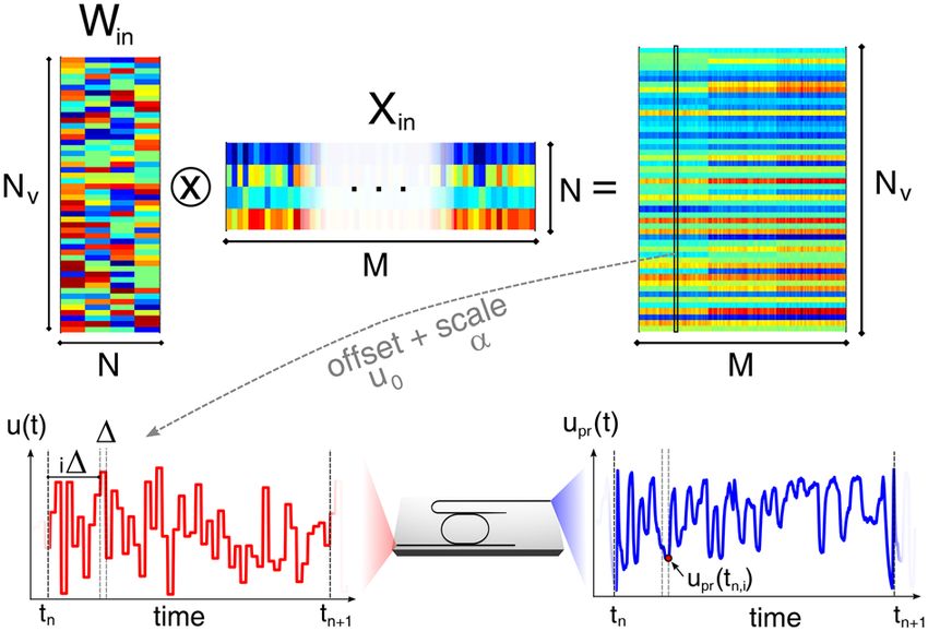
www.nature.com/scientificreports/
Figure 2. Sketch of the experimental setup. TLS = Tunable Laser Source, AWG = Arbitrary Waveform
Generator, EO mod. = Electro Optic modulator, FPC = Fiber Polarization Controller, VOA = Variable Optical
Attenuator, PD = Photodiode, EDFA = Erbium Doped Fiber Amplifier, BS = Beam Splitter, GC = Grating
Coupler, BPF = BandPass Filter, OSC = Oscilloscope. An enlarged view of the device layout and the main logical
steps which describe how the information is processed are shown in the bottom part of the figure. The intensity
modulated pump (red) and the CW probe (blue) are injected into the input GC. The incoherent transfer of
information from the pump to the probe occurs within the resonator (reservoir), where the different virtual
nodes (yellow dots) interact and process the input data. The probe exits from the Drop port, carrying the result
of the computation. Virtual nodes are sampled and sent into several linear classifiers, each trained to recognize a
specific class. The decision making process is based on a winner takes all scheme.
has been shown that an optimal value for is of the order of ∼ τ/5, where τ is the characteristic time response
of the nonlinear node9,36. We choose � ∼ τfc for our experiment, which is fast enough to prevent our device to
reach a steady state. The second term in Eq. (1) is a nonlinear coupling between virtual nodes. This term arises
from the the resonance shift induced by FCD (see supplementary material). The shift modifies the pump power
circulating in the MR, which in turn affects the carrier generation rate. As a result, a recursive relation between
these quantities is settled, for which the second term in Eq. (1) accounts for the leading term. When the change
in upr is no more linear with N − N due to large FCD induced resonance shifts, Eq. (1) loses validity and
the virtual node interaction becomes increasingly complex. The general structure of the network is however
maintained, with TPA and inter-node coupling providing nonlinearity, while carrier recombination a short term
memory to the reservoir. Virtual nodes upr (tn,i ) are sampled at the Drop port synchronously with the input, and
(1) (M) (k)
arranged into a state matrix X = [upr , . . . , upr ]T , where upr is the column vector collecting the Nv virtual nodes
corresponding to the k input sample x . The action of the reservoir is to project the initial set of predictors
th (k)
x (k) with corresponding observables y (k) (in general, a Q-dimensional vector) to a higher dimensional space
(k)
x (k) → upr where they ideally should be linearly separable. Then, the aim is to find a (Nv × Q) weight matrix
Wout which realizes Y = XWout , in which the observables are arranged in the M × Q matrix Y . We accomplish
this task by regularized least squares (Ridge regression), where the regularization parameter is determined by
a 5-fold cross v alidation38. The output of this procedure is a matrix W̃out which minimizes the regularized least
square error M k=1 ||(Y − W̃out X)|| + ||W̃out || . In case of supervised learning, as we deal in this paper, y
2 2 2 (k)
is a Q-dimensional binary variable, with 1s identifying the assignment category of x (k) and 0s elsewhere. Given
ỹ (k) and y k , the way decisions arehandled depends on the task, and will be treated separately in “Binary input:
1-bit delayed XOR” and “Analog input: Iris species recognition” sections.
Experimental realization
Our experimental apparatus is sketched in Fig. 2. The pump is a C-band, CW tunable laser (Pure Photonics)
which is intensity modulated by an electro-optic IQ modulator (IxBlue MXIQ-LN-30) to realize the desired input
pump waveform u(t). The modulator is driven by a 65 Gs Arbitrary Waveform Generator (AWG) from Keysight,
whose output is amplified by a high bandwidth amplification stage (IxBlue DR-AN-28-MO), providing the nec-
essary voltage swing of Vπ ∼ 7 V to exploit the full dynamic range of the modulator. In order to claim that the
nonlinear transformation on the input samples is solely coming from the MR, we did a pre-compensation of the
signal out of the AWG, which eliminates the cos2 dependence of the modulator intensity response with the applied
voltage. A tap of 10% is placed at the output of the modulator to monitor the input pump, which is detected by
Scientific Reports | (2021) 11:15642 | https://doi.org/10.1038/s41598-021-94952-5 4
Vol:.(1234567890)www.nature.com/scientificreports/
a) b) c)
Figure 3. (a) Examples of waveforms processed during the XOR task. The pump laser driving the input port
of the MR is shown in black, while the pump and probe outputs from the Drop port are respectively shown in
red and blue. (b) Bit Error Rate (BER) as a function of the bitrate for the 1-bit delayed XOR task. Black dots use
a predictor matrix X whose entries are sampled from the input pump power. Red and blue dots use respectively
predictors sampled from the pump and the probe traces at the Drop port of the MR. In all the three cases, the
average pump power is set to 3 dBm. (c) Bit Error Rate as a function of the average pump power for a fixed
bitrate of 20 Mbps. The insets show details of the probe waveform at the pump powers −10 dBm and 4 dBm.
a fast photodiode (Thorlabs DXM20AF). The pump is amplified to a fixed level of 20 dBm by an Erbium Doped
Optical Amplifier (EDFA, IPG Photonics) and the power regulated by an electronic Variable Optical Attenuation
(VIAVI mVOA-C1). A second CW probe laser (Pure Photonics) is combined with the pump before being injected
into the input port of the MR using a single mode fiber and a Grating Coupler (∼ 3.5 dB loss). The MR under
test has a racestrack shape, with a radius of 7 µm and a waveguide cross section of 450 nm × 220 nm. Two bus
waveguides are coupled to the straight sections of the MR, with a gap of 250 nm and a coupling length of 3 µm.
The device is described in great detail i n37. From the low-power transmission spectra recorded at the Through
port, we extracted an intrinsic quality factor (Q) of Qi = 1.11(8) × 105 and a loaded Q of QL = 6.5(2) × 103.
We use two adjacent resonance orders to resonantly couple the pump and probe laser, which have respectively
a cold resonance wavelength of ∼ 1549 nm and ∼ 1538 nm. Light at the output of the Drop port is amplified by
a second EDFA (Thorlabs), and a tunable band-pass filter (0.8 nm bandwidth) removes the spontaneous emis-
sion and directs the probe or the pump laser to the output photodiode (Thorlabs D400FC, 1 GHz bandwidth).
A 4 × 40 Gs oscilloscope (LeCroy SDA 816Zi-A) records the input pump waveform u(t) and the output probe
upr (t). Virtual nodes are sampled from upr (t) at times tn,i and queued to form the state matrix X . Training and
validation are performed off-line using Matlab.
Binary input: 1‑bit delayed XOR. The first task we tested is the 1-bit delayed XOR20. Given the virtual
(k)
node vector upr at time tk , the goal is to predict the result of the XOR operation between the bits x (k) and x (k−1).
The input variable can assume two values, 1 (full transmission of the modulator) and 0 (full extinction). In
this task, we use Nv = 3 virtual nodes, and the connectivity mask is simply a 3 × 1 column vector of 1s. This
implies that no mask is applied to the input data, so that u(tn,i (σ )) = x (n) θ (tn,i (σ )). We do not aim to use this
task as a benchmark, but to a give proof of concept demonstration of the architecture operation, which involves:
the nonlinear transformation of the inputs, the presence of a fading memory, and the ability to deal with binary
inputs. In this experiment, we fix the average power of the pump at the input to 3 dBm , which is sufficient to
trigger TPA and carrier generation, and its detuning to p = 60 pm . The pump intensity is modulated with
∼ 18 dB of extinction, and the input is a Pseudo Random Binary Sequence (PRBS) of bitrate B, which we varied
from 10 Mbps to 80 Mbps . The probe power is set to Ppr = −3 dBm , which is sufficiently low to not alter the
resonance shift imparted by the pump, and its detuning to pr = 60 pm. An example of waveforms at the input
and output of the MR for a bitrate of 30 Mbps are shown in Fig. 3(a). Whenever the input pump changes from
a low to an high state, a transient exponential decay is observed at the Drop port, which is due to the blue shift
of the resonance as a consequence of carrier generation and accumulation. The cold cavity detuning � p(pr) is
increased by FCD, determining a decrease of the transmittance, which also occurs for the probe output. The
opposite trend is observed, in the probe trace, during the transition from a high to a low state. Here, carrier
recombines and the detuning � p (pr) decreases, pulling the resonance back to the cold position. All the transient
phenomena occur at the characteristic timescale of τfc = 45 ns, i.e., the value of the carrier lifetime we measured
in one of our previous works37.
Virtual nodes are obtained by sampling these traces at 10 Gbps, smoothing them with a moving average filter
(10 points), and downsampling them at times � = (Nv B)−1. After smoothing, the Signal to Noise ratio (SNR)
increases from 18 dB (from the raw data acquisition) to ∼ 20 dB. The procedure for the estimation of the SNR is
detailed in the supplementary material. Figure 3(b) shows the Bit Error Rate (BER) as a function of the bitrate
for different predictor matrices X , whose entries are respectively populated by sampling the virtual node values
from the input pump intensity (black), the output pump power (red) and the output probe power (blue). To
Scientific Reports | (2021) 11:15642 | https://doi.org/10.1038/s41598-021-94952-5 5
Vol.:(0123456789)www.nature.com/scientificreports/
extract the BER, 6500 bits are used for training and 3500 for validation. Errorbars are obtained by partitioning
the validation set into 5 non-overlapping batches, over which the BER is evaluated. The error is estimated as
the standard deviation over the different batches. The output of the linear classifier Ỹ is digitized by applying
a threshold, which optimizes the BER at each bitrate. The XOR task is never solved by sampling virtual nodes
from the bare input pump. The average BER is ∼ 30% for all the bitrates. This agrees with the fact that the task
is not linearly separable and requires at least one bit of memory to be performed.
Virtual nodes sampled from the pump at the output of the Drop port improve the BER, which is however
still bounded above ∼ 5%. The reason behind this is that bits which are zero do not carry optical power, so these
virtual nodes are sampled from the background noise. This issue is solved by using the probe signal. Indeed,
error free operation is achieved for bitrates lower than 25 Mbps. Since we use 700 bits for each partition, error
free means that the actual BER is lower than 1.4 × 10⁻³. At higher rates, carriers are no more able to react suf-
ficiently fast to follow the pump power variations, so the BER increases. The ability to solve the delayed XOR
demonstrates the presence of memory and nonlinearity in the reservoir. This also illustrates that the use of a
probe beam is beneficial for tasks where the input is binary and with full modulation. It helps to improve the
separability of the r eservoir25. To investigate the influence of the input power on the BER, we fixed the bitrate
to 20 Mbps, and we changed the average input power of the pump Pp. The calculated BER is shown in Fig. 3(c).
The error rate is almost power-insensitive and equal to ∼ 25% for Pp < −4 dBm , while it drops below 1% at
Pp = 0 dBm. At Pp > 2 dBm, error-free operation is achieved. The low and high power insets shown in Fig. 3(c)
explain why the BER improves by increasing power. At Pp = −10 dBm, few carriers are generated, so the probe
is weakly perturbed from its original CW state and virtual nodes acquire a noisy flat distribution of values. At
Pp = 4 dBm, the FCD shift is source of more variability in the virtual nodes states, improving the input separa-
bility of the reservoir. We also averaged several traces at low power in order to compare the performance at the
same SNR of the ones at high power, but we only observed a minor improvement of the BER. This confirms that
the poor performance measured at low power is due to the reduced virtual node variability.
Analog input: Iris species recognition. The second task we addressed is the classification of the Iris
flowers, a popular toy-dataset in the field of machine learning34, and being so, not intended to be used as a
benchmark against other reservoir systems. Here, the goal is to classify a given Iris flower into one of the three
possible subspecies: Setosa, Versicolor and Verginica. The classification is based on four real inputs x , physically
corresponding to the length and width of the petals and sepals of the flower. All the four inputs are required to
solve the task, since the flowers can not be linearly classified on the basis of a single feature. Moreover, even by
using all the four inputs, only one species (Setosa) is linearly separable from the others, making the task non-
trivial. As described in “Principle of operation” section, the dimension of the original input space is increased
from 4 to Nv by implementing the transformation x → Win x , where the connectivity matrix Win has dimension
Nv × 4. An offset is applied to the transformed input to remove the negative values, and the result is scaled to
reach the desired target average power Pp. We tested different numbers of virtual nodes Nv = {10, 25, 50}, and
two values of time separation = {25, 50} ns. Each flower sample is sequentially encoded in the pump inten-
sity u(t) and injected into the input port of the MR. Different flowers are separated by a delay of δ = 100 ns,
during which the pump power is turned off to quench the carrier dynamics. This avoids undesired crosstalk of
information between neighbouring flowers, resetting the MR to the same initial conditions after each sample
injection. The original dataset contains 150 flowers, with an equal number of representatives of each class. Each
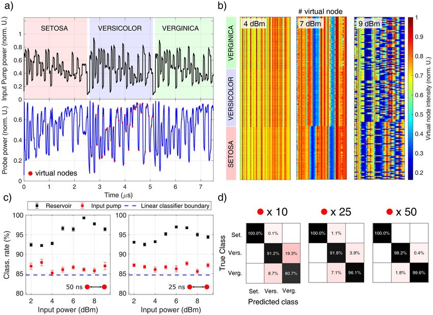
instance injected into the chip is randomly extracted from the dataset. Figure 4(a)(top panel) shows an example
of pump waveform at the input of the MR for three flower instances of different subspecies. Each is made by 50
steps, which corresponds to the virtual nodes. The low speed of operation allows to use the full resolution of
the digital to analog converter of the AWG (8 bit), imprinting on the optical power trace the fine details of each
flower sample. The associated probe waveform, after being processed by the MR reservoir, is shown in Fig. 4(a)
(bottom panel). With respect to the XOR task, where the input is binary, the multilevel excitation imparts a
richer dynamics on the output probe, which results in an enhanced variability between the virtual nodes. The
reservoir response to different flower samples is represented in the maps of Fig. 4(b), which shows the intensities
of the 50 virtual nodes for 189 flower instances (vertically stacked). In Fig. 4(c) we report the classification rate
for 20 Mbps and 40 Mbps as a function of the average input power. Categories are assigned by training multiple
linear classifiers, one for each subspecies, and decisions are made on the basis of a winner takes all s cheme9.
The best performance is obtained for 20 Mbps and a pump power of Pp = 7 dBm, yelding a classification rate
of (99.3 ± 0.2)%. In comparison, the classification rate obtained by sampling the virtual nodes from the input
pump is below 87%. This value is slightly above the theoretical limit of 84.66%, obtained by directly feeding the
input predictor matrix Win Xin into a linear classifier. This is probably due to some residual nonlinear distor-
tion in the electro-optic conversion. The rate of classification obtained by a single MR exceeds the accuracy
achieved by a more complex integrated system (three layered feed forward neural network)39, and has competi-
tive performance with respect to software based classification algorithms40 or compared to a complex-valued
perceptron, which has been recently implemented on a coherent photonic processor19. The classification rate in
Fig. 4(c) increases from low to high power, reaches a maximum at 7 dBm and then decreases for higher powers.
We can understand this trend by observing the virtual node intensity in the maps of Fig. 4(b). At low powers
( Pp = 4 dBm in Fig. 4b), the MR reservoir shows poor separability of the inputs, as witnessed by the quite flat
virtual node intensity distribution observed both within the same flower (horizontal lines) and between different
subspecies (vertical lines). As discussed for the XOR task, this is related to the weak perturbations imprinted on
the CW probe from the pump intensity at low powers. At the highest classification rate of Pp = 7 dBm (Fig. 4b),
the virtual node distribution is richer, with a relative variation that can exceed 70% (see Fig. 4b at Pp = 7 dBm).
We also observe the creation of two bands, where the virtual node intensity is around the 35% of its maximum
Scientific Reports | (2021) 11:15642 | https://doi.org/10.1038/s41598-021-94952-5 6
Vol:.(1234567890)www.nature.com/scientificreports/
Figure 4. (a) Examples of waveforms of the input pump (top panel, in black) and of the probe at the output of
the MR (bottom panel, in blue) for Nv = 50 and a bitrate of 20 Mbps. Different background colours highlight
the subspecies of the flower. Virtual nodes sampled from the probe trace are indicated with red dots on the
central band. (b) Maps of the (normalized) intensity of the different virtual nodes (Nv = 50, bitrate 20 Mbps)
sampled from the output probe, acquired at the pump powers of 4 dBm (left), 7 dBm (center), and 9 dBm (right).
These are 189 flower samples vertically stacked in each map. Even if they are randomly injected at the input port
during the training and test phase, they are shown grouped together in the three subspecies, as indicated by the
labels on the left. This highlights the distinction between the classes. (c) Classification rate as a function of the
average input power of the pump for Nv = 50 and bitrates of 20 Mbps (left) and 40 Mbps (right). Black scatters
use virtual nodes sampled from the output probe while red scatters from the input pump. The dashed blue line
is the lower bound in the classification rate obtained by feeding the input samples into a linear classifier, without
electro-optic conversion. (d) Confusion charts for a MR reservoir which uses 10 (left), 25 (center), and 50
(right) virtual nodes. The bitrate is 20 Mbps.
value. As discussed in “Enhancing the reservoir performance by mixing thermal and free carrier dynamics” sec-
tion, these form as a consequence of the interplay between thermal and free carrier dispersion. At high power
( Pp = 9 dBm in Fig. 4b), multiple bands of low transmittivity are formed, which lack synchronization with the
rate of flower injection. Within the bands the MR is off resonance, hence the information can not be efficiently
imprinted from the pump to the probe, effectively “burning” these virtual nodes from the reservoir. This explains
the drop in the classification accuracy at high powers.
The net flower classification rate can be calculated as (Nv � + δ)−1, which for Nv = 50 and = 50 ns, i.e.,
the configuration showing the best accuracy, is 0.38 MHz . We tried to scale down to Nv = 25 and Nv = 10 in
order to improve the speed of operation, but as shown by the confusion charts in Fig. 4(d), the classification
accuracy drops to (93.6 ± 0.3)% for Nv = 25 and (89.2 ± 0.2)%) for Nv = 10. We did not observe any significant
improvement by scaling up to Nv = 100.
Enhancing the reservoir performance by mixing thermal and free carrier dynamics. In order to
explain the behavior of the classification rate as a function of the input pump power in Fig. 4(c), we performed
numerical simulations. They are based on the theoretical model o f37. Specifically, we computed the time evolu-
tion of the complex field in the MR, including TPA, FCA, FCD and the thermo optic dispersion (TOE). When-
ever possibile, the parameters are taken from the experiment. A more comprehensive description of the model
Scientific Reports | (2021) 11:15642 | https://doi.org/10.1038/s41598-021-94952-5 7
Vol.:(0123456789)www.nature.com/scientificreports/
Figure 5. (a) Top: numerical simulation of the Iris dataset classification rate as a function of the input power.
Bottom: probability distribution of the virtual node detuning as function of the input pump power. (b)
Simulated probe power at the Drop port of the MR (top), temperature variation (middle) and free carrier
concentration for Pp = 9 dBm. The red dashed lines mark the injection times of three different flower samples.
The color code indicates the instantaneous detuning of the probe, whose relation with the Drop intensity is
shown in panel (c). (c) Normalized intensity at the Drop port of the MR as a function of wavelength. The dashed
line marks the wavelength of the probe laser. The color code is used to label the instantaneous detuning of the
time traces in panel (b).
can be found in37. We fix the number of virtual nodes to 50, the bit rate to 20 MHz and the quenching time to
δ = 100 ns.
The top panel in Fig. 5(a) shows the simulated classification rate as a function of the input power, estimated
from the whole Iris dataset (150 flowers). We add white noise to the simulated output of the MR to set the SNR
to 18 dB, which is comparable to the one of the experiment (the latter monotonically decreases from ∼ 25 dB
at 2 dBm of input Pump power to ∼ 17 dB at 9 dBm, see supplementary material for details). Each point is
the result of an average over 1000 realizations. We notice a very good agreement with the experimental data
in Fig. 4(c), with a maximum of classification occurring around 7 dBm. We investigate the origin of this trend
starting from the color map reported in the bottom panel of Fig. 5(a). Here, for each input power, we calculate
the probability that a virtual node is sampled at the probe resonance detuning from the cold cavity condi-
tion. At low power, all virtual nodes are sampled around the cold resonance detuning, which in our case lies at
= 60 pm. As we raise the input power up to about 5 dBm, FCD shifts the resonance frequency towards the
blue, further increasing the initial detuning. Starting from 6 dBm, we observe that the variance increases, and
that there is a small probability to sample virtual nodes at negative detunings. For Pp > 6 dBm, the distribution
Scientific Reports | (2021) 11:15642 | https://doi.org/10.1038/s41598-021-94952-5 8
Vol:.(1234567890)www.nature.com/scientificreports/
is bimodal, i.e, nodes are concentrated around two bands: a narrow one at positive and a broad one at nega-
tive . This is a signature that the temporal evolution is not only related to free carriers, where the temperature
acts as a constant background. In fact, at these powers, we are entering a regime where carriers and temperature
dynamics mix together. This is shown in the panels of Fig. 5(b), which refer to Pp = 9 dBm . Here we report,
as a function of time, the output power of the probe (top), the temperature difference between the MR and its
surroundings (middle), and the free carrier concentration (bottom) for three consecutive flower samples (the
injection times are marked with red dashed lines). The color code indicates the instantaneous detuning of the
probe, whose relation with the Drop intensity is shown in Fig. 5(c). When a flower sample is injected, the tem-
perature of the MR increases, but at low powers TOE is counteracted by FCD. At high power TOE prevails, and
the wavelength detuning of the cavity can eventually become negative. When this occurs, a positive feedback is
established between the decrease of the carrier concentration and the decrease of MR energy. This corresponds
to the transition from the high power stability branch of the carrier bistability curve to the one at low p ower41.
35
After the transition, the MR lies off r esonance . The detuning is now negative due to the residual thermo optic
shift. This originates the bands of low transmittivity in Fig. 4(b) and in Fig. 5(b). Virtual nodes sampled within
these bands form the second broad peak in the probability distribution in Fig. 5(a). As the MR cools down, the
resonance moves towards the pump(probe) wavelength, gradually increasing the probe signal. A transition
from the low power stability branch of the carrier bistability curve to the one at high power restores the initial
conditions, so that virtual nodes are no more sampled within the band. This interplay of thermal and free carrier
effects would generate cavity self-pulsing in case of CW input powers35. It turns out that, for a limited range of
powers centered around 7 dBm, the presence of the bands increases the classification rate. This finds explanation
in the enhanced variability that the virtual nodes values assume. Indeed, in this regime, they efficiently sample
all the probe resonance. Moreover, quenching the MR for δ = 100 ns allows to reset the initial conditions for the
temperature and the carrier population between consecutive flower samples, creating bands always in the same
time slot (see Fig. 4(b), Pp = 7 dBm). If the power is increased above 7 dBm, bands get wider in time and many
of them form within the same flower sample. In these conditions, a large number of virtual nodes are sampled
within bands, where the cavity lies off resonance and hence no information can be transferred from the pump
to the probe beam. Furthermore, the quenching time is no more sufficient to reset the initial conditions, so as
bands form at random times, turning the probe output to chaotic (see Fig. 4(b), Pp = 9 dBm)42.
Discussion
In the above sections, we demonstrated the use of a single integrated MR as a reservoir, in which the core com-
puting power is provided by the complex coupled dynamics of free carriers, TPA and temperature. The overall
power consumption is estimated to be around 1500 W , and is distributed as follows: 60 W for the Pump and
Probe lasers, 5 W for the electrical amplifiers, 180 W for the AWG, 40 W for the optical amplifiers, 1000 W for the
oscilloscope and 200 W for the laptop. This is comparable to the value of 1300 W reported in a recent work on a
silica chip29, and is expected to not significantly differ from the one of more advanced photonic c lassifiers8,9,43,
since most of the power consumption arises from the electronics used for data acquisition, control and post
processing, rather than from the optical components. The architecture is proof of concept and suffers from
an unusually slow carrier recombination time. As such, it faces limitations in terms of speed, dimensionality,
power consumption and performance, which are nevertheless not of fundamental origin. We now outline how
to improve these metrics with modest technological effort. First, to increase the dimensionality, the MR can be
used as a building block to form more advanced spatial topologies, i.e. matrices/arrays of MR. As an example,
using resonators with a moderately high Q factor of 6.5 × 10⁴ , a network made by 10 MR can accommodate
500 virtual nodes and operates with 5 mW of power. Small sequences of coupled resonators have shown very
complex dynamics under thermal and free carrier nonlinearities42, which suggests that the same performance
could be obtained with less virtual nodes, hence increasing the speed of operation. Additionally, a narrower cavity
linewidth enhances the sensitivity of the resonator to small resonance perturbations, decreasing the input power
needed to trigger free carrier effects. Higher degrees of complexity and computational power could be realized
by multiplexing several spatial inputs44 and by coherently combining them on chip using linear optical elements,
such as arrays of Mach-Zehnder interferometers arranged in a universal scheme18. This hybrid spatio-temporal
architecture combines a simple hardware implementation, typical of delayed nodes RC, with the compactness
of a silicon photonic chip. Second, to increase the speed of operation and reduce the power consumption, the
intrinsic time response of the RC can be improved by reducing the carrier lifetime. Indeed, our device shows
a recombination time which is almost two orders of magnitude higher than the ones commonly reported in
literature31. Several factors may hinder the recombination process, such as a small surface trap density or the
presence of trap states located below the Fermi level of the semiconductor45. A prior analysis performed on the
same device rules out the latter hypothesis37. We can then speculate that the long carrier lifetime is associated
to a small trap density, which could correspond to a well passivated waveguide surface. It is possible to push the
lifetime down to tens of ps by embedding carrier depletion modulators within the M R33. The aggregate processing
43,46
speed can be also improved by adopting wavelength-division multiplexing . This would require to use multiple
pump lasers whose wavelenghts are matched to the different resonance orders of the MR. Different virtual nodes
can be encoded into distinct wavelengths and simultaneously injected into the reservoir. It is worth to note that
this is not equivalent to operate several independent reservoirs in parallel. Indeed, since the carrier population
interacts with all the optical channels, they become coupled (second term in Eq. (1))47, and additional virtual
node interaction is expected from Cross Photon Absorption. In this sense, the number of Multiply-Accumulate
(MAC) operations will not generally scale with the number of wavelengths.
Another aspect of concern is the memory capacity. Since our device lacks of a delay loop, the memory is
provided by carrier relaxation, and is of short term. As shown in “Principle of operation” section, the input is
Scientific Reports | (2021) 11:15642 | https://doi.org/10.1038/s41598-021-94952-5 9
Vol.:(0123456789)www.nature.com/scientificreports/
convoluted with a slow exponential decay, which means that the virtual node coupling only extends over the first
few neighbours. We can anyway compensate the absence of a long-range coupling by encoding the memory over
past samples in the input layer. Indeed, it has been shown that a delay loop reservoir whose feedback has been
removed can still be effective in time prediction tasks, provided that memory over past samples is given at the
input21,48. To see how this can be implemented in our scheme, we consider the discrete time version of Eq. (1), and
(n)
express the pump field as u(tn,i ) = N k=1 Wik xk , which gives the following probe amplitude at the output layer:
− k� (n)
τ
Wi−k,q Wi−k,q′ rq,q′ xq(n) xq′ + O upr
upr (tn,i ) ∼ e fc
(2)
k,q,q′
where the sums over q and q′ run over all the components of the nth input sample, while rq,q′ = 1 if q = q′ and
rq,q′ = 2 if q = q′ . This is equivalent to operate N sample and hold circuits, each applying a different mask
Wj = [Win ]j ((j = 1, N) where [Win ]j denotes the jth column of Win ) to separate inputs xj . The outputs of the
N circuits are then multiplexed in the same input port to excite the nonlinear node. In time series prediction
(n) (n)
tasks, the xq can be the values of the series iin (t) sampled q bits ahead in time, i.e., xq = iin ((n − q)T), where
q runs over all the past samples which are relevant to perform predictions. The approach unifies the concepts of
reservoirs and extreme learning m achines48. Compared to delayed loop reservoirs, the overhead is that several
delayed copies of the same input series and a combination stage are required. This is not of particular concern
since in most of the cases an electro-optic conversion is involved to shape the input series from a CW optical
input, so all the described pre-processing steps can be done in the electronic domain using a combination of
delay lines and fan-in(out) circuits. An alternative strategy is to use different wavelength channels to encode the
delayed copies, and to broadcast them into the same spatial mode using an on-chip wavelength multiplexer, as
an Arrayed Waveguide Grating or a Mach Zehnder interleaver. As a last remark, we point that the presence of a
delay loop may not always be desired. While it is certainly beneficial for tasks requiring a long term memory, in
classification tasks this introduces crosstalk among different objects, which deteriorates the input separability.
Conclusions
In this work, we have experimentally shown a time multiplexed architecture which uses a single integrated
MR as a substrate for RC. We encode the input layer in the temporal evolution of the intensity of a pump laser.
When this is resonantly coupled to the MR, the information is transferred to a secondary probe laser, which is
tuned on an adjacent resonance order. The transfer is enabled by TPA, which generates a free carrier dynamics
that is imprinted on the probe laser by FCD. We train the reservoir to perform some proof of concept tasks by
using regularized linear regression. We experimentally demonstrate that the system can handle problems with
binary and analog inputs. We have shown that the MR solves the 1-bit delayed XOR task with a minimum BER
of 1.4 × 10⁻³ for bitrates up to 30 MHz . This result is obtained by only exploiting the nonlinear free carrier
dynamics. As a second step, we have shown that the system can solve the analog task of the classification of the
Iris dataset.
We demonstrated a maximum classification rate of (99.3 ± 0.2)% at a rate of 0.38 MHz, using an average power
of 7 dBm at the input of the MR. In this regime, the thermal and the free carrier dynamics are strongly coupled.
This feature enhances the separability properties of the reservoir, by adding more variability to the virtual node
distribution. The optimal performance is found across the edge between a stable and a self-pulsing regime, which
agrees with the predictions of numerical simulations.
To the best of the author’s knowledge, this is the first experimental demonstration of RC using a silicon MR.
We envisaged several future developments and engineering solutions, all leveraging on silicon photonics. This
will open the doors to the realization of a wide range of hybrid spatio-temporal reservoirs offering increased
computational complexity.
Received: 11 June 2021; Accepted: 16 July 2021
References
1. Russakovsky, O. et al. Imagenet large scale visual recognition challenge. Int. J. Comput. Vis 115, 211–252 (2015).
2. Buetti-Dinh, A. et al. Deep neural networks outperform human experts capacity in characterizing bioleaching bacterial biofilm
composition. Biotechnol. Rep. 22, e00321 (2019).
3. Silver, D. et al. Mastering the game of go with deep neural networks and tree search. Nature 529, 484–489 (2016).
4. Assael, Y. M., Shillingford, B., Whiteson, S. & De Freitas, N. Lipnet: End-to-end sentence-level lipreading. arXiv preprint: arXiv:
1611.01599 (2016).
5. Jaeger, H. The echo state approach to analysing and training recurrent neural networks-with an erratum note. Bonn, Germany:
German National Research Center for Information Technology GMD Technical Report 148, 13 (2001).
6. Jaeger, H. & Haas, H. Harnessing nonlinearity: Predicting chaotic systems and saving energy in wireless communication. Science
304, 78–80 (2004).
7. Maass, W. & Markram, H. On the computational power of circuits of spiking neurons. J. Comput. Syst. Sci. 69, 593–616 (2004).
8. Vinckier, Q. et al. High-performance photonic reservoir computer based on a coherently driven passive cavity. Optica 2, 438–446
(2015).
9. Larger, L. et al. High-speed photonic reservoir computing using a time-delay-based architecture: Million words per second clas-
sification. Phys. Rev. X 7, 011015 (2017).
10. Appeltant, L., Van der Sande, G., Danckaert, J. & Fischer, I. Constructing optimized binary masks for reservoir computing with
delay systems. Sci. Rep. 4, 3629 (2014).
11. Antonik, P., Marsal, N. & Rontani, D. Large-scale spatiotemporal photonic reservoir computer for image classification. IEEE J. Sel.
Top. Quantum Electron. 26, 1–12 (2019).
Scientific Reports | (2021) 11:15642 | https://doi.org/10.1038/s41598-021-94952-5 10
Vol:.(1234567890)www.nature.com/scientificreports/
12. Vandoorne, K., Dambre, J., Verstraeten, D., Schrauwen, B. & Bienstman, P. Parallel reservoir computing using optical amplifiers.
IEEE Trans. Neural Netw. 22, 1469–1481 (2011).
13. Bueno, J. et al. Reinforcement learning in a large-scale photonic recurrent neural network. Optica 5, 756–760 (2018).
14. Paquot, Y. et al. Optoelectronic reservoir computing.. Sci. Rep. 2, 287 (2012).
15. Takano, K. et al. Compact reservoir computing with a photonic integrated circuit. Opt. Express 26, 29424–29439 (2018).
16. Vatin, J., Rontani, D. & Sciamanna, M. Experimental reservoir computing using vcsel polarization dynamics. Opt. Express 27,
18579–18584 (2019).
17. Zečević, N. et al. A 3d photonic-electronic integrated transponder aggregator with 48 × 16 heater control cells. IEEE Photonics
Technol. Lett. 30, 681–684 (2018).
18. Yichen, S. et al. Deep learning with coherent nanophotonic circuits. Nat. Photonics 11, 441–446 (2017).
19. Zhang, H. et al. An optical neural chip for implementing complex-valued neural network. Nat. Commun. 12, 1–11 (2021).
20. Vandoorne, K. et al. Experimental demonstration of reservoir computing on a silicon photonics chip. Nat. Commun. 5, 3541 (2014).
21. Harkhoe, K., Verschaffelt, G., Katumba, A., Bienstman, P. & der Sande, G. V. Demonstrating delay-based reservoir computing
using a compact photonic integrated chip. Opt. Express 28, 3086–3096 (2020).
22. Katumba, A., Yin, X., Dambre, J. & Bienstman, P. A neuromorphic silicon photonics nonlinear equalizer for optical communica-
tions with intensity modulation and direct detection. J. Lightw. Technol. 37, 2232–2239 (2019).
23. Laporte, F., Katumba, A., Dambre, J. & Bienstman, P. Numerical demonstration of neuromorphic computing with photonic crystal
cavities. Opt. Express 26, 7955–7964 (2018).
24. Denis-Le Coarer, F. et al. All-optical reservoir computing on a photonic chip using silicon-based ring resonators. IEEE J. Sel. Top.
Quantum Electron. 24, 1–8 (2018).
25. Mesaritakis, C., Papataxiarhis, V. & Syvridis, D. Micro ring resonators as building blocks for an all-optical high-speed reservoir-
computing bit-pattern-recognition system. J. Opt. Soc. Am. B 30, 3048–3055 (2013).
26. Mesaritakis, C., Bogris, A., Kapsalis, A. & Syvridis, D. High-speed all-optical pattern recognition of dispersive fourier images
through a photonic reservoir computing subsystem. Opt. Lett. 40, 3416–3419 (2015).
27. Katumba, A. et al. Low-loss photonic reservoir computing with multimode photonic integrated circuits. Sci. Rep. 8, 1–10 (2018).
28. Zhang, H. et al. Integrated photonic reservoir computing based on hierarchical time-multiplexing structure. Opt. Express 22,
31356–31370 (2014).
29. Nakajima, M., Tanaka, K. & Hashimoto, T. Scalable reservoir computing on coherent linear photonic processor. Commun. Phys.
4, 1–12 (2021).
30. Bogris, A., Mesaritakis, C., Deligiannidis, S. & Li, P. Fabry-perot lasers as enablers for parallel reservoir computing. IEEE J. Sel.
Top. Quantum Electron. 27, 1–7 (2021).
31. Xu, Q. & Lipson, M. Carrier-induced optical bistability in silicon ring resonators. Opt. Lett. 31, 341–343 (2006).
32. Wright, N. et al. Free carrier lifetime modification for silicon waveguide based devices. Opt. Express 16, 19779–19784 (2008).
33. Turner-Foster, A. C. et al. Ultrashort free-carrier lifetime in low-loss silicon nanowaveguides. Opt. Express 18, 3582–3591 (2010).
34. Fisher, R. A. The use of multiple measurements in taxonomic problems. Ann. Eugenics 7, 179–188 (1936).
35. Johnson, T. J., Borselli, M. & Painter, O. Self-induced optical modulation of the transmission through a high-q silicon microdisk
resonator. Opt. Express 14, 817–831 (2006).
36. Appeltant, L. Reservoir computing based on delay-dynamical systems. These de Doctorat, Vrije Universiteit Brussel/Universitat
de les Illes Balears (2012).
37. Borghi, M., Bazzanella, D., Mancinelli, M. & Pavesi, L. On the modeling of thermal and free carrier nonlinearities in silicon-on-
insulator microring resonators. Opt. Express 29, 4363–4377 (2021).
38. Tikhonov, A. N., Goncharsky, A., Stepanov, V. & Yagola, A. G. Numerical methods for the solution of ill-posed problems Vol. 328
(Springer, Berlin, 2013).
39. Shi, B., Calabretta, N. & Stabile, R. Image classification with a 3-layer soa-based photonic integrated neural network. In 2019
24th OptoElectronics and Communications Conference (OECC) and 2019 International Conference on Photonics in Switching and
Computing (PSC), 1–3 (2019).
40. Pinto, J. P., Kelur, S. & Shetty, J. Iris flower species identification using machine learning approach. In 2018 4th International
Conference for Convergence in Technology (I2CT), 1–4 (IEEE, 2018).
41. Zhang, L. et al. Multibistability and self-pulsation in nonlinear high-q silicon microring resonators considering thermo-optical
effect. Phys. Rev. A 87, 053805 (2013).
42. Mancinelli, M., Borghi, M., Ramiro-Manzano, F., Fedeli, J. & Pavesi, L. Chaotic dynamics in coupled resonator sequences. Opt.
Express 22, 14505–14516 (2014).
43. Xu, X. et al. 11 tops photonic convolutional accelerator for optical neural networks. Nature 589, 44–51 (2021).
44. Katumba, A., Freiberger, M., Bienstman, P. & Dambre, J. A multiple-input strategy to efficient integrated photonic reservoir com-
puting. Cogn. Comput. 9, 307–314 (2017).
45. Aldaya, I. et al. Nonlinear carrier dynamics in silicon nano-waveguides. Optica 4, 1219–1227 (2017).
46. Xu, S., Wang, J. & Zou, W. Optical patching scheme for optical convolutional neural networks based on wavelength-division
multiplexing and optical delay lines. Opt. Lett. 45, 3689–3692 (2020).
47. Harkhoe, K. & Van der Sande, G. Delay-based reservoir computing using multimode semiconductor lasers: Exploiting the rich
carrier dynamics. IEEE J. Sel. Top. Quantum Electron. 25, 1–9 (2019).
48. Ortín, S. et al. A unified framework for reservoir computing and extreme learning machines based on a single time-delayed neuron.
Sci. Rep. 5, 14945 (2015).
Acknowledgements
This project has received funding from the European Research Council (ERC) under the European Union’s
Horizon 2020 research and innovation programme (Grant Agreement No. 788793, BACKUP), and from the
MIUR under the project PRIN PELM (20177 PSCKT). The authors acknowledge Dr. Mattia Mancinelli and Mr.
Davide Bazzanella for the technical support in the experiment and the fruitful discussions.
Author contributions
M.B. conceived the idea of the experiment. M.B. and S.B. performed the measurements and processed the data.
S.B. performed the numerical simulations. L.P. supervised the work. All the authors contributed to the discus-
sions and wrote the manuscript.
Competing interests
The authors declare no competing interests.
Scientific Reports | (2021) 11:15642 | https://doi.org/10.1038/s41598-021-94952-5 11
Vol.:(0123456789)You can also read