Set-point optimization in wind farms to mitigate effects of flow blockage induced by atmospheric gravity waves - WES
←
→
Page content transcription
If your browser does not render page correctly, please read the page content below
Wind Energ. Sci., 6, 247–271, 2021
https://doi.org/10.5194/wes-6-247-2021
© Author(s) 2021. This work is distributed under
the Creative Commons Attribution 4.0 License.

       Set-point optimization in wind farms to mitigate effects of
         flow blockage induced by atmospheric gravity waves
                                              Luca Lanzilao and Johan Meyers
            Department of Mechanical Engineering, KU Leuven, Celestijnenlaan 300 A, 3001 Leuven, Belgium
                               Correspondence: Luca Lanzilao (luca.lanzilao@kuleuven.be)

                                     Received: 23 April 2020 – Discussion started: 8 May 2020
                      Revised: 18 December 2020 – Accepted: 24 December 2020 – Published: 5 February 2021

       Abstract. Recently, it has been shown that flow blockage in large wind farms may lift up the top of the bound-
       ary layer, thereby triggering atmospheric gravity waves in the inversion layer and in the free atmosphere. These
       waves impose significant pressure gradients in the boundary layer, causing detrimental consequences in terms of
       a farm’s efficiency. In the current study, we investigate the idea of controlling the wind farm in order to mitigate
       the efficiency drop due to wind-farm-induced gravity waves and blockage. The analysis is performed using a fast
       boundary layer model which divides the vertical structure of the atmosphere into three layers. The wind-farm
       drag force is applied over the whole wind-farm area in the lowest layer and is directly proportional to the wind-
       farm thrust set-point distribution. We implement an optimization model in order to derive the thrust-coefficient
       distribution, which maximizes the wind-farm energy extraction. We use a continuous adjoint method to effi-
       ciently compute gradients for the optimization algorithm, which is based on a quasi-Newton method. Power
       gains are evaluated with respect to a reference thrust-coefficient distribution based on the Betz–Joukowsky set
       point. We consider thrust coefficients that can change in space, as well as in time, i.e. considering time-periodic
       signals. However, in all our optimization results, we find that optimal thrust-coefficient distributions are steady;
       any time-periodic distribution is less optimal. The (steady) optimal thrust-coefficient distribution is inversely re-
       lated to the vertical displacement of the boundary layer. Hence, it assumes a sinusoidal behaviour in the stream-
       wise direction in subcritical flow conditions, whereas it becomes a U-shaped curve when the flow is supercritical.
       The sensitivity of the power gain to the atmospheric state is studied using the developed optimization tool for
       almost 2000 different atmospheric states. Overall, power gains above 4 % were observed for 77 % of the cases
       with peaks up to 14 % for weakly stratified atmospheres in critical flow regimes.

1   Introduction                                                       In a stable atmosphere, an air parcel which is vertically
                                                                    perturbed will have the tendency to fall back to its origi-
Today, it is well known that turbines strongly interact when        nal position. In such a case, an oscillation is initiated that
clustered together in large arrays, increasing the momen-           is driven by gravity and inertia; this is called a gravity wave.
tum deficit in the lowest region of the atmospheric boundary        Mountains are examples of orographic obstacles that trigger
layer (ABL). These turbine–turbine interactions, such as re-        vertical flow displacement and consequently gravity waves
duced wind speed and increased turbulence intensity, occur          (Smith, 1980). The drag force exerted by the mountain is
within the wind-farm area and can lead to detrimental con-          usually transported upward by these waves. At the point of
sequences in terms of a farm’s efficiency (Barthelmie et al.,       breakdown, the drag force is released in the upper levels of
2010). However, it has been recently discovered that non-           the atmosphere, causing a slowdown of the large-scale flow
local effects such as gravity waves may also have strong im-        (Eliassen and Palm, 1960; Durran, 1990). Moreover, when
plications on the wind-farm energy extraction (Allaerts and         air is lifted in a stable atmosphere, a cold anomaly is created,
Meyers, 2018, 2019).                                                which induces horizontal pressure gradients (Smith, 2010).

Published by Copernicus Publications on behalf of the European Academy of Wind Energy e.V.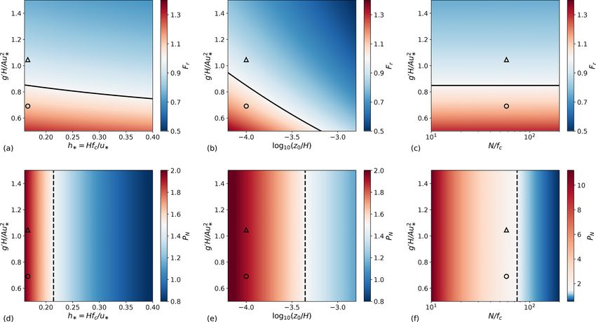
248                     L. Lanzilao and J. Meyers: Set-point optimization in wind farms to mitigate effects of flow blockage

   In a wind farm, the upward displacement of the bound-           strongly stratified atmospheres decrease the turbine power
ary layer, caused by diverging fluid streamlines due to flow       output up to 35 % with respect to the weakly stratified cases.
deceleration by the turbines, can trigger gravity waves in         Wind-farm flow blockage was also detected in field measure-
the stable free atmosphere above the boundary layer as well        ments. Wind speed data taken before and after the placement
(Smith, 2010; Allaerts and Meyers, 2017). As a result, an          of three wind farms showed that there was a reduction in
adverse pressure gradient develops in the induction region         wind speed of about 3 % in the induction region of each wind
of the wind farm, which slows down the wind-farm inflow            farm after turbines were installed (Bleeg et al., 2018).
velocity (Allaerts and Meyers, 2018). The size of this re-            In the last decades, a considerable amount of research has
gion scales with the length of the farm. This phenomenon           focused on wind-farm control strategies that allow the max-
is one possible cause of flow blockage. Note that it differs       imization of the farm power output. We refer to Kheirabadi
from classical hydrodynamic blockage caused by the turbine         and Nagamune (2019) for a recent comprehensive overview.
induction, which typically scales with the turbine rotor di-       However, earlier studies all focus on influencing wake dy-
ameter and which has also been studied recently in much            namics and wake mixing, which occur at a much smaller
detail (Bleeg et al., 2018; Segalini and Dahlberg, 2019).          scale than wind-farm-induced gravity waves, to improve
The goal of the current study is to determine a wind-farm          power extraction in waked turbines. Important control mech-
thrust-coefficient distribution that minimizes the gravity-        anisms include wake redirection (by yawing and tilting of the
wave-induced blockage effects, maximizing the flow wind            turbine), and turbine de-rating strategies. Control actions that
speed and therefore the power production. Moreover, we in-         influence wind-farm physics on a much larger scale, such as
vestigate the impact of different atmospheric conditions on        self-induced gravity waves, have not been explored to date.
the optimal thrust-coefficient distribution and corresponding         In the current work, we concentrate on using wind-farm
power gains.                                                       control to alter/improve the interaction between the wind
   Gravity waves have been related to flows over mountains         farm and its self-induced gravity-wave system. To this end,
for a long time (Queney, 1948). However, the cumulated             we use the fast boundary-layer model proposed by Allaerts
blockage effect induced by the wind farm in the induction          and Meyers (2019), which divides the vertical structure of
region was associated with wind-farm-induced gravity waves         the atmosphere into three layers (from here on named the
only in recent years. In the pioneering work of Smith (2010),      three-layer model in the paper), and we reformulate it as
a quasi-analytical model of atmospheric response to wind-          an optimization problem. The objective function is defined
farm drag was used for modelling gravity-wave excitation           as the wind-farm energy extracted over a time period T ,
due to diverging streamlines above the wind-farm area. Re-         while the constraints are the model equations plus a box con-
sults have shown that gravity-wave excitation is strongly de-      straint for the wind-farm thrust set-point distribution CT (x,
pendent upon the height of the boundary layer and the sta-         y, t). Note that we do not use the tip-speed ratio and/or
bility of the atmosphere aloft. Later, a fast boundary-layer       the pitch angle distribution as control parameters. Instead,
model was proposed by Allaerts and Meyers (2019), who              we directly control the thrust set-point distribution. In fact,
highlighted the crucial role of the inversion layer in determin-   the former approach would not add further insight into the
ing gravity-wave patterns. The authors also used this model        study performed in the current manuscript. The model equa-
for an annual energy production study of the Belgian–Dutch         tions are derived following the theory for interacting grav-
offshore wind-farm cluster, showing that the annual energy         ity waves and boundary layers developed by Smith et al.
loss due to the effect of self-induced gravity waves might be      (2006) and Smith (2007, 2010). Consequently, the optimal
on the order of 4 % to 6 % (Allaerts et al., 2018).                thrust-coefficient distribution computed using the optimiza-
   Gravity waves were also observed in mesoscale and large-        tion formulation of the three-layer model takes into account
eddy simulation (LES) models. Fitch et al. (2012) and Volker       the effects of self-induced gravity waves. Hence, we investi-
(2014) proposed two different wind-farm parameterizations          gate whether it is possible to mitigate gravity-wave-induced
for the Weather Research and Forecasting model (WRF).              blockage effects by varying the thrust set-point distribution
Wind-farm-induced gravity waves were observed in both              within the wind-farm area.
cases, causing flow deceleration several kilometres upstream          The remainder of this paper is formulated as follows. The
of the farm. Allaerts and Meyers (2017, 2018) have investi-        three-layer model and its optimization formulation are in-
gated the interaction between an “infinitely” wide wind farm       troduced in Sect. 2. Next, Sect. 3 describes the numerical
and both a conventionally neutral and stable boundary layer        setup, wind-farm layout and atmospheric state. Thereafter,
in typical offshore conditions in a LES framework. They            Sect. 4 presents optimization results. The optimal thrust set-
found that for low ABL heights, gravity waves induce strong        point distributions obtained in two different flow cases are
pressure gradients and play an important role in the distribu-     discussed in Sect. 4.1. The sensitivity of the power gain to
tion of the kinetic energy within the farm. Wu and Porté-Agel      the atmospheric state is carried out in Sect. 4.2. Finally, con-
(2017) considered a large finite-size wind farm operating in       clusions and suggestions for further research are given in
a conventionally neutral boundary layer (CNBL) with dif-           Sect. 5.
ferent free-atmosphere stratification, and they conclude that

Wind Energ. Sci., 6, 247–271, 2021                                                     https://doi.org/10.5194/wes-6-247-2021
L. Lanzilao and J. Meyers: Set-point optimization in wind farms to mitigate effects of flow blockage                         249

2     Methodology                                                 assumptions for the turbulent stresses (see Allaerts and Mey-
                                                                  ers (2019) for more details). As a result, we use the following
We now introduce the approach used for modelling wind-            equations for the two layers in the ABL.
farm-induced gravity waves and the method applied for max-
imizing the wind-farm energy output. The three-layer model        ∂u1                 1
                                                                      + U 1 · ∇u1 + ∇p + fc J · u1 − νt,1 ∇ 2 u1
is described in Sect. 2.1, and its optimization formulation is     ∂t                 ρ0
derived in Sect. 2.2.                                                   D0                  C0        f
                                                                      −      · (u2 − u1 ) +    · u1 =                         (1)
                                                                        H1                  H1        H1
2.1    Three-layer model                                          ∂η1
                                                                      + U 1 · ∇η1 + H1 ∇ · u1 = 0                             (2)
                                                                   ∂t
In the work of Smith (2010), the atmospheric response to          ∂u2                 1
wind-farm drag is simulated by dividing the vertical struc-           + U 2 · ∇u2 + ∇p + fc J · u2 − νt,2 ∇ 2 u2
                                                                   ∂t                 ρ0
ture of the atmosphere in two layers: the ABL and the free
atmosphere aloft. This approach has strong limitations. In              D0
                                                                      +      · (u2 − u1 ) = 0                                 (3)
fact, the author is implicitly assuming that the turbine drag           H2
is mixed homogeneously between turbine level and the top          ∂η2
                                                                      + U 2 · ∇η2 + H2 ∇ · u2 = 0                             (4)
of the ABL. In real wind farms, the turbine drag slows down        ∂t
the flow only within a few hundred metres of the ground           When the wind farm is not operating (i.e. the wind-farm
level, triggering the formation of an internal boundary layer     drag force is zero), a horizontally invariant reference state
(Wu and Porté-Agel, 2013; Allaerts and Meyers, 2017). To          of (U 1 , H1 ) and (U 2 , H2 ) characterizes the wind farm and
overcome the limitations of Smith’s model, the three-layer        upper layer, where U 1 = (U1 , V1 ) and U 2 = (U2 , V2 ) are the
model divides the ABL into two layers: the wind-farm layer        height-averaged horizontal components of the background
in which the turbine forces are felt directly (a layer’s height   velocity and H1 , H2 represent the height of the two lay-
of twice the turbine hub height has been used by Allaerts and     ers. Whenever the farm extracts power from the flow, small
Meyers (2019) based on insights from LES in Allaerts et al.,      velocity and height perturbations (u1 , η1 ) and (u2 , η2 ) are
2018) and a second layer up to the top of the ABL. Finally,       triggered. The equations derived by Allaerts and Meyers
the third layer models the free atmosphere above the ABL          (2019) predict the spatial evolution of these perturbations.
following the approach of Smith (2010).                           In this article, we also consider the temporal evolution, and
   The three-layer model has been validated against LES re-       thus, the relevant time derivatives are added to the equations.
sults by Allaerts and Meyers (2019) (see Sect. 3 VAL2) on         Furthermore, ρ0 denotes the air density, assumed constant
a two-dimensional (x–z) domain (i.e. all spanwise deriva-         within the ABL; νt,1 and νt,2 are the depth-averaged turbu-
tives are set to zero). The model shows a mean absolute er-       lent viscosity; fc = 2 sin φ is the Coriolis frequency, with
ror (MAE) of 1.3 % and 1.8 % in terms of maximum dis-              the angular velocity of the earth and φ the latitude; and
placement of the inversion layer and maximum pressure dis-        J = ex ⊗ ey − ey ⊗ ex is the two-dimensional rotation dyadic
turbance, respectively. Moreover, the model underestimates        with ex and ey two-dimensional unit vectors in the x and y
the velocity over the wind-farm area with a MAE of 5.6 %.         directions, respectively. Finally, the perturbation of the fric-
Note that the three-layer model is a linearized model; hence      tion at the ground and at the interface between both layers is
the discrepancies with LES results increase with increasing       described by the matrices C0 and D0 .
perturbation values. In fact, the model agrees very well with        The right-hand side of Eq. (1) is characterized by the wind-
LES data when perturbations are small (i.e. when non-linear       farm drag force f . We use a box-function wind-farm force
effects are negligible). From this perspective, it may be ex-     model similar to that of Smith (2010) in our study. This
pected that errors decrease slightly in optimized settings in     allows us to avoid the complexity of wake models while
which perturbation magnitudes are typically lower. For fur-       gaining in computational time. In fact, this model uniformly
ther details about model validation, we refer to Allaerts and     spreads the force over the simulation cells in the wind-farm
Meyers (2019).                                                    area and does not represent the disturbances caused by each
   The model equations are derived starting from the in-          turbine in detail. The force magnitude depends on the wind-
compressible three-dimensional Reynolds-averaged Navier–          farm layout, the wind speed and the thrust set-point distri-
Stokes (RANS) equations for the ABL (Stull, 1988). A depth        bution (i.e. the CT value in every grid cell within the farm).
integration over the wind farm and upper layer height is fur-     As for the flow equations, the wind-farm drag force model is
ther computed, which removes the vertical velocity from the       linearized around a constant background state. We retain the
equations. Hence, the basic equation system is reduced to a       first two terms of the Taylor expansion; both scale linearly
set of only three equations: the continuity equation and the      with the thrust-coefficient distribution. Hence, the drag force
momentum equations in horizontal directions. Subsequently,        is given by f = f (0) + f (1) with
the governing equations are linearized with respect to the
background state variables, using some additional modelling       f (0) = −βCT B(x, y) k U 1 k U 1 ,                          (5)

https://doi.org/10.5194/wes-6-247-2021                                                    Wind Energ. Sci., 6, 247–271, 2021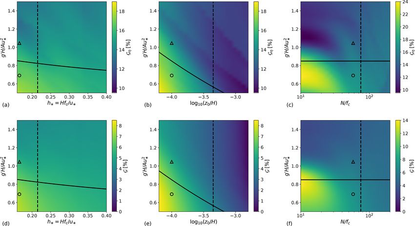
250                       L. Lanzilao and J. Meyers: Set-point optimization in wind farms to mitigate effects of flow blockage

f (1) = −βCT B(x, y)U0 · u1 ,                                    (6)    plex stratification coefficient 8̂ in Fourier components is ex-
                                                                        pressed as
where
                                                                                     i N 2 − 2

      1
                                                                        8̂ = g 0 +                .                               (10)
  0
U =        U 1 ⊗ U 1 + IkU 1 k2                                  (7)                      m
    k U1 k
and with B(x, y) a box function equal to 1 within the wind-             Relation (Eq. 10) is obtained from linear three-dimensional,
farm area and zero outside. The x and y axes denote the                 non-rotating, non-hydrostatic gravity-wave theory (Nappo,
streamwise and spanwise directions, respectively. The wind-             2002) under the assumption of constant wind speed U g =
farm drag force magnitude in Eqs. (5) and (6) scales with               (Ug , Vg ) and Brunt–Väisälä frequency N. The reduced grav-
                                                                        ity g 0 = g1θ/θ0 accounts for two-dimensional trapped lee
      π ηw γ                                                            waves (from here on named inversion waves) which corru-
β=           ,                                                   (8)
      8sx sy                                                            gate the capping inversion layer. The potential-temperature
                                                                        difference 1θ denotes the strength of the capping inversion,
where sx and sy are the streamwise and spanwise turbine                 and θ0 is a reference potential temperature. The effect of in-
spacings relative to the rotor diameter, ηw is the wake                 ternal gravity waves is represented by the second term of re-
efficiency and γ = u2r / k U 1 k2 is a velocity shape factor            lation (Eq. 10), where m denotes the vertical wavenumber
with ur the rotor-averaged wind speed (Allaerts and Mey-                which is given by
ers, 2018). Moreover, I = ex ⊗ ex + ey ⊗ ey denotes the unit
dyadic. Finally, CT (x, y, t) represents the thrust-coefficient                   N2
                                                                          2  2   2
distribution. To compute the thrust coefficient C       eT,k (t) of a   m = k +l        −1 .                                      (11)
                                                                                     2
turbine at location (xk , yk ), it is possible to evaluate the thrust
set-point distribution CT (xk , yk , t). A more accurate connec-        According to the sign of m2 , we can have propagating
tion between C eT,k (t) and the drag force f would, for exam-
                                                                        or evanescent waves. Moreover,  = ω − κ · U g denotes
ple require the use of an analytical wind-farm wake model.              the intrinsic wave frequency with κ = (k, l) the horizontal
This is however not considered in the current work, so that             wavenumber vector.
wake effects are not explicitly incorporated in the optimiza-              Finally, combining Eq. (9) with Eqs. (2) and (4), we can
tion. Rather, we consider the optimization of the gravity-              write the continuity equations for the wind farm and upper
wave system, while presuming that the wake efficiency pa-               layer as
rameter ηw does not change as a result of the optimization.
Relation (Eq. 6) is nonlinear since it contains a product be-           1 ∂p1  1                  h            i
tween time- and space-dependent variables (i.e. CT and u1 ).                  + U 1 · ∇p1 + H1 ∇ · F −1 (8̂)∗u1 = 0,              (12)
                                                                        ρ0 ∂t  ρ0
We decide to retain this term because it allows us to include           1 ∂p2  1                  h            i
gravity-wave feedback on wind-farm energy extraction. In                      + U 2 · ∇p2 + H2 ∇ · F −1 (8̂)∗u2 = 0,              (13)
fact, f (1) ≥ 0 so that it reduces the drag force that the farm         ρ0 ∂t  ρ0
exerts on the flow, thereby reducing effects of blockage in             where p = p1 +p2 is intended as the sum of the pressure per-
the model. We note that Allaerts and Meyers (2019) have                 turbations induced by the vertical displacements η1 and η2 ,
shown that the flow perturbations computed with this simple             respectively. This form will be used in the remainder of the
drag force model have similar trends and orders of magnitude            manuscript.
as the ones computed using a drag model that relies on the
more detailed analytical wake model of Niayifar and Porté-
Agel (2016). Therefore, we believe that the model adopted is            2.2   Optimization model
a reasonable representation of reality.
                                                                        The goal of the optimization framework is to find a time-
   The total vertical displacement of the inversion layer ηt =
                                                                        periodic optimal thrust-coefficient distribution CTO (x, y, t)
η1 + η2 triggers gravity waves which induce pressure pertur-
                                                                        that minimizes the gravity-wave-induced blockage effects,
bations p. The relation between these two quantities is given
                                                                        maximizing the flow wind speed and consequently the wind-
by Smith (2010):
                                                                        farm energy extraction over a selected time period T . The
p                                                                       background atmospheric state is presumed to be steady,
   = F −1 (8̂)∗ηt ,                                              (9)    which is the reason why we use a time-periodic control
ρ0
                                                                        (i.e. leading to a moving time average of the optimal con-
where F −1 and ∗ denote the inverse Fourier transform and               trol that is steady and does not lead to end-of-time effects).
the convolution product, respectively. The pressure p is eval-          The wind-farm layout and the atmospheric state are inputs
uated at the capping inversion height, and it is assumed                of the optimization model and are detailed in Sect. 3. Note
to be constant through the whole ABL (using the clas-                   that the relation between overall wind-farm drag and wind-
sical boundary-layer approximation ∂p/∂z = 0). The com-                 farm blockage is non-trivial. On the one hand, increased

Wind Energ. Sci., 6, 247–271, 2021                                                            https://doi.org/10.5194/wes-6-247-2021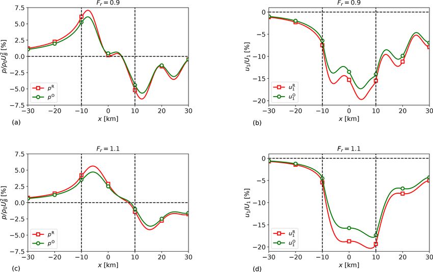
L. Lanzilao and J. Meyers: Set-point optimization in wind farms to mitigate effects of flow blockage                            251

wind-farm drag leads to increased wind-farm blockage in-
duced by gravity waves. This results from mass conserva-          minψ,CT J (ψ, CT )
tion and the upward displacement of the free atmosphere. On                s.t.
the other hand, increased wind-farm blockage reduces wind-
                                                                           ∂u1                      1          1
farm drag. Thus, the aim of the optimization is to find the                      + U 1 · ∇u1 + ∇p1 + ∇p2 + fc J
optimal balance between these two opposing trends.                          ∂t                     ρ0          ρ0
                                                                                                   D 0                C0
   By using axial momentum theory (Burton et al., 2001),
                                                                           · u1 − νt,1 ∇ 2 u1 −        · (u2 − u1 ) +    · u1
we find that the power coefficient Cp (x, y, t) depends upon                                      H1                  H1
the thrust coefficient according to the following non-linear                    f (0) + f (1)
relationship:                                                               =                  in  × (0, T ],
                                                                                     H1
       CT     p                                                          ∂u2                      1          1
Cp =        1 + 1 − CT .                                  (14)                   + U 2 · ∇u2 + ∇p1 + ∇p2 + fc J
        2                                                                   ∂t                     ρ0          ρ0
                                                                                                   D 0
The objective function of the optimization model consists in               · u2 − νt,2 ∇ 2 u2 +
the energy extracted by the farm in the time interval [0, T ];                                    H2
hence it is defined as                                                     · (u2 − u1 ) = 0 in  × (0, T ],
                                                                            1 ∂p1        1
                           ZT ZZ                                                      + U 1 · ∇p1 + H1 ∇
                                                                           ρ0 ∂t        ρ0
J (ψ, CT ) = − β k U 1 k           Cp B(x, y)                                h                i
                                                                                 −1
                                                                           · F (8̂)∗u1 = 0 in  × (0, T ],
                           0
                                                                            1 ∂p2     1

                      2
                 kU 1 k + 3U 1 · u1 dxdt,                 (15)                     + U 2 · ∇p2 + H2 ∇
                                                                           ρ0 ∂t      ρ0
                                                                             h           i
where  = Dx × Dy is the computational domain area. The                    · F −1 (8̂)∗u2 = 0 in  × (0, T ],
non-linear relationship between Cp and CT and the product
between control and state variables in Eq. (15) imply that the             0 ≤ CT < 1 in  × (0, T ],
objective function J is non-convex.                                        CT (x, y, 0) = CT (x, y, T ) in .                   (16)
   The wind-farm optimal configuration that maximizes the
energy output (note that the objective function is defined with   The constraints are the state (or forward) equations presented
a minus sign) is then obtained by solving the following non-      in the previous paragraph. Since Eq. (14) is defined only for
linear time-periodic optimization problem constrained by a        CT ∈ [0, 1), we added a box constraint to the optimization
system of partial differential equations (PDEs):                  model. Moreover, the time periodicity is imposed by assum-
                                                                  ing CT (x, y, 0) = CT (x, y, T ). The system state ψ = [u1 ,
                                                                  v1 , u2 , v2 , p1 , p2 ] includes the velocity and pressure pertur-
                                                                  bations in the wind farm and upper layer, which also define
                                                                  the unknowns of the three-layer model. The control param-
                                                                  eters consist of the value of the thrust set point in each grid
                                                                  cell within the wind-farm area. Hence, the size of the con-
                                                                  trol space is proportional to Nxwf Nywf Nt , where Nt represents
                                                                  the number of time steps within the time horizon T , while
                                                                  Nxwf and Nywf denote the number of grid points within the
                                                                  wind-farm area along the x and y directions, respectively.
                                                                     It is common practice in a PDE-constrained optimization
                                                                  problem to not optimize the cost functional J (ψ, CT ) di-
                                                                  rectly because such a problem would span both the state and
                                                                  control space. To avoid exploring the entire feasibility region,
                                                                  we require ψ(CT ) to be the solution of the state equations
                                                                  throughout the optimization process. In other words, defin-
                                                                  ing an operator N (ψ, CT ) that denotes the state equations,
                                                                  we are enforcing N (ψ(CT ), CT ) = 0 during optimization it-
                                                                  erations. This technique leads us to a reduced optimization
                                                                  problem with feasibility region given by the control space
                                                                  (De Los Reyes, 2015). The reduced optimization problem is
                                                                  written as

https://doi.org/10.5194/wes-6-247-2021                                                     Wind Energ. Sci., 6, 247–271, 2021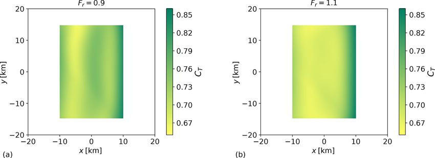
252                       L. Lanzilao and J. Meyers: Set-point optimization in wind farms to mitigate effects of flow blockage

                                                                      roughly the same as for the forward equation, the computa-
minCT Je(CT ) = J (ψ (CT ) , CT )                                     tional cost for evaluating ∇ Je is proportional to the cost of
                                                                      solving twice the state equations. To verify the approach, we
               s.t.
                                                                      compare the adjoint gradient to a standard finite-difference
               0 ≤ CT < 1 in  × (0, T ],                             approximation in Appendix A4.
               CT (x, y, 0) = CT (x, y, T ) in ,              (17)

where the only remaining constraints are the ones on the con-         3     Numerical setup and case description
trol parameters.
                                                                      We define the model setup used to assess the potential of set-
   The gradient of the reduced objective function ∇ Je is
                                                                      point optimization in mitigating self-induced gravity-wave
needed for the solution of the reduced optimization problem.
                                                                      effects in this section. We discuss the numerical setup in
To this end, we use the continuous adjoint method. The ad-
                                                                      Sect. 3.1. Next, the selected wind-farm layout is presented
joint (or backward) equations are given by (see Appendix A2
                                                                      in Sect. 3.2. Finally, the atmospheric state is discussed in
for detailed derivation)
                                                                      Sect. 3.3.
    ∂ζ 1                                            D0
−        − U 1 · ∇ζ 1 + fc J · ζ 1 − νt,1 ∇ 2 ζ 1 +    ·ζ
     ∂t                                             H1 1              3.1    Numerical setup
            C0         D0              h
                                                                      Both the forward and adjoint equations are discretized using
         +      ·ζ1 −      · ζ 2 − H1 F −1 (8̂)(−x, −t)
           H1          H2                                             a Fourier–Galerkin spectral method in space and time. The
                    βCT B(x, y) 0                                     use of Fourier modes in time automatically results in sat-
         ∗∇51 ] +                  U · ζ 1 = 3βCp B(x, y)
                         H1                                           isfying the periodicity conditions that we are aiming for in
         k U 1 k U 1 in  × (0, T ],                                  our optimization setup. All terms in the equations are linear,
                                                                      except for the first-order term of the wind-farm drag force
          ∂ζ 2                                            D0
        −      − U 2 · ∇ζ 2 + fc J · ζ 2 − νt,2 ∇ 2 ζ 2 +             (and its adjoint). These terms contain products between tem-
           ∂t                                             H2          porarily and spatially dependent variables. To avoid expen-
               D 0           h                             i
        ·ζ2 −      · ζ 1 − H2 F −1 (8̂)(−x, −t)∗∇52                   sive convolution sums, these products are computed in phys-
               H1                                                     ical space. Full dealiasing is obtained by padding and trunca-
        = 0 in  × (0, T ],                                           tion according to the 3/2 rule (Canuto et al., 1988). The use
          ∂51                                                         of Fourier modes in space forces periodic boundary condi-
        −       − U 1 · ∇51 − ∇ · ζ 1 − ∇ · ζ 2                       tions at the edges of the computational domain. Therefore,
            ∂t
                                                                      the domain has a sufficiently large dimension Dx × Dy =
        = 0 in  × (0, T ],
                                                                      1000×400 km2 , so that the perturbations die out before being
          ∂52                                                         recycled. The grid has Nx × Ny = 4000 × 1600 grid points,
        −       − U 2 · ∇52 − ∇ · ζ 1 − ∇ · ζ 2
            ∂t                                                        which corresponds to a space resolution of 1 = 250 m or
        = 0 in  × (0, T ].                                    (18)   6.4 × 10⁶ DOF per layer. Finally, different time horizon val-
                                                                      ues are used spanning from T = 10 min to T = 10 h with the
Note that the minus sign in the argument of F −1 (8̂)(−x, −t)         number of time steps ranging from Nt = 12 to Nt = 120.
is not a result of classical integration by parts, but rather ar-     The discretized forward and backward equations form two
rives from applying Fubini’s theorem to the convolution term          systems of the dimension 6Nx Ny Nt × 6Nx Ny Nt , which are
in Eqs. (12) and (13) (see Appendix A2 for details). The ad-          solved using the LGMRES algorithm (Baker et al., 2005).
joint variables are grouped in the vector ψ ∗ = [ζ 1 , ζ 2 , 51 ,        For the optimization, two different algorithms are com-
52 ], where ζ 1 = (ζ1 , χ1 ) and ζ 2 = (ζ2 , χ2 ) are the adjoint     pared in Fig. 1. The L-BFGS-B (limited-memory Broyden–
velocity perturbation fields in the wind farm and upper layer,        Fletcher–Goldfarb–Shanno with box constraint) algorithm
respectively, while 51 and 52 are the adjoint pressure pertur-        (Byrd et al., 1995) is an iterative quasi-Newton method. In
bations. Using the solution of the adjoint equations, the gra-        the current application, the step length is evaluated with the
dient of the cost function is expressed as (see Appendix A3           inexact line search Wolfe condition (Wolfe, 1969). The trun-
for details)                                                          cated Newton method (TNC) computes the search direction
        βB(x, y)

                                                dCp                   by solving the Newton equation iteratively, applying the con-
∇ Je =              kU 1 kU 1 · ζ 1 − H1 kU 1 k                       jugate gradient method. This inner loop is stopped (trun-
           H1                                   dCT
                                             i                      cated) as soon as a termination criterion is satisfied (Nocedal
                2                    >   0                            and Wright, 1999). In both cases, the system matrix of the
          kU 1 k + 3U 1 · u1 + u1 · U · ζ 1 ,                (19)
                                                                      Newton equation consists of an approximate Hessian ma-
where dCp /dCT is computed from Eq. (14). To compute the              trix, while the right-hand side needs gradient information to
gradient ∇ Je, we need to solve the forward and backward              be computed, which is provided by the continuous adjoint
equations. Since the cost for solving the adjoint equations is        method (see Appendix A for derivation and validation). Fig-

Wind Energ. Sci., 6, 247–271, 2021                                                       https://doi.org/10.5194/wes-6-247-2021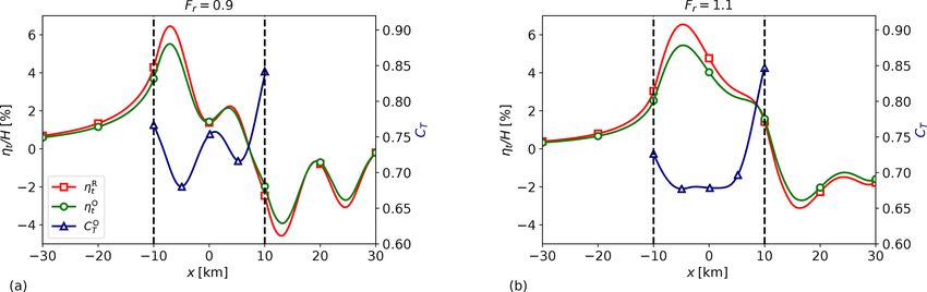
L. Lanzilao and J. Meyers: Set-point optimization in wind farms to mitigate effects of flow blockage                                 253

Figure 1. Convergence of the cost functional over the (a) L-BFGS-B and (b) TNC iteration. The squares and triangles denote the cost
functional value and the number of function evaluations, respectively.

ure 1 shows that the cost function decreases rapidly in the              ically increase with the size of the farm. Also, they men-
first two to three algorithm iterations, reaching a plateau af-          tion that the losses are at a maximum when the wind-farm
terwards. The use of a quasi-Newton method in combination                ratio Ly /Lx is close to 3/2, while being negligible for a
with the limited complexity of our optimization model (for               very wide but short farm, and vice versa (i.e. negligible for
instance, the constraints are linearized equations) allow us to          Ly /Lx  1 and Lx /Ly  1). Since we are interested in op-
reach such a fast convergence. Moreover, the continuous ad-              timal thrust-coefficient distributions in the presence of grav-
joint method limits the number of function evaluations, since            ity waves, we have selected the “worst-case” wind-farm lay-
it is not necessary to evaluate Je(CT + αδCT ) for all direc-            out (i.e. a wind-farm width and length of Ly = 30 km and
tions δCT in the control space (at the expense of solving an             Lx = 20 km, respectively). We note that this was also the
auxiliary set of equations). In particular, Fig. 1a shows that           farm layout chosen by Allaerts et al. (2018) and Allaerts and
the cost functional is converged after six L-BFGS-B itera-               Meyers (2019), which in size resembles the Belgian–Dutch
tions. Apart from the first iteration, the line search method            wind-farm offshore cluster located in the North Sea, but
needs three “function evaluations” before updating the cost              simplified to a rectangular-shaped wind farm. Also, Smith
functional. Hence, we need to solve 20 times the forward and             (2010), Fitch et al. (2012) and Wu and Porté-Agel (2017)
backward equations for reaching convergence. On the other                have used a farm with similar dimensions in their studies.
hand, Fig. 1b illustrates that the cost functional is mainly             The wind turbine relative spacings along the x and y direc-
minimized within the first TNC iteration, and convergence is             tions are sx = sy = 5.61 (both non-dimensionalized with re-
reached after only four iterations. However, 63 function eval-           spect to the turbine rotor diameter D), so that the density of
uations are needed. Hence, we will use the L-BFGS-B algo-                turbines in the farm is similar to the one of Allaerts and Mey-
rithm for solving the PDE-constrained optimization problem               ers (2019) (i.e. leading to β = 0.01 in Eq. (8), setting both the
in the remainder of the article. To limit computational effort,          wake efficiency ηw and γ to 0.9 as in Allaerts and Meyers,
a maximum of four L-BFGS-B iterations will be performed.                 2018). Note that we do not define a specific layout or a num-
   The solver (which is not parallelized) takes a couple                 ber of turbines, but we only fix the density of turbines in the
of hours to solve the equations for a grid with resolution               farm. The turbine dimensions are based on a DTU 10 MW
of 250 m (6.4 × 10⁶ DOF per layer). Since convergence is                 IEA wind turbine (Bortolotti et al., 2019) with rotor diame-
reached after approximately 20 function evaluations (which               ter D = 198 m and turbine hub height zh = 119 m.
means that we solve state and adjoint equations 20 times),
the optimizer takes a couple of days to compute an optimal               3.3   Background state variables
thrust set-point distribution. However, after this work was
performed, we have upgraded the forward solver which is                  The governing equations are linearized around a constant
now approximately 1000 times faster than our previous ver-               background state. To determine this state, we need vertical
sion. Optimization of the backward solver is planned for the             profiles of potential temperature, velocity, shear stress and
future, and we expect that this will lead to an optimization             eddy viscosity plus the surface roughness z0 and the friction
algorithm that will only take several minutes for the same               velocity u∗ . We describe the techniques used in determining
case.                                                                    these profiles in the remainder of this section. Similar to Al-
                                                                         laerts and Meyers (2019), we select two atmospheric states
                                                                         for initial testing of the optimizer, corresponding to sub- and
3.2   Wind-farm layout
                                                                         supercritical flow conditions.
Allaerts and Meyers (2019) conducted a sensitivity study                    We choose a temperature profile that corresponds to a con-
on the effects of wind-farm layout on gravity-wave-induced               ventionally neutral ABL. The potential temperature in the
power losses. They show that these power losses monoton-                 neutral ABL is fixed to θ0 = 288.15 K. A capping inversion

https://doi.org/10.5194/wes-6-247-2021                                                           Wind Energ. Sci., 6, 247–271, 2021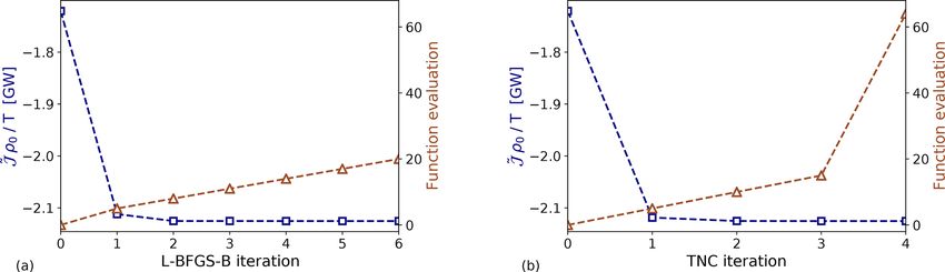
254                     L. Lanzilao and J. Meyers: Set-point optimization in wind farms to mitigate effects of flow blockage

strength 1θ of 5.54 and 3.7 K is used, which leads to a            Table 1. Numerical setup, wind-farm layout and atmospheric state
sub- and supercritical flow, respectively (see below). Finally,    used in this manuscript.
a free-atmosphere lapse rate 0 = 1 K km−1 is chosen. The
lapse rate also defines the Brunt–Väisälä frequency N .             Numerical setup
   The velocity and stress profiles within the ABL are ob-          Domain size                  Dx × Dy = 1000 × 400 km2
tained following the approach of Nieuwstadt (1983). The             Grid size                    Nx × Ny = 4000 × 1600
non-dimensional surface roughness length z0 = z0 /H and             Grid resolution              1 = 250 m
the non-dimensional boundary-layer height h∗ = H fc /u∗             Time horizon                 Span from T = 10 min to T = 10 h
are the input parameters of Nieuwstadt model, where fc is the       Time step                    Span from Nt = 12 to Nt = 120
Coriolis frequency and H = H1 + H2 is the ABL height. The           Discretization technique     Fourier–Galerkin
wind-farm layer height is assumed to be twice the turbine           Equation solver              LGMRES
                                                                    Optimization method          L-BFGS-B
hub height, so H1 = 2zh . The ABL height is fixed to H =            L-BFGS-B iterations          Nit = 4
1000 m and the friction velocity is set to u∗ = 0.6 m s−1 . Fi-
nally, a surface roughness of z0 = 10−1 m is adopted. Using         Wind-farm layout
h∗ = 0.166 and z0 = 10−4 as input values for the Nieuw-             Wind-farm length             Lx = 20 km
stadt model, we derive the velocity U 1 , U 2 , the eddy vis-       Wind-farm width              Ly = 30 km
cosity νt,1 , νt,2 for the wind-farm and upper layer, and the       Turbine hub height           zh = 119 m
friction coefficients C and D (used for computing the matri-        Turbine rotor diameter       D = 198 m
ces C0 and D0 ; see Allaerts and Meyers, 2019). Besides the         Rated wind speed             Ur = 11 m s−1
friction coefficients C and D, which are given at z = 0 and         Relative turbine spacing     sx = sy = 5.61
                                                                    Wake efficiency              ηw = 0.9
z = H1 , all other physical quantities are depth-averaged over
                                                                    Velocity shape factor        γ = 0.9
the height H1 and H2 . Finally, the wind profile is oriented
such that the wind in the wind-farm layer is always directed        Atmospheric state
along the x axis (i.e. V1 = 0 m s−1 ).                              ABL potential temperature    θ0 = 288.15 K
   The pressure gradient strengths induced by inversion and         Capping inversion strength   1θ = 5.54 K → F r = 0.9
internal gravitypwaves are dependent upon the Froude num-                                        1θ = 3.70 K → F r = 1.1
ber F r = UB / g 0 H and a non-dimensional group PN =               Free-atmosphere lapse rate   0 = 1 K km−1
UB2 /N H k U g k, respectively (Smith, 2010; Allaerts and           Surface roughness            z0 = 10−1 m
Meyers, 2019), where the velocity scale UB is defined as            Coriolis frequency           fc = 10−4 s−1
                                                                    Friction velocity            u∗ = 0.6 m s−1
                          !1                                        Boundary layer height        H = 1000 m
                             2
         H1 1    H2 1
UB =           +                 .                         (20)     Friction coefficients        C = 3.76 × 10⁻³
         H U12   H U22                                                                           D = 1.51 × 10⁻¹

The chosen background state defines a Froude number of 0.9
for 1θ = 5.54 K, which implies subcritical flow conditions
(F r < 1), and a Froude number of 1.1 for 1θ = 3.7 K,              time-periodic optimal thrust-coefficient distribution over the
which leads to supercritical flow conditions (F r > 1). Fur-       wind-farm area in a fixed time interval [0, T ]. However, all
ther, PN expresses the impact of internal waves in the tropo-      optimal thrust set-point distributions found for the different
sphere, which increases when PN decreases. The background          combinations of time horizons and time steps reported in Ta-
state defined in Table 1 leads to PN = 1.92. The numerical         ble 1 are constant in time. We have verified this using a range
setup, wind-farm layout and background state variables are         of steady and unsteady starting conditions for CT in the al-
summarized in Table 1.                                             gorithm, but we did not find any unsteady optimum. We be-
                                                                   lieve that this is due to the use of steady-state inflow con-
4     Results and discussion                                       ditions, meaning that we neglect meso-scale temporal varia-
                                                                   tions in the velocity field (these could lead to time-dependent
We discuss the results of the optimization problem in the cur-     optimal control signals, but are not included in the current
rent section. Firstly, the optimal thrust-coefficient distribu-    work). Since we do not observe any unsteady behaviour in
tions and relative power gains are illustrated for two specific    our optimal solutions, we show only steady-state results in
flow conditions in Sect. 4.1. Thereafter, the sensitivity of the   the remainder of the manuscript, and we conclude for the
power gain to the atmospheric state is studied in Sect. 4.2.       time being that unsteady time-periodic excitation is less ef-
                                                                   fective than a stationary spatially optimal distribution in this
                                                                   context.
4.1    Optimal thrust-coefficient distributions
                                                                      We also note that our findings are in contrast with re-
The optimization model described in Sect. 2.2 is time and          cent works of Goit and Meyers (2015), Munters and Mey-
space dependent. Hence, the model is capable of finding a          ers (2018), and Frederik et al. (2020), in which the authors

Wind Energ. Sci., 6, 247–271, 2021                                                      https://doi.org/10.5194/wes-6-247-2021
L. Lanzilao and J. Meyers: Set-point optimization in wind farms to mitigate effects of flow blockage 255
illustrated the benefits of dynamic induction control over deficits within the wind-farm area. This explains the higher
yaw and static induction control. However, the characteristic velocity reduction (up to 20 %) seen in Fig. 2f. Such a strong
timescale of gravity-wave effects is estimated to be approxi- response could be on the limit of our small amplitude as-
mately 1 h (Gill, 1982; Allaerts and Meyers, 2019), which is sumption. The planform view of pressure and velocity per-
an order of magnitude above the typical timescale of wake turbations in the wind-farm and upper layer in subcritical
convection between turbines, and turbulent mixing in tur- flow conditions are also illustrated on a wider domain in Ap-
bine wakes (this also justifies the larger sampling time used). pendix A (see Fig. A1).
Hence, while unsteadiness of the thrust coefficient (with a The goal of our study is to find an optimal set-point distri-
typical timescale of 50 s for large-scale turbines) can lead bution which reduces the velocity perturbations displayed in
to improved wake mixing (Goit and Meyers, 2015; Munters Fig. 2c and f. While maximizing the flow wind speed through
and Meyers, 2018; Frederik et al., 2020), it has no impact the farm, we also maximize the wind-farm energy extraction.
on phenomena that occur at larger timescales, such as wind- To this end, we solve the optimization problem discussed in
farm-induced gravity waves. Sect. 2.2. The inputs of the optimization model are the wind-
The steady-state optimal thrust-coefficient distributions farm layout and the atmospheric conditions, which are de-
obtained in sub- and supercritical conditions are analysed in tailed in Table 1. Moreover, an initial thrust-coefficient distri-
the remainder of this section. To improve the understanding bution needs to be specified. We have verified that for many
of such distributions, gravity-wave-induced flow patterns ob- different initial conditions the algorithm always converges
tained with CTO (x, y) are compared with a reference case. to the same optimal solution. Therefore, a random initial
The setup of the reference model is the one reported in Ta- thrust set-point distribution is chosen. The optimal configu-
ble 1, but instead a uniform thrust set-point distribution over rations obtained for different Froude numbers are illustrated
the wind-farm area is used, with CTR (x, y) = CTBetz = 8/9. in Fig. 3. We find that the optimal thrust-coefficient distribu-
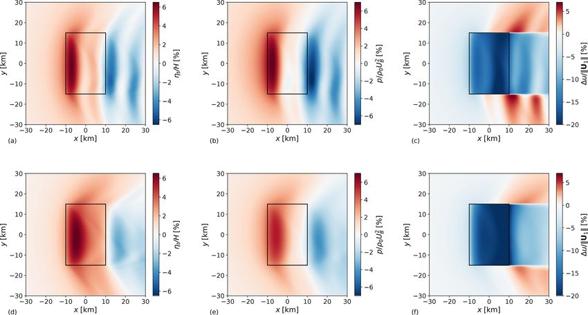
Figure 2 illustrates a planform view of the perturbation tions are non-uniform in space and assume different spatial
flow patterns obtained with F r = 0.9 (top row) and F r = 1.1 distributions according to the atmospheric state. In particular,
(bottom row) using the reference model setup. The farm ex- when the flow is subcritical the optimal thrust set-point dis-
tracts energy from the flow, causing a momentum sink in tribution assumes a sinusoidal behaviour in the streamwise
the wind-farm layer. Due to the continuity constraint, an direction while it becomes a U-shaped curve when the flow
upward flow displacement above the wind-farm area takes is supercritical. In both cases, CTO is almost invariant along
place, which causes the boundary layer height to increase. the spanwise direction.
Figure 2a shows that an inversion-layer vertical displacement We denote with P R = J g R /T and P O = J eO /T the power
of about 65 m takes place at the wind-farm entrance region extracted using CT = CTR = 8/9 and CT = CTO , respectively.
for the subcritical case. A second peak of lower magnitude is Further, we define
located in the downwind region. On the other hand, for the
PO − PR
supercritical case, Fig. 2d displays a similar maximum value G= , (21)
of ηt attained close to the wind-farm centre. In both cases, the PR
inversion-layer vertical displacement decreases in the wind- where G denotes the relative power gain obtained using an
farm exit region and assumes a wavy behaviour in the wind- optimal thrust-coefficient distribution instead of the refer-
farm wake. The vertical displacement of air parcels triggers ence one. Note that the optimal distributions are steady state;
inversion waves on the 2D inversion-layer surface and inter- therefore the power gain definition is not dependent on the
nal waves in the free atmosphere (3D waves). These waves choice of the time horizon T . The power gains attained in
induce pressure gradients, as visible in Fig. 2b and e, where sub- and supercritical flow conditions are 5.3 % and 7 %, re-
a region of high pressure builds up in correspondence with spectively. Clearly, power gains are also strongly dependent
high ηt values, leading to flow blockage. However, Fig. 2b on the atmospheric conditions. Therefore, a sensitivity study
shows a stronger adverse pressure gradient in the wind-farm is carried out in Sect. 4.2. To assess the benefit of an opti-
induction region than the one in Fig. 2e. In fact, inversion mal non-uniform distribution over an optimal uniform one,
waves travel upstream in subcritical conditions, which leads we have applied the optimization framework developed in
to more slow-down in the induction region. In both the sub- Sect. 2.2 assuming a spatially invariant CT . Results are dis-
and supercritical cases, favourable pressure gradients reduce cussed in Appendix B.
the velocity deficits in the bulk of the farm. Finally, Fig. 2c The optimal set-point distributions displayed in Fig. 3 are
and f illustrate relative velocity reductions in the wind-farm related to the vertical displacement of the inversion layer
layer. The stronger inversion strength found in the subcriti- over the wind-farm area. Figure 4 shows streamwise profiles
cal flow case transforms the inversion layer in a quasi-rigid of ηt and CTO through the centre of the farm for F r = 0.9 and
lid, which limits vertical displacements. The lower stream- F r = 1.1. To reduce gravity-wave excitation, CTO is seen to
lines’ divergence over the wind-farm area implies lower ve- be inversely related with ηt . In fact, Fig. 4a shows that the
locity reductions. Moreover, the favourable pressure gradi- streamwise profile of ηt has a sinusoidal behaviour. Hence,
ent is stronger when F r = 0.9, allowing for lower velocity the optimal set-point distribution is sinusoidal as well, ex-
https://doi.org/10.5194/wes-6-247-2021 Wind Energ. Sci., 6, 247–271, 2021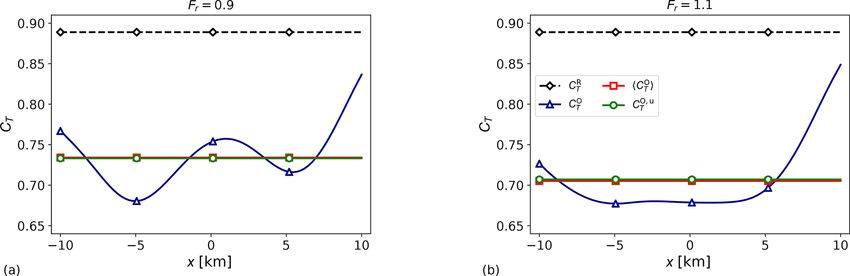
256                       L. Lanzilao and J. Meyers: Set-point optimization in wind farms to mitigate effects of flow blockage

Figure 2. Planform view of inversion-layer displacement (a, d), pressure perturbation (b, e) and relative velocity reduction (c, f) in the wind-
farm layer in subcritical (a–c, F r = 0.9) and supercritical (d–f, F r = 1.1) flow conditions. The black rectangle indicates the wind-farm
region.

Figure 3. Planform view of (a) optimal thrust-coefficient distribution in subcritical (F r = 0.9) and (b) supercritical flow conditions (F r =
1.1). The length and width of the wind farm are 20 and 30 km, respectively.

plaining the pattern displayed in Fig. 3a. On the other hand,             tion of 14.5 % and 16.8 % is attained with the optimal con-
ηt assumes a U-shaped profile through the wind farm in su-                figuration for the sub- and supercritical cases, respectively.
percritical conditions (see Fig. 4b), a profile that is also found           A lower vertical displacement of the inversion layer re-
in CTO (see Fig. 3b). Moreover, Fig. 2a and d show that the               duces gravity-wave excitation; therefore we also expect a
gradient of ηt along the spanwise direction is much smaller               lower strength of the adverse pressure gradient at the en-
than the one along the streamwise direction, explaining the               trance of the farm compared to the one obtained with CTR .
almost constant thrust set-point distributions along the y di-            Figure 5a and c confirm this hypothesis, showing stream-
                                     O
rection. Figure 4 also shows that ηt,max       R
                                           < ηt,max   in both sub-        wise profiles of pressure perturbations p R and p O through
and supercritical conditions, meaning that the optimal thrust             the centre of the farm for F r = 0.9 and F r = 1.1. The pres-
set-point distribution decreases the upward flow displace-                sure peak is located at the entrance of the farm and a pressure
ment over the wind-farm area. The maximum inversion-layer                 peak reduction of 14.3 % and 16.2 % is attained with the opti-
displacement is located at the entrance region of the farm. If            mal configuration for the sub- and supercritical cases, respec-
we compare ηtR and ηtO in this region, a displacement reduc-              tively. Figure 5b and d show streamwise profiles of velocity
                                                                          perturbations uR         O
                                                                                           1 and u1 through the centre of the farm for

Wind Energ. Sci., 6, 247–271, 2021                                                              https://doi.org/10.5194/wes-6-247-2021
L. Lanzilao and J. Meyers: Set-point optimization in wind farms to mitigate effects of flow blockage 257
Figure 4. Streamwise profiles of optimal thrust set-point distribution (CTO ), reference (ηtR ) and optimal (ηtO ) inversion-layer displacement
in (a) subcritical (F r = 0.9), and (b) supercritical flow conditions (F r = 1.1). The wind-farm region is marked by vertical dashed lines, and
the profiles have been obtained through the centre of the farm (y = 0).
Figure 5. Streamwise profiles of (a, c) reference (p R ) and optimal (p O ) pressure perturbation and (b, d) reference (uR O
1 ) and optimal (u1 )
velocity perturbation in subcritical (a, b, F r = 0.9) and supercritical (c, d, F r = 1.1) flow conditions. The wind-farm region is marked by
vertical dashed lines, and the profiles have been obtained through the centre of the farm (y = 0).
F r = 0.9 and F r = 1.1. The lower adverse pressure gradient Table 2. Relative change in percentage between optimal and refer-
strength attained with the optimal configuration allows for a ence maximum flow perturbation values. Power gains are also in-
lower velocity perturbation u1 in the induction region with cluded.
respect to the reference case. Moreover, the optimal configu-
F r = 0.9 F r = 1.1
ration also reduces the streamline divergence, accounting for
higher flow wind speeds through the farm. Consequently, a Maximum inversion-layer displacement −14.5 % −16.8 %
velocity perturbation reduction of 13.4 % and 15.5 % is at- Maximum pressure perturbation −14.3 % −16.2 %
tained for the sub- and supercritical cases, which explains Maximum velocity perturbation −13.4 % −15.5 %
the higher power gain obtained for F r = 1.1. The relative Power gain 5.3 % 7.0 %
change in percentage between optimal and reference maxi-
mum flow perturbation values is summarized in Table 2.
The optimal thrust-coefficient distributions and power
gains discussed in this section are obtained with data listed in
https://doi.org/10.5194/wes-6-247-2021 Wind Energ. Sci., 6, 247–271, 2021258 L. Lanzilao and J. Meyers: Set-point optimization in wind farms to mitigate effects of flow blockage
Table 1. However, the atmospheric state changes in real case choice of the four ranges for the non-dimensional groups dis-
scenarios, and we have seen that the optimal configuration cussed above ensures that U1 /Ur ≤ 0.9 for all atmospheric
strongly depends upon the atmospheric parameters. There- states.
fore, the sensitivity of the power gain to the atmospheric state Using the atmospheric state reported in Table 1, the
is performed in the next section. non-dimensional numbers assume values h∗ = 0.166, z0 =
10−4 and N/fc = 58. The inversion parameter is equal
4.2 Sensitivity study
to 1.046 and 0.691 in the sub- and supercritical cases, respec-
tively. The optimal thrust-coefficient distributions discussed
Allaerts and Meyers (2019) pointed out that gravity-wave- in Sect. 4.1 were obtained using these dimensionless group
induced power loss is significant only for certain atmospheric values. The sensitivity of the power gain to atmospheric con-
states. Since our aim is to recover its power loss, we also ex- ditions is performed by varying h∗ , z0 and N/fc against
pect the power gain to be sensitive to the atmospheric condi- the inversion parameter g 0 H /Au2∗ , similarly to Allaerts and
tions. We note that gravity-wave patterns are also sensitive to Meyers (2019). The numerical setup is the one detailed in
the wind-farm layout. However, a sensitivity study over the Table 1. However, we use a grid cell size which is 4 times
wind-farm layout is beyond the scope of the article. bigger (1x × 1y = 1000 × 1000 m2 ), meaning that we use
The nondimensionalization of the three-layer model equa- 4 × 10⁵ cells instead of 6.4 × 10⁶ , so that the necessary com-
tions with respect to the boundary layer height H and the putational resources remain reasonable. To assess the validity
friction velocity u∗ highlights four non-dimensional groups of this choice, we performed a grid sensitivity study in Ap-
that govern the atmospheric state, which are as follows. pendix C showing that the power gain value changes about
1 % when the number of grid cells is increased by 1 order of
– The non-dimensional boundary layer height h∗ = magnitude (see Fig. C1). The high computational efficiency
H fc /u∗ . Values of h∗ ≈ 0.1 denote shallow boundary of the three-layer model allowed us to perform a sensitivity
layers typically found over sea, while h∗ ≈ 0.35 rather study of the optimization results over 1960 different atmo-
relates to a deep land-based boundary layer. We vary h∗ spheric conditions (thus effectively running an optimization
between 0.16 and 0.4. problem for every atmospheric state). Since the wind-farm
layout impact on power gains is beyond the scope of our
– The non-dimensional surface roughness length z0 = study, we impose the wind direction to be along the x axis
z0 /H . This number varies several orders of magnitude in the wind-farm layer in all simulations (V1 = 0 m s−1 ).
according to the sea state or land surface. We vary To better understand the power gain sensitivity to atmo-
log10 (z0 ) between −4.2 and −2.8 in the current study. spheric conditions, we examine how the non-dimensional
parameters F r and PN impact the flow fields. The pres-
– The non-dimensional Brunt–Väisälä frequency N/fc .
sure gradients induced by inversion waves scale with g 0 ;
The Brunt–Väisälä frequency is an important param-
therefore high inversion strengths correspond to strong
eter in gravity-wave theory which expresses the high-
inversion-wave feedback and low Froude number values.
est possible frequency for internal gravity waves (Gill,
These p two-dimensional waves are non-dispersive with phase
1982). Typical values of free-atmosphere lapse rate 0
speed g 0 H (Sutherland, 2010). Therefore, F r also repre-
range between 1 and 10 K km−1 . Low and high 0 val-
sents the ratio of the bulk wind speed within the ABL to the
ues are associated with weakly and strongly stratified
velocity of the inversion waves. If F r < 1 (subcritical flow)
atmospheres, respectively. We vary 0 between 0.03 and
the two-dimensional waves can affect the upstream flow,
12 K km−1 corresponding to 10 ≤ N/fc ≤ 200.
while they can travel only downstream if F r > 1 (supercrit-
– The inversion parameter g 0 H /Au2∗ . According to ical flow). The flow is said to be critical when F r = 1. On
Csanady (1974), the height of the inversion layer is de- the other hand, internal-wave-induced pressure gradients are
termined by a balance of surface stress and buoyancy. governed by the second non-dimensional group PN . Strong
Equilibrium conditions are reached when g 0 H /Au2∗ ≈ internal-wave feedback corresponds to low PN values. In
1, with A = 500 being an empirical constant. We vary fact, strongly stratified atmospheres imply high N values,
the inversion parameter between 0.5 and 1.5. meaning that they account for higher internal-wave oscilla-
tion frequencies and phase speed (Sutherland, 2010).
Allaerts and Meyers (2019) conducted a similar sensitivity Two different flow regimes can be identified.
study on the gravity-wave-induced power loss on a wider
range of non-dimensional numbers. However, since we are
optimizing turbine thrust set points, we need to ensure that – Regime 1 represents low-PN flows. The strongly strati-
U1 /Ur < 1 (Ur = 11 m s−1 is the rated wind speed of the fied free atmosphere limits vertical displacement of air
DTU 10 MW IEA wind turbine), otherwise turbines would parcels; hence reduced streamline divergence over the
operate in an above-rated wind speed regime and it would wind-farm area is observed. This results in low veloc-
not make any sense to optimize their power production. The ity reductions and ηt values. Moreover, the flow fields
Wind Energ. Sci., 6, 247–271, 2021 https://doi.org/10.5194/wes-6-247-2021You can also read