QUANTIFYING THE EFFECTS OF CONTACT TRACING, TESTING, AND CONTAINMENT MEASURES IN THE PRESENCE OF INFECTION HOTSPOTS - MPG.PURE
←
→
Page content transcription
If your browser does not render page correctly, please read the page content below
Quantifying the Effects of Contact Tracing, Testing, and
                                               Containment Measures in the Presence of Infection Hotspots
                                                 Lars Lorch∗ , Heiner Kremer† , William Trouleau‡ , Stratis Tsirtsis§ , Aron Szanto¶ ,
                                                                 Bernhard Schölkopf†,∗ , Manuel Gomez-Rodriguez§
                                                                                  ∗
                                                                                   ETH Zürich, llorch@student.ethz.ch
arXiv:2004.07641v5 [cs.LG] 18 May 2021

                                                        †
                                                            Max Planck Institute for Intelligent Systems, {heiner.kremer,bs}@tuebingen.mpg.de
                                                                 ‡
                                                                   École Polytechnique Fédérale de Lausanne, william.trouleau@epfl.ch
                                                             §
                                                               Max Planck Institute for Software Systems, {stsirtsis,manuelgr}@mpi-sws.org
                                                                                ¶
                                                                                  Zerobase Foundation, aron@zerobase.io

                                                                                             May 19, 2021

                                                                                                Abstract
                                                    Multiple lines of evidence strongly suggest that infection hotspots, where a single individual infects
                                                many others, play a key role in the transmission dynamics of COVID-19. However, most of the existing
                                                epidemiological models fail to capture this aspect by neither representing the sites visited by individuals
                                                explicitly nor characterizing disease transmission as a function of individual mobility patterns. In this
                                                work, we introduce a temporal point process modeling framework that specifically represents visits to the
                                                sites where individuals get in contact and infect each other. Under our model, the number of infections
                                                caused by an infectious individual naturally emerges to be overdispersed. Using an efficient sampling
                                                algorithm, we demonstrate how to apply Bayesian optimization with longitudinal case data to estimate
                                                the transmission rate of infectious individuals at the sites they visit and in their households. Simulations
                                                using fine-grained and publicly available demographic data and site locations from Bern, Switzerland
                                                showcase the flexibility of our framework. To facilitate research and analyses of other cities and regions,
                                                we release an open-source implementation of our framework.1

                                         1      Introduction
                                         As countries around the world aim to counteract rising numbers of COVID-19 infections [1], overwhelmingly
                                         growing evidence suggests that few infected people in infection hotspots, or superspreading events (SSEs),
                                         may be responsible for both explosive early growth of cases and sustained transmission in later stages [2–7].
                                         For example, in Hong Kong, the largest infection hotspots were traced back to four bars, which accounted for
                                         32.5% of all locally acquired infections from January 23 to April 28, 2020 [2]. In South Korea, an infection
                                         hotspot linked to a church was responsible for at least 60% of all recorded cases by March 18, 2020, and over
                                         1,000 infections were traced back to a single individual [8]. The first major outbreak in Germany occurred
                                         after an infected couple attended a carnival festivity in Heinsberg, with superspreading dynamics later verified
                                         by virus genome sequencing [9]. These lines of evidence suggest that, for COVID-19, the number of infections
                                         caused by single infectious individuals is overdispersed —most individuals infect few and a few infect many,
                                         exhibiting greater variance than expected under Poisson assumptions [10–12]. Using carefully annotated
                                         tracing data, this has been identified as a root cause of SSEs [2, 4–6].
                                             Most of the existing epidemiological models, including those developed and used in the context of the
                                         COVID-19 pandemic, do not explicitly represent sites of transmission, nor do they characterize exposures as
                                             1 Our   code is publicly available at: https://github.com/covid19-model/

                                                                                                     1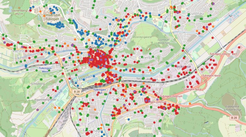
a function of individual mobility patterns. Moreover, they either assume or result in a Poisson distribution
 of infections caused by an infectious individual, also called secondary infections, which fails to capture the
 high dispersion observed for COVID-19.2 As a result, these models have been of little use for identifying
 conditions under which hotspots emerge [6, 10], helping design control measures tailored to prevent SSEs [16],
 or predicting where infection hotspots are most likely to occur [12].
     In this work, we take a first step towards addressing the above limitations and develop a flexible temporal
 point process modeling framework that explicitly represents visits to sites where exposures occur. In particular,
 we introduce
(i) an event-based “check-in” mobility model that characterizes the frequency and duration of each individual’s
    visits to specific sites, which can be configured using a variety of publicly available data, and
(ii) a new rate of transmission at sites that quantifies the influence of environmental drivers, individual mobility
     patterns, and containment measures on the risk that each infected individual poses to others at a site.
 By using this novel model of transmission and an explicit representation of the visited locations, our framework
 can directly characterize fine-grained interventions that are, for example, targeted at particular sites or
 individuals (e.g., hygienic measures at work places, closures of schools, or contact tracing). We derive an
 efficient sampling algorithm for our model, which allows us to simulate and study the spread of COVID-19
 in real-world cities and regions with hundreds of thousands of inhabitants under a variety of measures and
 what-if scenarios. Building on this procedure, we use Bayesian optimization [17–19] in combination with
 longitudinal COVID-19 case data to estimate the model parameters that control the transmission of the
 disease.
     We showcase our method using fine-grained demographic data and site locations from Bern, Switzerland,
 and other regions in Germany and Switzerland. Our results demonstrate that the number of individual
 disease transmissions—both overall and during a site visit—naturally emerges to be overdispersed, i.e.,
 exhibiting higher variance than expected under the common Poisson assumption, and that our model is able
 to robustly characterize the observed COVID-19 case trends. These findings hint at the potential of using
 our framework as a complementary policy tool for studying the efficacy of containment measures, factors of
 disease transmission, and the nature of infection hotspots—hand in hand with existing societal and ethical
 considerations. To facilitate research and analyses in this area, we release an open-source implementation of
 our framework [20].

 2      A Spatiotemporal Epidemic Model
 Given a set of individuals V, we track the current state of each single individual i ∈ V using a collection of
 state variables, which determine their mobility pattern, epidemiological condition, and testing status. The
 state transitions are modeled using stochastic differential equations (SDEs) with jumps, which faithfully
 captures (i) the stochastic nature of infection events and mobility patterns, (ii) events in continuous time, i.e.
 not in aggregate over a period, and (iii) discrete state transitions—an individual either does or does not get
 infected, visit a site, or get tested positively.
      Specifically, the jumps are modeled using temporal point processes [21]. A temporal point process is
 often represented as a counting process, say N (t), which records the number of discrete events in time
 {t1 , t2 , . . . , tn }, ti ∈ R+ before time t. The probability of an event occurring in a small time window [t, t + dt)
 is given by P (dN (t) = 1 | H(t)) = λ(t) dt with dN (t) ∈ {0, 1} and history of events H(t). The intensity
 function λ(t) can be interpreted as the instantaneous rate of events per unit of time. In what follows, to ease
 the exposition, we describe each type of state variable separately.

 2.1      Mobility
 Let S be the set of sites individuals can visit. For each individual i, let the indicator Pi,k (t) = 1 if the
 individual is at site k ∈ S at time t and Pi,k (t) = 0 otherwise. We characterize the value of the states Pi,k (t)
     2 Overdispersion   has also been observed in MERS and SARS [13–15].

                                                               2
Figure 1: Site locations by category in the mobility model of Bern, Switzerland. Circles depict
schools and research institutes (blue), social places (orange), bus stops (green), workplaces (red), supermarkets
(purple).

using the following SDE with jumps:

                                             dPi,k (t) = dUi,k (t) − dVi,k (t)                                         (1)

where Ui,k (t) and Vi,k (t) are counting processes recording the events of individual i arriving at and leaving
from site k ∈ S, respectively. We define their dynamics as follows:
                                                                    Y
                                P (dUi,k (t) = 1 | H(t)) = λi,k (t)     (1 − Pi,l (t)) dt
                                                                    l∈S                                     (2)
                                P (dVi,k (t) = 1 | H(t)) = Ui,k (t) vk dt

where λi,k (t) is the rate at which individual i visits site k and 1/vk is the average duration of a visit to site
k. To configure the rates λi,k (t) and average duration 1/vk for every individual and site, one can resort to
publicly available data. In our simulations, we use the spatial distribution of site locations, high-resolution
population density data, country-specific information about household structure, and region-specific age
demographics. We also assume that the probability that an individual i visits a specific site k decreases with
the distance between their household and the site, similar to the gravity model [22]. Figure 1 illustrates the
sites S in a mobility model of Bern, Switzerland, which will be used for the case study in Section 4.

2.2     Epidemiology
We build on recent variations of the Susceptible-Exposed-Infected-Resistant (SEIR) compartment models
that have been introduced in the context of COVID-19 modeling [23, 24]. However, while traditional SDEs
constrain the number of exposures to homogeneous Poisson distributions, we adopt a set of SDEs with jumps
that employ a stochastic and dynamically adjusting exposure rate for each individual i ∈ V, under which
this constraint is lifted. More specifically, we define the epidemiological condition of each individual i ∈ V
using the indicator state variables S(t) = {Si (t), Ei (t), Iia (t), Iip (t), Iis (t), Hi (t), Ri (t), Di (t)}i∈V with each
∈ {0, 1}, whose meaning is specified in Table 1. Their values and state transitions are characterized by the

                                                            3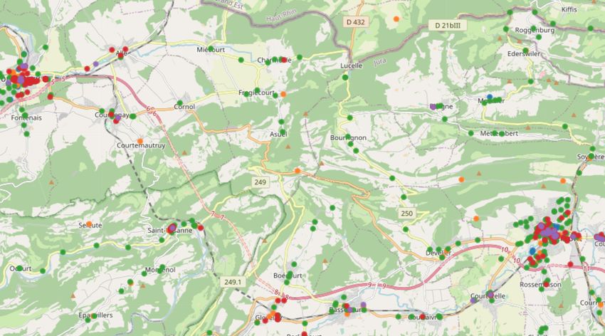
Table 1: Epidemiological state variables S(t)

                     State     Description                   Infected Contagious Symptoms
                     Si (t)    is susceptible                    -        -         -
                     Ei (t)    is exposed                        X        -         -
                     Iia (t)   is asymptomatic,
                                  mild course of disease         X        X         -
                     Iip (t)   is pre-symptomatic,
                                 progresses to Iis (t) later     X        X         -
                     Iis (t)   is symptomatic                    X        X         X
                     Hi (t)    is hospitalized                   X        X         X
                     Ri (t)    is resistant & recovered          -        -         -
                     Di (t)    has died                          -        -         -

following SDEs with jumps:
                          dSi (t) = −Si (t)dNi (t)
                          dEi (t) = dNi (t) − dMi (t)
                          dIia (t) = ai dMi (t) − dRia (t)
                          dIip (t) = (1 − ai )dMi (t) − dWi (t)
                                                                                                               (3)
                          dIis (t) = dWi (t) − (1 − bi )dRis (t) − bi dZi (t)
                          dRi (t) = ai dRia (t) + (1 − ai )dRis (t)
                         dHi (t) = hi Iis (t)dYi (t) − (1 − bi )Hi (t)dRis (t) − bi Hi (t)dZi (t)
                         dDi (t) = bi dZi (t)
where ai ∼ Bern(αa ) indicates whether an infected individual i is asymptomatic, hi ∼ Bern(αh ) whether
they eventually require hospitalization, and bi ∼ Bern(αb ) whether they eventually die.
    The counting processes C(t) = {Ni (t), Mi (t), Ria (t), Ris (t), Wi (t), Yi (t), Zi (t)}i∈V model the state
transitions. For individual i ∈ V, the first arrivals of the processes indexed by i model their transition
from susceptible to exposed (Ni (t)), from exposed to infected (Mi (t)), from presymptomatic infected to
symptomatic infected (Wi (t)), from asymptomatic infected to resistant (Ria (t)), from symptomatic infected
to resistant (Ris (t)), from symptomatic infected to hospitalized (Yi (t)), and from symptomatic infected to
dead (Zi (t)).
    At the core of our modeling framework, we define the conditional intensity function λ∗i (t) of the exposure
counting process Ni (t) as
                                       X             X Z t
                             λ∗i (t) =   βk Pi,k (t)        Kj,k (τ ) γe−γ(t−τ ) dτ                         (4)
                                      k∈S            j∈V\{i}     t−δ

where
                                   Kj,k (τ ) = Ijs (τ ) + Ijp (τ ) + µIja (τ ) Pj,k (τ )
and P (dNi (t) = 1 | H(t)) = λ∗i (t) dt. In the above:
  (i) βk ≥ 0 is the transmission rate due to presymptomatic and symptomatic individuals currently visiting
      site k. Depending on the availability of labeled and unlabeled data, one may consider sharing the same
      parameter for all sites or sites of the same category.
  (ii) µ ∈ [0, 1] is the relative transmission rate of asymptomatic compared to (pre-)symptomatic individuals.
       Rt
 (iii) t−δ Kj,k (τ ) γe−γ(t−τ ) dτ accounts for environmental transmission, i.e., it accounts for the fact that the
       virus may survive for some period of time on surfaces or in the air after an infected individual has left a
       site [25].

                                                             4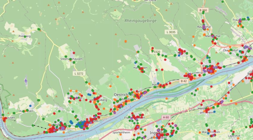
The exposure intensity in (4) models that an individual’s instantaneous rate of exposure increases by a
constant site-specific transmission rate βk when in contact with another infectious individual at a site k ∈ S,
in addition to capturing environmental transmission. Consequently, based on the mobility traces Pi,k (t), the
exposure rate of each individual i only depends on the individual’s contacts at sites k ∈ S, not the contacts
of others. Infections within households are characterized by adding an additional analogous term λH(i) (t)
with household transmission rate ξ to λ∗i (t), as outlined in Appendix A.
    For the remaining (mobility-independent) counting processes Mi (t), Ria (t), Ris (t), Wi (t), Yi (t), and
Zi (t), which characterize the state transitions after exposure, we model the times to event using log-normal
distributions [26, 27] starting at the time Ei (t), Iip (t), Iia (t) or Iis (t) become one, respectively. Their parameters
are fixed based on recent estimates by the COVID-19 literature and summarized in Table 2.

2.3     Testing
Individuals are tested according to a testing policy πtest (t), e.g., testing only symptomatic or vulnerable
people, at a rate λtest (t), which can be chosen to match location-specific testing statistics. The test outcomes
are only known after a reporting delay ∆test . Formally, the counting process T (t) records the number of
known test outcomes by time t. Let Ti+ (t) and Ti− (t) be the number of times an individual i ∈ V has been
tested positive and negative, respectively, by time t. Then, we characterize the state variables Ti+ (t) and
Ti− (t) using the following SDEs:

                             dTi+ (t) = Ei (t) + Iia (t) + Iip (t) + Iis (t) di (t) dT (t + ∆test )


                             dTi− (t) = Si (t) + Ri (t) di (t) dT (t + ∆test )

                                                                                                              (5)

where di (t) ∈ {0, 1} ∼ πtest (t) indicates whether i is tested at time t according to the policy.

2.4     Containment measures
In the above context, we can faithfully model a variety of containment measures that not only affect the
broad population V but also target specific sites or individuals, possibly in a time-variant fashion. These
may range from less restrictive (e.g., isolating individuals who have tested positive for 14 days or who had
contact with a positively tested individual) to more restrictive (e.g., implementing a state of “lockdown” for
the entire population). The effect of mobility reduction and quarantine can be characterized by reducing
the rates λi,k (t) at which individuals visit sites in the mobility model. Hygienic measures (e.g., face masks)
can be implemented by reducing the transmission rate βk at specific sites (e.g., work places). In all cases,
the measures reduce the conditional intensities λ∗i (t) of the exposure counting processes Ni (t), possibly
dynamically based on the values of other state variables at time t.
    Moreover, if desired, we may assume that contacts between individuals at sites are registered by a
peer-to-peer proximity-based tracing system, analogous to the smartphone-based Bluetooth systems that
have been implemented in the context of the COVID-19 pandemic [28]. A contact between individuals i
and j will be registered if (i) their visit times at a specific site k ∈ S overlap, and (ii) both opt to use
the proximity-based tracing system, e.g., by means of carrying a Bluetooth device. Visit times are said to
overlap when Pi,k (t) = 1 and Pj,k (t) = 1 for some k ∈ S and t. When an individual i is tested positive, their
registered contacts may be advised to isolate or seek testing themselves as described in Section 2.3. For
contact tracing, the type of intervention may depend on the risk of exposure caused by the positively tested
individual, which can be estimated using our model. Appendix B provides further details.

                                                            5
3 Model Simulation and Estimation
3.1 Epidemiological Sampling Algorithm
Having formally defined the model dynamics in Section 2, we now describe how to generate simulations
of the individual epidemiological states S(t) over a time horizon t ∈ [0, tmax ], which ultimately allows us
to empirically study the spread of the disease under a variety of scenarios. The initial conditions S(0), a
testing policy πtest (t), and the mobility traces Pi,k (t) are assumed to be fixed a priori—from simulations of a
synthetic mobility model or real-world data.
The epidemiological state variables S(t) in the model SDEs (3) change at—and only change at—events of
the counting processes C(t). Hence, all state variables S(t) are constant between two consecutive events when
considering all event times of C(t) on one timeline. This leads us to the backbone principle for generating
random realizations of the model: we initialize the state variables S(0), sample the next time of state
transition for each i ∈ V, and push these transition events onto one single temporally-sorted priority queue
Q, simultaneously tracking the next events for all individuals in the model. The algorithm then repeatedly
loops through: (i) popping the next event e from Q; (ii) updating the state of individual i associated with e;
(iii) sampling the next time t of state transition e0 for i; and (iv) pushing e0 to Q with priority t.
As explained in Section 2, we fix the time-to-event distributions of all non-exposure processes C(t)\{Ni (t)}i∈V
to independent, easy-to-sample distributions as estimated by clinical COVID-19 literature. Thus, sampling
the first event time of Ni (t) (the time of exposure of i) is the central difficulty, with rate λ∗i (t) dynamically
interacting with all other stochastic state variables S(t) via the mobility model Pi,k (t). To this end, we first
decompose the intensity λ∗i (t) into a sum of contributions λ∗j→i (t) caused by other individuals j:
X X Z t X
λ∗i (t) = βk Pi,k (t) Kj,k (τ )γe−γ(t−τ ) dτ =: λ∗j→i (t) (6)
j∈V\{i} k∈S t−δ j∈V\{i}
where the last summation over j ∈ V\{i} is sparse as it only indexes over contacts of individuals i after time
t. Note that λ∗j→i (t) = 0 when i and j are not in contact directly or when j left site k ∈ S more than δ-time
before i arrived.
By (6), the counting process Ni (t) can be seen as a superposition of several processes Nj→i (t) with
intensities λ∗j→i (t). More precisely, the time-to-event distribution of Ni (t) is equivalent to the distribution of
the time to the first arrival of all processes Nj→i (t) [21, 29]. Hence, using the temporal ordering invariant of
Q, we can process valid exposure events on the fly. Whenever an individual j becomes infectious—either via
Ija = 1 or Ijp = 1—we sample the next exposure event that j causes for every individual i in contact with
j in the future at rate λ∗j→i (t), and push these events onto Q. When an exposure event e for individual i
is popped from Q in step (i), we check that e is the first exposure of i by verifying Si (t) = 0, and discard
later exposure events for i. The next event time of Nj→i (t) after time t0 is sampled using thinning [21], i.e.,
0 ∗ 0
by adding up τ ∼ Expo(λmax max max
j→i ) to t until stopping with probability λj→i (t )/λj→i , where λj→i is an upper
∗ ∗
bound on λj→i (t). We skip zero-intensity windows whenever reaching λj→i (t) = 0 during thinning, which is
sound by viewing Nj→i (t) itself as a superposition of counting processes, one for each interval of non-zero
intensity, and skipping their initial zero-rate periods by the memoryless property.3
If j recovers, i.e. Rj (t) = 1, then λ∗j→i (t) in (6) is dynamically set to 0 at the time of recovery. By
the principle of thinning, all exposure events caused by j beyond this point—sampled back when j got
infectious—are discarded on the fly, i.e., when they get popped from Q. Lastly, note that interventions like
social distancing or hygienic measures always reduce the rates λ∗j→i (t) and can thus likewise be implemented
using thinning, i.e., rejecting the affected exposure events with some probability.
Combining the above, we arrive at an efficient sampling procedure for the epidemiological model SDEs
using a single priority queue Q, which is formally provided in Algorithms 2 and 3 of the Appendix. While a
formal analysis of its computational complexity depends on many moving parts, we have empirically found
that the algorithm scales to regions of at least one hundred thousand inhabitants. Moreover, note that
random simulation rollouts of the model can be embarrassingly parallelized.
3 If T ∼ Expo(λ), then P (T ≥ t + s | T ≥ s) = P (T ≥ t).
6Algorithm 1 Parameter estimation using Bayesian optimization
Input: Black-box simulator gt (θ), parameter domain dom(θ), time horizon tmax , case data ctrue
t , hyperparameters J, M , N
1: s(x) := − tt=1
P max true
(ct − xt )2
2: θ1:M ← first M quasi-random settings
3: D ← ∅
4: for i ∈ [M ] do . Quasi-random initialization
5: Obtain daily sim. result gt (θi ) from J random roll-outs
6: D ← D ∪ {(θi , gt (θi ))}
7: while |D| ≤ N do . Bayesian Optimization
8: p(gt (θ)) | D) ← GaussianProcessPosterior(D)
9: θ∗ ← arg maxθ0 ∈dom(θ) KnowledgeGradient(p, θ0 ) [33]
10: Obtain daily sim. result gt (θ∗ ) from J random roll-outs
11: D ← D ∪ {(θ∗ , gt (θ∗ ))}
12: return arg max(θ,g1:tmax (θ))∈D s(g1:tmax (θ))
3.2 Parameter Estimation
Building on the sampling algorithm, we are able to estimate the exposure-related epidemiological parameters
θ = {βk , ξ}, i.e., the transmission rate of individuals at sites and in their households, in a given epidemiological
scenario. More specifically, provided a set of initial conditions S(0), a testing policy πtest , a priori fixed
mobility traces Pi,k (t), and fixed parameters of the non-exposure processes C(t)\{Ni (t)}i∈V , we can estimate
the parameters θ that provide the best fit to the observed COVID-19 cases in a given region. To this end, we
view the model simulation as a black box and apply Bayesian optimization (BO), which amounts to iteratively
building a surrogate model of the fitting objective and evaluating at promising parameter settings [17].
Following the standard BO paradigm, we interpret the expected number of positive cases at time t in our
model as a black box function gt (θ) where
h X i
gt (θ) := ET ∼θ Ti+ (t) (7)
Ti+ ∈T
The expectation in (7) is defined over realizations of the testing state variables {Ti+ (t)} =: T ∼ θ of the
model with exposure parameters θ. In practice, gt (θ) is only observed via noisy evaluations at different values
of θ since the expectation is approximated using a Monte Carlo estimate of J random simulations. T is
stochastic not only due to the counting processes, but in absence of real mobility traces also due to random
seeds S(0) and synthetic Pi,k (t), independently simulated for each rollout.
The objective we aim to minimize is the mean daily squared error of cumulative positive cases between
the model predictions and the real observed COVID-19 cases of the region. This allows us to form a link
between the spatiotemporal states of each individual in the model and aggregate longitudinal case data. The
squared error has previously been considered in parameter estimation for black-box models [30] and in the
context of COVID-19 research [31]. Let ctrue
t be the cumulative number of real COVID-19 cases at the end of
day t as provided by the national authorities. Then, our objective f to be minimized is a composition of the
squared error score and per-day black-box functions gt (θ) averaged over a time of tmax days:
tmax 2
1 X
f (θ) = ctrue
t − gt (θ) (8)
T t=1
The compositionality of f can allow for greater sample efficiency [30, 32], in particular when estimating
additional parameters. However, when only estimating θ = {{βk }, ξ} and βk held constant across sites, we
found it to be favorable for the BO surrogate model to directly learn f (θ), as opposed to the daily gt (θ),
as the black-box function. We use the knowledge gradient acquisition function [33] to navigate parameter
proposals, which often shows favorable performance in noisy settings [32, 34]. Combining the above into the
BO paradigm, the parameter estimation procedure is summarized in Algorithm 1.
74 A Case Study of Bern, Switzerland
4.1 Experimental Setup
We showcase the flexibility of our modeling framework in a case study of the city of Bern, Switzerland. By
leveraging fine-grained demographic data and open-source site locations, we build a mobility model of the
city that contains |V| = 133,790 individual inhabitants that visit |S| = 2,174 real points of interest. Using
this mobility model, we then estimate both a constant transmission rate at sites β and in households ξ using
the procedure described in Section 3. To this end, we use longitudinal COVID-19 case data from early in the
pandemic. Finally, we simulate and study the course of the COVID-19 epidemic under various containment
measures (Sections 2.3-2.4).
Mobility traces In the mobility model of Bern, individuals V belong to one of nine age groups according
to the real demographics of the region. These individuals are placed in households of up to five people
according to their age and reported household structure in Switzerland [35]. The households themselves are
located across the spatial expansion of the city using high-resolution population density data provided by
Facebook Data for Good [36]. To obtain relevant site locations in the regions of interest, we use geolocation
data provided by OpenStreetMap [37]. Specifically, we retrieve the location of all sites S in five site categories:
education (schools, universities, research institutes), social (restaurants, cafés, bars), transportation (bus
stops), work (offices, shops), and groceries (supermarkets, convenience stores). The sites S are visualized in
Figure 1.
For lack of available real check-in traces Pi,k (t), we simulate synthetic mobility traces under assumption
of the gravity model [22]. In particular, we assume that each individual i ∈ V visits only a constrained set
of unique sites Si ⊂ S, which are selected with probability inversely proportional to the squared distance
from their homes. This reflects the fact that individuals typically study or work at only one place, form
habits regarding the public transportation they use, and social places or supermarkets they visit. We set
the check-in rate λi,k (t) of Section 2.1 to a constant value that depends on the individual’s age group and
site type; see Table 3 in the Appendix. The mean duration 1/vk at sites of type education and work, social,
transportation, and groceries are fixed to 120, 90, 12 and 30 minutes, respectively. These times are sometimes
set to lower values than one would expect because individuals are neither exposed to all others at a site nor
continuously exposed during their visit.
Estimation of transmission rate parameters To estimate the transmission rate at sites β and in
households ξ, we run the procedure described in Section 3.2 for at least N > 100 steps with M = 10 initial
quasi-random settings and J = 200 rollouts. We use COVID-19 case data of county-level administrative regions
[38] to define the objective (8) and set mortality and hospitalization rates per age group using this data and
previous studies [39]. We consider the time horizon from early March 2020 until May 2020 as the estimation
window since it includes both times before and during governmental interventions in Switzerland, which
occurred largely from March 16, 2020 to May 10, 2020 [40]. During governmental interventions, the check-in
frequencies of individuals at sites in the mobility model are reduced as estimated by Google mobility data
in the region [41], and education and social sites are closed, i.e., not visited at all. In the model simulations
used for estimation, each of the J realizations is randomized across realizations of the synthetic mobility
traces and infection seeds. Initially exposed and infectious individuals are heuristically selected as described
in Appendix C based on knowledge about the case numbers at the start date of the estimation period.
Testing To abstract away from testing criteria implemented in different regions, we assume that only true
symptomatic individuals are registered for testing and that tests have perfect accuracy. We set the reporting
delay ∆test to 30 minutes, accounting for the now frequently available4 rapid tests [42], and assume that
there is sufficient capacity to test all selected individuals. Moreover, positively tested individuals and their
household members are quarantined for 14 days in isolation from each other.
4 During parameter estimation, ∆test is set to 48 hours to account for the test delay early in the pandemic.
8log f (θ)
13.6
Simulated cases
0.06 500
Positive cases
12.0 Real cases
10.4
0.04
ξ
250
8.8
0.02
7.2 0
Mar 04 Apr 01 Apr 29
5.6
0.02 0.04 0.06
β
Figure 2: Transmission parameter estimation for the model of Bern, Switzerland. The left plot
shows a contour plot of the log objective in (8) as a function of the transmission rate at sites β and in
households ξ. The estimated parameters β = 0.0337 and ξ = 0.0038 lie in the identifiable optimal region.
The right plot shows the predicted and real cumulative cases under the estimated parameters. The “lockdown”
measures in Switzerland were implemented on March 16, 2020 as indicated by the dashed vertical line. The
solid line indicates the mean, the shaded areas one and two standard deviations across 100 random simulations,
respectively.
4.2 Model Fit and Parameter Estimation
Figure 2 visualizes both the objective values f (θ) obtained at various settings for the transmission rates
β and ξ as well as the model predictions for the cumulative cases during the time window of parameter
estimation. The contour plot indicates that there is a single and identifiable optimal parameter regime, whose
optimal values were estimated as β = 0.0337 and ξ = 0.0038. Furthermore, we find that the simulations using
the estimated parameters are able to accurately match the observed longitudinal trend of cases during the
estimation period early in the epidemic. Appendix D provides a collection of parameter estimation results for
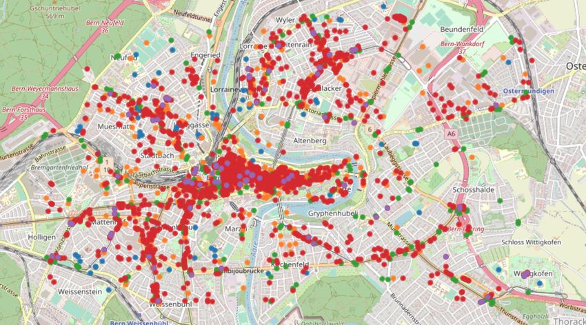
four additional regional models of other urban and rural regions in Switzerland and Germany [43–45]. These
supplementary findings confirm a similarly identifiable optimal parameter regime and demonstrate that both
the epidemiological model and the transmission parameter estimation procedure are robustly applicable to
other regional mobility models.
In the remainder of this section, we use the estimated transmission parameters for the model of Bern in all
of our experiments. We first empirically validate that, under our mobility and fitted transmission model, the
number of secondary infections caused by infectious individuals is overdispersed. Finally, we use our framework
to quantify the effects of a range of containment measures. To create a general epidemiological scenario, we
assume a small but continual influx of five untraceable exogenous exposures per 100,000 inhabitants and per
week and simulate the model state variables over a period of four months.
4.3 Overdispersion of Secondary Infections
As argued in Section 1, existing epidemiological models have predominantly built on homogeneous Poisson
transmission dynamics that fail to capture the overdispersion of secondary infections observed for COVID-19.
In addition, they do not explicitly model visits to sites where exposures occur. As a result, these models
have been of little use for studying and predicting where and when infection hotspots are most likely to
occur [6, 10, 12, 16].
In contrast, we find that, under our model, overdispersion of secondary infections can emerge naturally.
More specifically, we simulate the spread of COVID-19 under no containment measures other than the testing
of symptomatic and isolation of positively tested individuals. During these simulations, we count the number
of secondary infections caused by individuals that got infectious during during a 7-day window after 1 month
of the model simulations. Using two goodness-of-fit tests for the Poisson distribution, the Chi-squared (χ2 )
90.8 NBin(r, k) 0.8 NBin(r, k)
Empirical Empirical
Probability
Probability
0.6 0.6
r = 2.58 ± (0.31) r = 0.38 ± (0.05)
0.4 k = 0.93 ± (0.08) 0.4 k = 0.26 ± (0.02)
0.2 0.2
0.0 0.0
0 5 10 15 0 5 10 15
(a) Number of Secondary Exposures (b) Number of Secondary Exposures During a Site Visit
Figure 3: Overdispersion of Secondary Infections. Panels a) and b) show a generalized negative
binomial model fitted by maximum likelihood estimation to the secondary infections caused by an infectious
individual, overall and stratified by site visits, respectively, and averaged over 100 random realizations. The
secondary infections are counted for individuals that got infectious during a 7-day window after 1 month
of the simulation under no containment measures other than the testing of symptomatic and isolation of
positively tested individuals.
and variance tests (VT) [46, 47], we are able to reject the null hypothesis that the distribution of secondary
infections, both overall and when stratified per visit, follows a Poisson distribution. In particular, for both
distributions of secondary infections, we obtain pχ2 < 10−8 and pVT < 10−8 . With sample variance generally
significantly exceeding the sample mean, both ways of counting the number of secondary infections naturally
exhibit a higher variance than expected under the Poisson assumption and are thus overdispersed.
Building on this result, we follow recent work in the context of COVID-19 [4, 7] and measure the
degree of overdispersion by fitting a generalized negative binomial distribution NBin(r, k), an overdispersed
generalization of the Poisson, where r > 0 is the mean or reproduction number, and k is the dispersion
parameter. Figure 3 summarizes the results. Averaged over 100 random realizations, we find that the
dispersion parameter k < 1 both overall and when stratified per visit (k = 0.93 ± (0.08) and k = 0.26 ± (0.02),
respectively), evidence of substantial overdispersion [4]. We hypothesize that the higher overdispersion
observed when aggregating per visit is a direct effect of the interaction between the stochastic check-in
mobility model and our model of transmission at sites.
4.4 Efficacy of containment measures
Reducing contacts at public sites by restricting individual mobility has been one of the most prevalent
measures to counteract the spread of COVID-19 [48]. Our modeling framework allows us to faithfully
study how effective various variants of this approach are at, e.g., containing the disease, reducing peak
hospitalizations, or changing the effective reproduction number Rt over time. Instead of restricting the
mobility of the entire population or only vulnerable groups, previous work has, for instance, proposed to
divide the population into two subgroups that get isolated on alternating days [49, 50].
Figure 4 shows a comparative analysis of three of these variants: restricting the mobility of everyone,
only vulnerable groups, or one of two random subgroups on alternating days. For each variant, we consider
different levels of mobility restriction where individual check-in activity at sites in the mobility model is
reduced by between 5% and 75%. In our simulations, the vulnerable groups are defined as individuals older
than 60 years, who typically suffer more complications from COVID-19 [38, 43]. Our findings highlight the
fact that the efficacy of each policy strongly depends on the degree to which individual movement activity
is reduced. While restricting the mobility of everyone is overall clearly most effective, our findings suggest
that isolating (i.e., reducing the mobility by 100%) one of two subgroups on alternating days can reduce the
effective reproduction number, averaged over the phase of exponential case growth, and peak hospitalizations
as much as reducing the mobility of everyone by 50%. Moreover, our results also suggest that the morally
debatable strategy of quarantining only vulnerable groups does not live up to its expectation of reducing
peak hospitalizations significantly.
1025% reduced mobility 50% reduced mobility 75% reduced mobility
40000 40000 40000
30000 30000 30000
Infected
No measures
20000 20000 20000 Everyone
Alternating groups
Vulnerable groups
10000 10000 10000
0 0 0
0 50 100 0 50 100 0 50 100
t [days] t [days] t [days]
(a) Infected over time
3.0
% reduction of peak hosp.
100 Everyone
2.5 Alternating groups
80 Vulnerable groups
2.0
60
Reff
1.5
40
1.0
No measures
Everyone 20
0.5 Alternating groups
Vulnerable groups
0.0 0
0 25 50 75 100 5 25 50 75 100
% reduced mobility % reduced mobility
(b) Effective reproduction number (c) Reduction of peak hospitalizations
Figure 4: Mobility restrictions. Individuals of certain groups reduce their mobility, i.e., their frequency of
visits to sites by a certain proportion. Panel a) shows the number of infected over time for different levels
of mobility restrictions. Panel b) shows the effective reproduction number during the phase of exponential
growth of the number of infected. Panel c) shows the reduction of peak hospitalizations compared to a
scenario without mobility restrictions. Points and lines represent the mean over 100 rollouts of the simulation.
Error bars and shaded regions correspond to plus and minus one and two standard deviations respectively.
Orthogonal to various strategies that aim at reducing the number of contacts, the promise of digital
contact tracing has been to achieve fine-grained epidemic control without severe societal or economical
restrictions [24]. In this section, whenever an individual is tested positive, we use contact tracing to identify
all of their contacts in the 10 days leading up to the test result (see Section 2.4). If a given contact was longer
than 15 minutes—the time threshold used by the national COVID-19 tracing apps in, e.g., France, Germany,
Switzerland, and the United Kingdom [51–54]—the contact person is tested and isolated from everyone in
the mobility model for 14 days.
We analyze the effectiveness of digital contact tracing in combination with various degrees of mobility
restrictions for the entire population at different digital tracing adoption levels. The findings shown in
Figure 5a illustrate that the adoption of the digital tracing system and the activity reduction due to social
distancing have a complementary relationship in reducing the cumulative number of infections, as already
argued by previous work [55]. Furthermore, the results suggest that, while contact tracing can provide a
significant contribution to the mitigation of an epidemic, even at high adoption levels of 75%, it requires
combination with activity reductions of 25% and above in order to achieve epidemic control (Rt < 1). The
effective reproduction number Rt shown in Figure 5b decreases over time at a constant adoption level due to
the growing number of recovered individuals in the population.
5 Related Work
Our work builds upon previous work on compartmental epidemiological modeling, human mobility models,
and temporal point processes. Most of the classical epidemiological literature has focused on developing
11100 100 0% adoption 25% adoption
90 3 3
% adoption of contact tracing
80 80 2 2
% reduction of infections
Rt
Rt
70 1 1
60 60 0 0
60 120 60 120
50 t [days] t [days]
40 40 50% adoption 75% adoption
30 3 3
20 20 2 2
Rt
Rt
10 1 1
0
0 0 0
0 10 20 30 40 50 60 120 60 120
% reduced mobility t [days] t [days]
(a) Reduction of infections (b) Reproduction number at 10% reduced activity
0% reduced mobility 10% reduced mobility 25% reduced mobility
40000 40000 40000
30000 30000 30000 0% adoption
Infected
10% adoption
20000 20000 20000 25% adoption
50% adoption
75% adoption
10000 10000 10000
0 0 0
0 50 100 0 50 100 0 50 100
t [days] t [days] t [days]
(c) Infected over time
Figure 5: Contact tracing. A certain proportion of the population has adopted a digital contact tracing
system and, in addition, everyone reduces their visit frequency to sites by a certain proportion. Quarantine
measures are imposed on traceable individuals who have been in contact with positively tested individuals for
a minimum of 15 minutes. Panel a) shows the reduction of the cumulative number of infections compared to
a scenario without interventional measures for different adoption levels of the tracing technology and various
degrees of mobility restrictions. Panel b) shows the reproduction number over time for different adoption
levels at a fixed mobility reduction of 10%. Panel c) shows the number of infected individuals over time for
different scenarios. Lines and shaded regions represent the mean and two standard deviations computed over
100 rollouts of the simulation respectively.
population models [56], unable to capture heterogeneous transmission dynamics at the individual level.
More recently, there has been research on agent-based epidemic modeling [57–61], also in the context of
COVID-19 [23, 39, 62–66]. These models predominantly use multi-layer contact networks, discrete time,
metapopulation, or Poisson transmission rate assumptions to characterize individual infections, rather than the
frequency and duration of each individual’s visits to specific sites, as our model does. Notable exceptions are
by Aleta et al. [67], who use check-in data of real sites, yet only to configure the layers of a multi-layer contact
network, and Ferreti et al. [24], who employ a time-varying transmission rate, but average over individuals
who infect few or many others. Chang et al. [31] consider specific points of interest in US cities but only
model transmission dynamics of metapopulations of up to 3,000 people rather than among single individuals.
Ultimately, none of the above models, including these three exceptions, can be faithfully used to characterize
the dispersion of the number of individual infections during a visit, or to straightforwardly study the course
of a disease under fine-grained intervention policies such as, e.g., contact tracing or COVID-19 testing.
The literature on human mobility models has a rich history, which has been extensively reviewed by
Barcosa et al. [68]. In our experiments, the spatial distribution of visits of our event-based “check-in” mobility
12model follows the gravity model [22]. Analogous to previous COVID-19 research, these visits are synthetically
generated in each simulation [49, 69, 70]. However, our formulation is not restricted to this specific choice
and one could think of designing event-based mobility models with a spatial distribution of visits following,
e.g., the radiation model [71] or population-weighted opportunities model [72]. That said, the configuration
of visit types, frequencies, and durations are specific to event-based models as ours, where the existing body
of work on mobility models provides only very limited guidance [73, 74].
Finally, there has been a flurry of work on temporal point process modeling in the machine learning
literature in recent years [75–78]. They have been particularly successful in predicting information propagation
in social networks and the web, where they have achieved state of the art performances [79, 80]. However, the
development of compartmental epidemiological models based on temporal point processes has been lacking.
6 Discussion
Motivated by multiple lines of evidence that strongly suggest for infection hotspots to play a key role in the
transmission dynamics of COVID-19, we have introduced a spatiotemporal epidemic model that explicitly
represents sites where infections occur and hotspots may emerge. Through a case study that used fine-grained
demographic data, site locations, mobility data, as well as COVID-19 case data from Bern, Switzerland, we
have demonstrated that our model can allow individuals and policy-makers to make more effective decisions
concerning the implementation of containment measures, contact tracing, and testing at the individual level.
To facilitate this, we have released an easy-to-use implementation of the entire framework necessary to perform
experiments for any desired region [20]. While the purpose of this work does not lie in providing mechanistic
forecasts, we have shown that an identifiable pair of only two fitted parameters, the transmission rates at
sites and in households, provides reasonable predictiveness over our estimation window. Importantly, our
epidemiological model empirically exhibits overdispersion in the number of secondary infections, suggesting
that our formulation characterizes the transmission dynamics at infection hotspots—an epidemiological driver
that effective containment measures would demand preventing [10, 16].
Finally, in this work, we have used fine-grained demographic data and site locations to configure our
mobility model. However, if contact tracing data become accessible to researchers, we believe that the
variance of our predictions could be lowered and that it would be possible to use our framework to identify
areas with higher risk of infection in real time. Beyond legal compliance and gaining societal acceptance, the
use of epidemic models with high spatiotemporal resolution such as ours should respect each individual’s
privacy. In this context, it is important to highlight that, both during parameter estimation and contact
tracing, we only need to compute the contact duration of individuals with an infected person—the identity of
the infected person is not required. As a result, there are reasons to believe that such computations can be
made in a decentralized and privacy-preserving manner [81, 82]. Ultimately, although our model has greater
resolution than many of those in use today, its predictions can only be faithfully considered when being aware
of the high variance observed across random realizations.
Acknowledgements
We thank the Robert-Koch-Institute, OpenStreetMaps, Google, and Facebook for providing data to make
this work possible. We thank Brian Karrer from Facebook for his insightful comments and suggestions
regarding Bayesian optimization, Kevin Murphy, Yusef Shafi and others from Google for helpful discussions,
and Yannik Schaelte for useful comments on a preliminary version of this work. We thank Cansu Culha and
the Stanford Future Bay Initiative as well as Pavol Harar from the University of Vienna for working with us
to improve our publicly available implementation. This work was supported in part by SNSF under grant
number 200021-182407 and the European Research Council (ERC) under the European Union’s Horizon 2020
research and innovation programme (grant agreement No. 945719).
13References
[1] Johns Hopkins University & Medicine: coronavirus resource center. https://coronavirus.jhu.edu/ (2020).
[2] Adam, D. C. et al. Clustering and superspreading potential of SARS-CoV-2 infections in hong kong. Nature
Medicine 26, 1714–1719 (2020).
[3] MSF. Too little, too late: The unacceptable neglect of the elderly in care homes during the COVID-19 epidemic
in spain (2020).
[4] Endo, A. et al. Estimating the overdispersion in COVID-19 transmission using outbreak sizes outside china.
Wellcome Open Research 5 (2020).
[5] Lau, M. S. et al. Characterizing superspreading events and age-specific infectiousness of SARS-CoV-2 transmission
in georgia, usa. Proceedings of the National Academy of Sciences 117, 22430–22435 (2020).
[6] Frieden, T. & Lee, C. Identifying and interrupting superspreading events—implications for control of severe acute
respiratory syndrome coronavirus 2 (2020).
[7] Athreya, S., Gadhiwala, N. & Mishra, A. Effective reproduction number and dispersion under contact tracing
and lockdown on COVID-19 in karnataka. medRxiv (2020).
[8] The Korean clusters: How coronavirus cases exploded in south korean churches and hospitals. https://
graphics.reuters.com/CHINA-HEALTH-SOUTHKOREA-CLUSTERS/0100B5G33SB/index.html (2020).
[9] Walker, A. et al. Genetic structure of SARS-CoV-2 reflects clonal superspreading and multiple independent
introduction events, north-rhine westphalia, germany, february and march 2020. Eurosurveillance 25, 2000746
(2020).
[10] Cevik, M., Marcus, J., Buckee, C. & Smith, T. SARS-CoV-2 transmission dynamics should inform policy. SSRN
3692807 (2020).
[11] Hasan, A. et al. Superspreading in early transmissions of COVID-19 in indonesia. Scientific reports 10, 1–4
(2020).
[12] Zhang, Y., Li, Y., Wang, L., Li, M. & Zhou, X. Evaluating transmission heterogeneity and super-spreading event
of COVID-19 in a metropolis of china. International journal of environmental research and public health 17, 3705
(2020).
[13] Oh, M.-d. et al. Middle east respiratory syndrome coronavirus superspreading event involving 81 persons, korea
2015. Journal of Korean medical science 30, 1701 (2015).
[14] Lloyd-Smith, J. O., Schreiber, S. J., Kopp, P. E. & Getz, W. M. Superspreading and the effect of individual
variation on disease emergence. Nature 438, 355–359 (2005).
[15] Stein, R. A. Super-spreaders in infectious diseases. International Journal of Infectious Diseases 15, e510–e513
(2011).
[16] Althouse, B. M. et al. Stochasticity and heterogeneity in the transmission dynamics of SARS-CoV-2. arXiv
preprint arXiv:2005.13689 (2020).
[17] Brochu, E., Cora, V. M. & de Freitas, N. A tutorial on bayesian optimization of expensive cost functions, with
application to active user modeling and hierarchical reinforcement learning (2010). 1012.2599.
[18] Jones, D. R., Schonlau, M. & Welch, W. J. Efficient global optimization of expensive black-box functions. Journal
of Global optimization 13, 455–492 (1998).
[19] Snoek, J., Larochelle, H. & Adams, R. P. Practical bayesian optimization of machine learning algorithms
2951–2959 (2012).
[20] Lorch, L. et al. Data and code from “Quantifying the Effects of Contact Tracing, Testing, and Containment
Measures in the Presence of Infection Hotspots”. https://github.com/covid19-model/simulator (2020).
[21] De, A., Upadhyay, U. & Gomez-Rodriguez, M. Temporal point processes. Tech. Rep., Technical report, Saarland
University (2019).
[22] Zipf, G. K. The P 1 P 2/D hypothesis: on the intercity movement of persons. American sociological review 11,
677–686 (1946).
[23] Li, R. et al. Substantial undocumented infection facilitates the rapid dissemination of novel coronavirus (SARS-
CoV-2). Science 368, 489–493 (2020).
14[24] Ferretti, L. et al. Quantifying SARS-CoV-2 transmission suggests epidemic control with digital contact tracing.
Science 368 (2020).
[25] Van Doremalen, N. et al. Aerosol and surface stability of SARS-CoV-2 as compared with SARS-CoV-1. New
England journal of medicine 382, 1564–1567 (2020).
[26] Lauer, S. A. et al. The incubation period of coronavirus disease 2019 (COVID-19) from publicly reported
confirmed cases: estimation and application. Annals of internal medicine 172, 577–582 (2020).
[27] Linton, N. M. et al. Incubation period and other epidemiological characteristics of 2019 novel coronavirus
infections with right truncation: a statistical analysis of publicly available case data. Journal of clinical medicine
9, 538 (2020).
[28] Ahmed, N. et al. A survey of COVID-19 contact tracing apps. IEEE Access 8, 134577–134601 (2020).
[29] Aalen, O. O., Borgan, Ø. & Gjessing, H. K. Survival and Event History Analysis (Springer New York, 2008).
[30] Astudillo, R. & Frazier, P. I. Bayesian optimization of composite functions (2019). 1906.01537.
[31] Chang, S. et al. Mobility network models of COVID-19 explain inequities and inform reopening. Nature 589,
82–87 (2021).
[32] Balandat, M. et al. Botorch: Programmable bayesian optimization in pytorch (2019). 1910.06403.
[33] Wu, J. & Frazier, P. The parallel knowledge gradient method for batch bayesian optimization. In Advances in
Neural Information Processing Systems 29, 3126–3134 (Curran Associates, Inc., 2016).
[34] Frazier, P. I. A tutorial on bayesian optimization (2018). 1807.02811.
[35] Bundesamt für Statistik, Schweiz. Households. https://www.bfs.admin.ch/bfs/de/home/statistiken/
bevoelkerung/stand-entwicklung/haushalte.html (2020).
[36] Facebook Data for Good. https://dataforgood.fb.com (2020).
[37] OpenStreetMap. https://www.openstreetmap.org/ (2020).
[38] Bundesamt für Gesundheit, Schweiz. BAG COVID19 situation summary. https://www.bag.admin.ch/bag/
en/home/krankheiten/ausbrueche-epidemien-pandemien/aktuelle-ausbrueche-epidemien/
novel-cov/situation-schweiz-und-international.html (2020).
[39] Ferguson, N. M. et al. Impact of non-pharmaceutical interventions (npis) to reduce COVID-19 mortality and
healthcare demand. imperial college COVID-19 response team. Imperial College COVID-19 Response Team 20
(2020).
[40] Der Schweizerische Bundesrat. Verordnung 2 über Massnahmen zur Bekämpfung des Coronavirus (COVID-
19) (COVID-19-Verordnung 2). https://www.admin.ch/opc/de/classified-compilation/20200744/
index.html (2020).
[41] Google. COVID-19 community mobility reports. https://www.google.com/covid19/mobility/ (2021).
[42] European Center for Disease Prevention and Control. An overview of the rapid test situation for
COVID-19 diagnosis in the eu/eea. https://www.ecdc.europa.eu/sites/default/files/documents/
Overview-rapid-test-situation-for-{COVID-19}-diagnosis-EU-EEA.pdf (2020).
[43] Robert Koch-Institut (RKI). COVID19 data set. https://npgeo-corona-npgeo-de.hub.arcgis.com/
datasets/ (2020).
[44] Land Baden-Württemberg. Verordnung der Landesregierung über infektionsschützende
Massnahmen gegen die Ausbreitung des Virus SARS-Cov-2 (Corona-Verordnung).
https://www.baden-wuerttemberg.de/de/service/aktuelle-infos-zu-corona/
aktuelle-corona-verordnung-des-landes-baden-wuerttemberg/ (2020).
[45] Bundesländer der Bundesrepublik Deutschland. Corona-Regelungen in den Bundesländern. https://www.
bundesregierung.de/breg-de/themen/coronavirus/corona-bundeslaender-1745198 (2020).
[46] Cochran, W. G. Some methods for strengthening the common χ 2 tests. Biometrics 10, 417–451 (1954).
[47] Fisher, R. A. Statistical methods for research workers. In Breakthroughs in statistics, 66–70 (Springer, 1992).
[48] Islam, N. et al. Physical distancing interventions and incidence of coronavirus disease 2019: natural experiment
in 149 countries. bmj 370 (2020).
[49] Karin, O. et al. Adaptive cyclic exit strategies from lockdown to suppress COVID-19 and allow economic activity.
MedRxiv (2020).
15[50] Meidan, D., Cohen, R., Haber, S. & Barzel, B. An alternating lock-down strategy for sustainable mitigation of
COVID-19. arXiv preprint arXiv:2004.01453 (2020).
[51] Ministre des Solidarites et de la Sante. TousAntiCovid : responses a vos questions. https:
//solidarites-sante.gouv.fr/soins-et-maladies/maladies/maladies-infectieuses/
coronavirus/tousanticovid.
[52] Corona-Warn-App Team. Corona-Warn-App: Documentation. https://github.com/corona-warn-app/
cwa-documentation/.
[53] United Kingdom National Health Service. NHS COVID-19 app risk-scoring algorithm. https://covid19.nhs.
uk/risk-scoring-algorithm.html.
[54] Federal Office of Public Health, Switzerland. How the SwissCovid app issues warnings.
https://www.bag.admin.ch/bag/en/home/krankheiten/ausbrueche-epidemien-pandemien/aktuelle-ausbrueche-
epidemien/novel-cov/swisscovid-app-und-contact-tracing.html#-1674020142.
[55] Contreras, S. et al. The challenges of containing SARS-CoV-2 via test-trace-and-isolate. Nature communications
12, 1–13 (2021).
[56] Hethcote, H. W. The mathematics of infectious diseases. SIAM review 42, 599–653 (2000).
[57] Ahn, H. J. & Hassibi, B. Global dynamics of epidemic spread over complex networks. In CDC (2013).
[58] Cator, E. & Van Mieghem, P. Second-order mean-field susceptible-infected-susceptible epidemic threshold.
Physical review E (2012).
[59] Chakrabarti, D., Wang, Y., Wang, C., Leskovec, J. & Faloutsos, C. Epidemic thresholds in real networks. ACM
Transactions on Information and System Security (TISSEC) 10, 1–26 (2008).
[60] Van Mieghem, P. The N-intertwined SIS epidemic network model. Computing (2011).
[61] Van Mieghem, P., Omic, J. & Kooij, R. Virus spread in networks. IEEE/ACM TON (2009).
[62] Moghadas, S. M. et al. Projecting hospital utilization during the COVID-19 outbreaks in the united states.
Proceedings of the National Academy of Sciences 117, 9122–9126 (2020).
[63] Wells, C. R. et al. Impact of international travel and border control measures on the global spread of the novel
2019 coronavirus outbreak. Proceedings of the National Academy of Sciences 117, 7504–7509 (2020).
[64] Di Domenico, L., Pullano, G., Pullano, G., Hens, N. & Colizza, V. Expected impact of school closure and telework
to mitigate COVID-19 epidemic in france. EPIcx Lab 15 (2020).
[65] Herbrich, R., Rastogi, R. & Vollgraf, R. Crisp: A probabilistic model for individual-level COVID-19 infection
risk estimation based on contact data (2020). 2006.04942.
[66] Kucharski, A. J. et al. Effectiveness of isolation, testing, contact tracing, and physical distancing on reducing
transmission of SARS-CoV-2 in different settings: a mathematical modelling study. The Lancet Infectious Diseases
20, 1151–1160 (2020).
[67] Aleta, A. et al. Modelling the impact of testing, contact tracing and household quarantine on second waves of
COVID-19. Nature Human Behaviour 4, 964–971 (2020).
[68] Barbosa, H. et al. Human mobility: Models and applications. Physics Reports 734, 1–74 (2018).
[69] Duque, D. et al. Timing social distancing to avert unmanageable COVID-19 hospital surges. Proceedings of the
National Academy of Sciences 117, 19873–19878 (2020).
[70] Block, P. et al. Social network-based distancing strategies to flatten the COVID-19 curve in a post-lockdown
world. Nature Human Behaviour 4, 588–596 (2020).
[71] Simini, F., González, M. C., Maritan, A. & Barabási, A.-L. A universal model for mobility and migration patterns.
Nature 484, 96–100 (2012).
[72] Yan, X.-Y., Zhao, C., Fan, Y., Di, Z. & Wang, W.-X. Universal predictability of mobility patterns in cities.
Journal of The Royal Society Interface 11, 20140834 (2014).
[73] Jankowiak, M. & Gomez-Rodriguez, M. Uncovering the spatiotemporal patterns of collective social activity. In
Proceedings of the 2017 SIAM International Conference on Data Mining, 822–830 (SIAM, 2017).
[74] Zarezade, A., Jafarzadeh, S. & Rabiee, H. R. Recurrent spatio-temporal modeling of check-ins in location-based
social networks. Plos one 13, e0197683 (2018).
16You can also read