Assessing the simulated soil hydrothermal regime of the active layer from the Noah-MP land surface model (v1.1) in the permafrost regions of the ...
←
→
Page content transcription
If your browser does not render page correctly, please read the page content below
Geosci. Model Dev., 14, 1753–1771, 2021
https://doi.org/10.5194/gmd-14-1753-2021
© Author(s) 2021. This work is distributed under
the Creative Commons Attribution 4.0 License.

Assessing the simulated soil hydrothermal regime of the active layer
from the Noah-MP land surface model (v1.1) in the permafrost
regions of the Qinghai–Tibet Plateau
Xiangfei Li1,2,3 , Tonghua Wu1,3 , Xiaodong Wu1 , Jie Chen1 , Xiaofan Zhu1 , Guojie Hu1 , Ren Li1 , Yongping Qiao1 ,
Cheng Yang1,3 , Junming Hao1,3 , Jie Ni1,3 , and Wensi Ma1,3
1 Cryosphere  Research Station on the Qinghai–Tibet Plateau, State Key Laboratory of Cryospheric Science,
Northwest Institute of Eco-Environment and Resources, Chinese Academy of Sciences, Lanzhou 730000, China
2 National Cryosphere Desert Data Center, Northwest Institute of Eco-Environment and Resources,

Chinese Academy of Sciences, Lanzhou 730000, China
3 College of Resources and Environment, University of Chinese Academy of Sciences, Beijing 100049, China

Correspondence: Tonghua Wu (thuawu@lzb.ac.cn)

Received: 17 May 2020 – Discussion started: 30 June 2020
Revised: 23 February 2021 – Accepted: 24 February 2021 – Published: 30 March 2021

Abstract. Extensive and rigorous model intercomparison is         scheme would be constructive to a better understanding of
of great importance before model application due to the un-       the land surface processes in the permafrost regions of the
certainties in current land surface models (LSMs). Without        QTP as well as to further model improvements towards soil
considering the uncertainties in forcing data and model pa-       hydrothermal regime modeling using LSMs.
rameters, this study designed an ensemble of 55 296 experi-
ments to evaluate the Noah LSM with multi-parameterization
(Noah-MP) for snow cover events (SCEs), soil temperature
(ST) and soil liquid water (SLW) simulation, and investigated
the sensitivity of parameterization schemes at a typical per-     1   Introduction
mafrost site on the Qinghai–Tibet Plateau (QTP). The results
showed that Noah-MP systematically overestimates snow             The Qinghai–Tibet Plateau (QTP) is underlain by the world’s
cover, which could be greatly resolved when adopting the          largest high-altitude permafrost, covering a contemporary
sublimation from wind and a semi-implicit snow/soil tem-          area of 1.06 × 10⁶ km2 (Zou et al., 2017). Under the back-
perature time scheme. As a result of the overestimated snow,      ground of climate warming and intensifying human activi-
Noah-MP generally underestimates ST, which is mostly in-          ties, soil hydrothermal dynamics in the permafrost regions on
fluenced by the snow process. A systematic cold bias and          the QTP has been widely suffering from soil warming (Wang
large uncertainties in soil temperature remain after elimi-       et al., 2021), soil wetting (Zhao et al., 2019) and changes in
nating the effects of snow, particularly in the deep layers       the soil freeze–thaw cycle (Luo et al., 2020). Such changes
and during the cold season. The combination of roughness          have not only induced a reduction in the permafrost extent,
length for heat and under-canopy (below-canopy) aerody-           the disappearance of permafrost patches and thickening of
namic resistance contributes to resolving the cold bias in soil   the active layer (Chen et al., 2020), but they have also re-
temperature. In addition, Noah-MP generally underestimates        sulted in alterations to the hydrological cycles (Zhao et al.,
top SLW. The runoff and groundwater (RUN) process dom-            2019; Woo, 2012), changes in the ecosystem (Fountain et al.,
inates the SLW simulation in comparison to the very lim-          2012; Yi et al., 2011) and damage to infrastructure (Hjort
ited impacts of all other physical processes. The analysis of     et al., 2018). Therefore, it is very important to monitor and
the model structural uncertainties and characteristics of each    simulate the soil hydrothermal regime in order to adapt to the
                                                                  changes taking place.

Published by Copernicus Publications on behalf of the European Geosciences Union.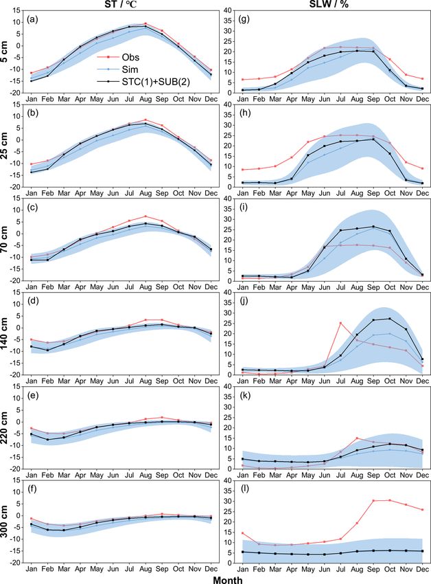
1754                              X. Li et al.: Assessment of Noah-MP LSM v1.1 for simulating soil hydrothermal regime

   A number of monitoring sites have been established in          tion schemes (Niu et al., 2011). Due to the simplicity in se-
the permafrost regions of the QTP (Cao et al., 2019). How-        lecting alternative schemes within one modeling framework,
ever, it is inadequate to construct the soil hydrothermal state   it has been attracting increasing attention in intercomparison
by considering the spatial variability of the ground thermal      work among multiple parameterizations at point and water-
regime and the uneven distribution of these observations. In      shed scales (Hong et al., 2014; Zheng et al., 2017; Gan et
contrast, numerical models are competent alternatives. In re-     al., 2019; Zheng et al., 2019; Chang et al., 2020; You et al.,
cent years, land surface models (LSMs), which describe the        2020a). For example, Gan et al. (2019) carried out an ensem-
exchanges of heat, water, and momentum between the land           ble of 288 simulations from multi-parameterization schemes
and atmosphere (Maheu et al., 2018), have received signifi-       of six physical processes, assessed the uncertainties in pa-
cant improvements with respect to the representation of per-      rameterizations in Noah-MP, and further revealed the best-
mafrost and frozen ground processes (Koven et al., 2013;          performing schemes for latent heat, sensible heat and terres-
Nicolsky et al., 2007; Melton et al., 2019). LSMs are ca-         trial water storage simulation over 10 watersheds in China.
pable of simulating the transient change in subsurface hy-        You et al. (2020b) assessed the performance of Noah-MP
drothermal processes (e.g., soil temperature and moisture)        in simulating snow process at eight sites over distinct snow
with soil heat conduction (or diffusion) and water movement       climates and identified the shared and specific sensitive pa-
equations (Daniel et al., 2008). Moreover, they could be in-      rameterizations at all sites, finding that sensitive parameter-
tegrated with a numerical weather prediction system such as       izations contribute most of the uncertainties in the multi-
WRF (Weather Research and Forecasting), making them ef-           parameterization ensemble simulations. Nevertheless, there
fective tools to explore comprehensive interactions between       is little research on the intercomparison of soil hydrother-
climate and permafrost (Nicolsky et al., 2007).                   mal processes in the permafrost regions. In this study, an en-
   Some LSMs have been evaluated and applied in the per-          semble experiment of 55 296 scheme combinations was con-
mafrost regions of the QTP. Guo and Wang (2013) investi-          ducted at a typical permafrost monitoring site on the QTP.
gated near-surface permafrost and seasonally frozen ground        The simulated snow cover events (SCEs), soil temperature
states as well as their changes using version 4 of the Com-       (ST) and soil liquid water (SLW) of the Noah-MP model
munity Land Model (CLM4). Hu et al. (2015) applied a              was assessed, and the sensitivities of the parameterization
coupled heat and mass transfer model to identify the hy-          schemes at different depths were further investigated. This
drothermal characteristics of the permafrost active layer in      study could be expected to present a reference for soil hy-
the QTP. Using an augmented Noah LSM, Wu et al. (2018)            drothermal simulation in the permafrost regions on the QTP.
modeled the extent of permafrost, the active layer thickness,        This article is structured as follows: Sect. 2 introduces the
the mean annual ground temperature, the depth of the zero         study site, the atmospheric forcing data, the design of the
annual amplitude and the ground ice content on the QTP            ensemble simulation experiments and the sensitivity analysis
in the 2010s. Despite those achievements based on differ-         methods; Sect. 3 describes the ensemble simulation results
ent models, LSMs are in many aspects insufficient in per-         of the SCEs, ST and SLW, and explores the sensitivity and
mafrost regions. For one thing, large uncertainties still exist   interactions of parameterization schemes; Sect. 4 discusses
in state-of-the-art LSMs when simulating the soil hydrother-      the schemes in each physical process, and Sect. 5 concludes
mal regime on the QTP (Chen et al., 2019). For instance, 19       the main findings.
LSMs in CMIP5 overestimate snow depth over the QTP (Wei
and Dong, 2015), which could result in variations in the soil
hydrothermal regime with respect to the aspects of magni-         2     Methods and materials
tude and vector (cooling or warming) (Zhang, 2005). More-
over, most of the existing LSMs are not originally developed      2.1    Site description and observation datasets
for permafrost regions: many of their soil processes are de-
signed for shallow soil layers (Westermann et al., 2016), but     The Tanggula observation station (TGL) lies in the contin-
permafrost occurs in the deep soil; moreover, the soil column     uous permafrost regions of the Tanggula Mountains, on the
is often considered to be homogeneous, which cannot rep-          central QTP (33.07◦ N, 91.93◦ E; 5100 m a.s.l.; Fig. 1). This
resent the stratified soil that is common on the QTP (Yang        site is a typical permafrost site on the plateau with a sub-
et al., 2005). Given the numerous LSMs and their possible         frigid and semiarid climate (Li et al., 2019), filmy and dis-
deficiencies, it is necessary to assess the parameterization      continuous snow cover (Che et al., 2019), sparse grassland
schemes for permafrost modeling on the QTP, which is help-        (Yao et al., 2011), coarse soil (Wu and Nan, 2016; He et al.,
ful for identifying the influential sub-processes, for enhanc-    2019), and thick active layer (Luo et al., 2016), which are
ing our understanding of model behavior and for guiding the       common features in the permafrost regions of the plateau.
improvement of model physics (Zhang et al., 2016).                According to the observations from 2010 to 2011, the annual
   The Noah LSM with multi-parameterization (Noah-MP)             mean air temperature of the TGL site was −4.4 ◦ C. The an-
provides a unified framework in which a given physical pro-       nual precipitation was 375 mm, 80 % of which was concen-
cess can be interpreted using multiple optional parameteriza-     trated between May and September. Alpine steppe with low

Geosci. Model Dev., 14, 1753–1771, 2021                                           https://doi.org/10.5194/gmd-14-1753-2021
X. Li et al.: Assessment of Noah-MP LSM v1.1 for simulating soil hydrothermal regime                                          1755

height is the main land surface, and this land surface type      and orthogonal experiments were carried out to evaluate their
covers about 40 %–50 % of the region (Yao et al., 2011). The     performance in soil hydrothermal dynamics.
active layer thickness is about 3.15 m (Hu et al., 2017).           The Noah-MP model was modified to consider the vertical
   The atmospheric forcing data, including wind speed and        heterogeneity in the soil profile by setting the corresponding
direction; air temperature, relative humidity and pressure;      soil parameters for each layer. The soil hydraulic parame-
downward shortwave and longwave radiation; and precipita-        ters, including the porosity, saturated hydraulic conductivity,
tion, were used to drive the model. The abovementioned vari-     hydraulic potential, the Clapp–Hornberger parameter b, the
ables were measured at a height of 2 m and covered the pe-       field capacity, the wilt point and the saturated soil water dif-
riod from 10 August 2010 to 10 August 2012 with a temporal       fusivity, were determined using the pedotransfer functions
resolution of 1 h. Daily soil temperature and liquid moisture    proposed by Hillel (1980), Cosby et al. (1984), and Wet-
at depths of 5, 25, 70, 140, 220 and 300 cm from 10 Au-          zel and Chang (1987) (Eqs. S1–S7 in the Supplement), in
gust 2010 to 9 August 2011 were utilized to validate the sim-    which the sand and clay percentages were based on Hu et
ulation results.                                                 al. (2017) (Table S1). In addition, the simulation depth was
                                                                 extended to 8.0 m to cover the active layer thickness of the
                                                                 QTP. The soil column was discretized into 20 layers (Ta-
2.2   Ensemble experiments of Noah-MP
                                                                 ble S1), whose depths follow the default scheme in CLM 5.0
                                                                 (Lawrence et al., 2018). Due to the inexact match between
The offline Noah-MP LSM v1.1 was assessed in this study.         observed and simulated depths, the simulations at 4, 26, 80,
The default Noah-MP model consists of 12 physical pro-           136, 208 and 299 cm were compared with the observations at
cesses that are interpreted by multiple optional parameter-      5, 25, 70, 140, 220 and 300 cm, respectively. A 30-year spin-
ization schemes. These sub-processes include the follow-         up was conducted in every simulation to reach equilibrium
ing: the vegetation model (VEG), canopy stomatal resistance      soil states.
(CRS), the soil moisture factor for stomatal resistance (BTR),
runoff and groundwater (RUN), the surface layer drag coef-       2.3   Methods for sensitivity analysis
ficient (SFC), supercooled liquid water (FRZ), frozen soil
permeability (INF), the canopy gap for radiation transfer        The simulated snow cover events (SCEs) were quantitatively
(RAD), snow surface albedo (ALB), the precipitation par-         evaluated using the overall accuracy index (OA) (Toure et al.,
tition (SNF), the lower boundary of soil temperature (TBOT)      2016):
and the snow/soil temperature time scheme (STC) (Table 1).                a+d
Details about the processes and optional parameterizations       OA =           ,                                               (1)
                                                                        a+b+c+d
can be found in Yang et al. (2011a).
    VEG(1) is adopted in the VEG process, in which               where a represents the positive hits, b represents the false
the vegetation fraction is prescribed according to the           alarm, c represents the misses and d represents the negative
NESDIS/NOAA 0.144 degree monthly 5-year climatol-                hits. The value of the OA ranges from 0 to 1. A higher OA
ogy green vegetation fraction (https://ral.ucar.edu/solutions/   signifies better performance. Ground albedo was used as an
products/wrf-noah-noah-mp-modeling-system, last access:          indicator for snow events due to a lack of snow depth obser-
27 March 2021), and the monthly leaf area index (LAI)            vations. The days when the daily mean albedo is greater than
was derived from the Advanced Very High-Resolution Ra-           the observed mean value of the warm and cold season (0.25
diometer (AVHRR; https://www.ncei.noaa.gov/data/, last ac-       and 0.30, respectively) are identified as snow cover.
cess: 27 March 2021, Claverie et al., 2016). Previous stud-          The root mean square errors (RMSEs) between the simu-
ies have confirmed that Noah-MP seriously overestimates the      lations and observations were adopted to evaluate the perfor-
snow events and underestimates soil temperature and mois-        mance of Noah-MP in simulating soil hydrothermal dynam-
ture on the QTP (Jiang et al., 2020; Li et al., 2020; Wang       ics.
et al., 2020), which can be greatly resolved by considering          To investigate the degree of influence of each physical pro-
the sublimation from wind (Gordon scheme) and a combina-         cess on the SCEs, ST and SLW, we firstly calculated the
tion of roughness length for heat and under-canopy (below-       mean OA (for SCE) and the mean RMSE (for ST and SLW)
canopy) aerodynamic resistance (Y08–UCT scheme) (Zeng            (Ȳji ) of the j th parameterization schemes (j = 1, 2, . . . ) in
et al., 2005; Yang et al., 2008; Li et al., 2020). For a more    the ith process (i = 1, 2, . . . ). The maximum difference in
comprehensive assessment, we added two physical processes        Ȳji (1OA or 1RMSE) was then defined to quantify the de-
based on the default Noah-MP model – i.e., the snow subli-       gree of influence of the ith process (i = 1, 2, . . . ) (Li et al.,
mation from wind (SUB) and the combination scheme pro-           2015):
cess (CMB) (Table 1). In the two processes, users can choose                      i
                                                                 1OA or 1RMSE = Ȳmax     i
                                                                                      − Ȳmin ,                                 (2)
to turn on the respective Gordon and Y08–UCT schemes (de-
scribed in the study of Li et al., 2020) or not. As a result,            i
                                                                 where Ȳmax        i are the largest and the smallest Ȳ i in the
                                                                              and Ȳmin                                  j
55 296 total combinations are possible for the 13 processes,     ith process, respectively. For a given physical process, a high

https://doi.org/10.5194/gmd-14-1753-2021                                            Geosci. Model Dev., 14, 1753–1771, 2021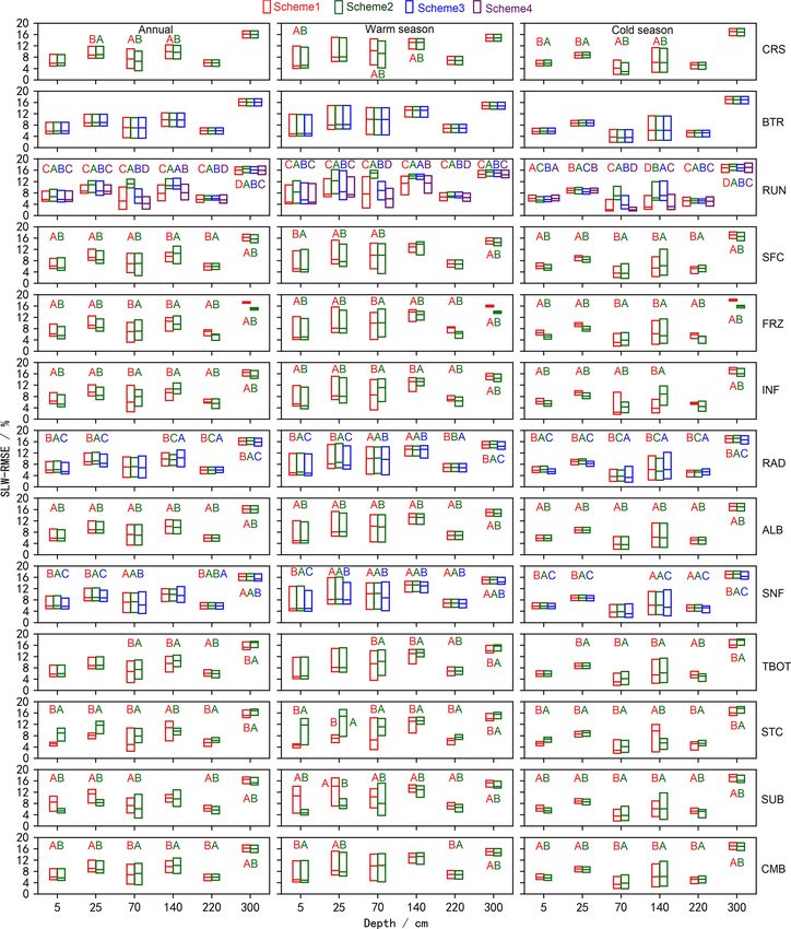
1756 X. Li et al.: Assessment of Noah-MP LSM v1.1 for simulating soil hydrothermal regime
Figure 1. Location and geographic features of the study site. (a) Location of the observation site and permafrost distribution (Zou et al.,
2017). (b) Topography of the Qinghai–Tibet Plateau. (c) Photo of the Tanggula observation station.
1OA or 1RMSE signifies a large difference between param- albedo was used as an indicator of snow cover. Figure 2
eterizations, indicating high sensitiveness of the ith process shows the monthly variations in observed ground albedo
for SCEs and ST/SLW simulation. and the simulation results of the ensemble simulations. The
The sensitivities of physical processes were determined ground albedo was extremely overestimated with large un-
by quantifying the statistical distinction level of performance certainties when considering the snow options in Noah-MP,
between parameterization schemes. The independent sample indicating an overestimation of snow depth and duration.
(two-tailed) t test was adopted to identify whether the dis- This overestimation continued until July.
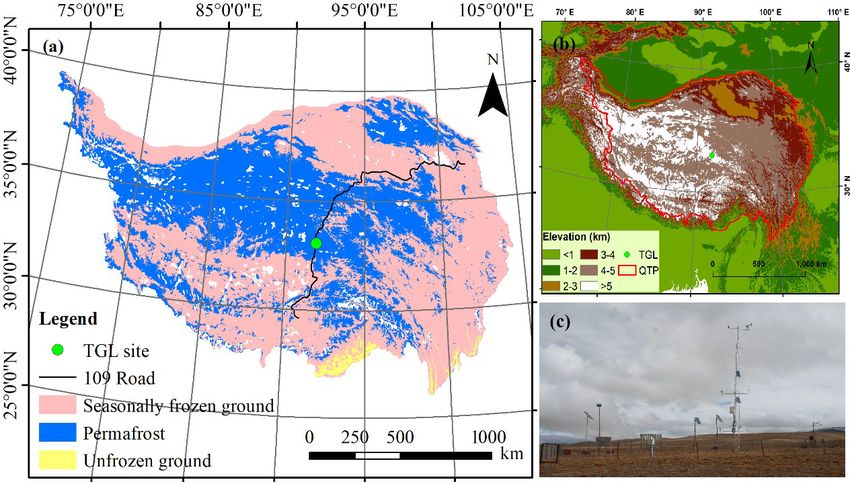
tinction level between two schemes was significant, and the Figure 3 illustrates the ensemble-simulated and observed
significance of the distinction level between three or more annual cycle of ST and SLW at the TGL site. The ensem-
schemes was tested using a Tukey test. The Tukey test has ble experiments basically captured the seasonal variability of
been widely used due to its simple computation and statisti- ST, whose magnitude decreased with soil depth. In addition,
cal features (Benjamini, 2010). Detailed descriptions of this the simulated ST in the snow-affected season (October–July)
method can be found in Zhang et al. (2016), Gan et al. (2019) showed relatively wide uncertainty ranges, particularly in the
and You et al. (2020a). A process can be considered sensitive shallow layers. This indicates that the selected schemes per-
when the schemes show a significant difference. Moreover, form very differently with respect to snow simulation, result-
schemes with a large mean OA and a small mean RMSE ing in large uncertainties in shallow STs. The simulated ST
were considered favorable for SCEs and ST/SLW simulation, were generally smaller than the observations with relatively
respectively. We distinguished the differences of the param- large gaps during the snow-affected season. This indicates
eterization schemes at the 95 % confidence level. that the Noah-MP model generally underestimates the ST,
especially during the snow-affected months.
As the observation equipment can only record the liquid
3 Results water, the soil liquid water (SLW) was evaluated against sim-
ulations from the ensemble experiments (Fig. 3). The Noah-
3.1 General performance of the ensemble simulation
MP model generally underestimated surface (5 and 25 cm)
The performance of Noah-MP for snow simulation was and deep (220 and 300 cm) SLW (Fig. 3g, h, k, l). However,
firstly tested by conducting an ensemble of 55 296 experi- Noah-MP tended to overestimate the SLW in the middle lay-
ments. Due to a lack of snow depth measurements, ground ers of 70 and 140 cm. Moreover, the simulated SLW exhib-
Geosci. Model Dev., 14, 1753–1771, 2021 https://doi.org/10.5194/gmd-14-1753-2021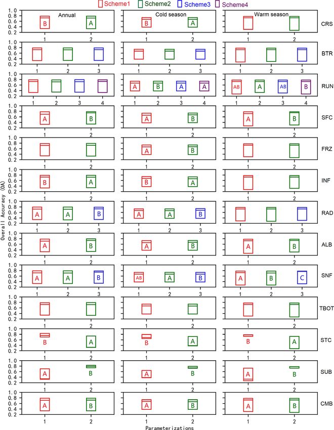
X. Li et al.: Assessment of Noah-MP LSM v1.1 for simulating soil hydrothermal regime                                                          1757

Table 1. The physical processes and options in the Noah-MP LSM (Yang et al., 2011a).

                 Physical processes                                              Options
                 Vegetation model (VEG)                                          (1) Table LAI, prescribed vegetation fraction
                                                                                 (2) Dynamic vegetation
                                                                                 (3) Table LAI, calculated vegetation fraction
                                                                                 (4) Table LAI, prescribed max vegetation fraction
                 Canopy stomatal resistance (CRS)                                (1) Jarvis
                                                                                 (2) Ball–Berry
                 Soil moisture factor for stomatal resistance (BTR)              (1) Noah
                                                                                 (2) CLM
                                                                                 (3) SSiB
                 Runoff and groundwater (RUN)                                    (1) SIMGM with groundwater
                                                                                 (2) SIMTOP with equilibrium water table
                                                                                 (3) Noah (free drainage)
                                                                                 (4) BATS (free drainage)
                 Surface layer drag coefficient (SFC)                            (1) Monin–Obukhov (M–O)
                                                                                 (2) Chen97
                 Supercooled liquid water (FRZ)                                  (1) Generalized freezing-point depression
                                                                                 (2) Variant freezing-point depression
                 Frozen soil permeability (INF)                                  (1) Defined by soil moisture, more permeable
                                                                                 (2) Defined by liquid water, less permeable
                 Canopy gap for radiation transfer (RAD)                         (1) Gap = F(3D structure, solar zenith angle)
                                                                                 (2) Gap = zero
                                                                                 (3) Gap = 1− vegetated fraction
                 Snow surface albedo (ALB)                                       (1) BATS
                                                                                 (2) CLASS
                 Precipitation partition (SNF)                                   (1) Jordan91
                                                                                 (2) BATS: Tsfc < Tfrz + 2.2 K
                                                                                 (3) Tsfc < Tfrz
                 Lower boundary of soil temperature (TBOT)                       (1) Zero heat flux
                                                                                 (2) Soil temperature at 8 m depth
                 Snow/soil temperature time scheme (STC)                         (1) Semi-implicit
                                                                                 (2) Fully implicit
                 Snow sublimation from wind (SUB)                                (1) No
                                                                                 (2) Yes
                 Combination scheme by Li et al. (2020) (CMB)                    (1) No
                                                                                 (2) Yes
               The abbreviations used in the table are as follows: BATS (Biosphere–Atmosphere Transfer Model), CLASS (Canadian Land Surface
               Scheme), SIMGM (Simple topography-based runoff and Groundwater Model), SIMTOP (Simple Topography-based hydrological
               model) and SSiB (Simplified Simple Biosphere model).

ited relatively wide uncertainty ranges, particularly during                      3.2      Sensitivity of physical processes
the warm season (Fig. 3).
                                                                                  3.2.1     Degree of influence of physical processes

                                                                                  Figure 4 compares the influence scores of the 13 physical
                                                                                  processes based on the maximum difference in the mean OA
                                                                                  over 55 296 experiments using the same scheme, for SCEs at
                                                                                  the TGL site. On the whole, the SUB and STC processes had

https://doi.org/10.5194/gmd-14-1753-2021                                                                 Geosci. Model Dev., 14, 1753–1771, 2021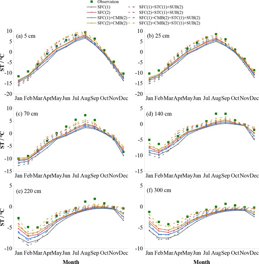
1758 X. Li et al.: Assessment of Noah-MP LSM v1.1 for simulating soil hydrothermal regime
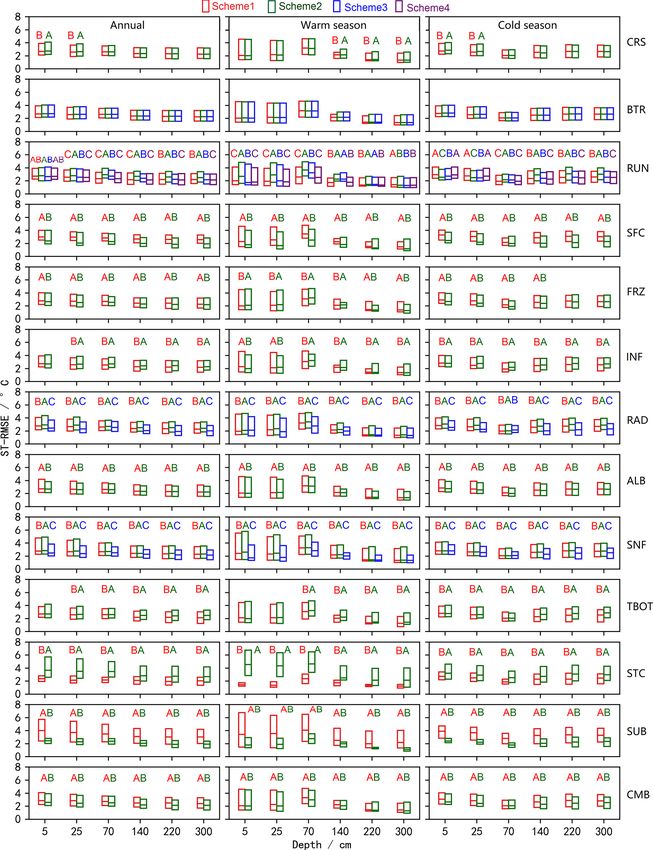
and CMB showed the smallest effects (Fig. 5b, d, f). Dur-
ing the warm season, the RUN process, along with the STC
and SUB processes, dominated the performance of SLW sim-
ulation, especially in the shallow layers (5, 25 and 70 cm;
Fig. 5d). During the cold season, however, the RUN process
dominated the SLW simulation, with a great decline in the
dominance of STC and SUB processes.
3.2.2 Sensitivities of physical processes and the general
behaviors of parameterizations
To further investigate the sensitivity of each process and
the general performance of the parameterizations, an inde-
pendent sample (two-tailed) t test and a Tukey test were
conducted to establish whether the differences between pa-
rameterizations within a physical process were significant
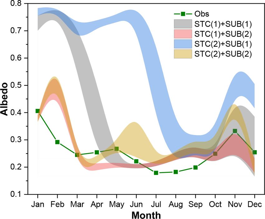
Figure 2. Monthly variations in ground albedo at the TGL site for
the observations (Obs) and the ensemble simulation (Sim). The light
(Figs. 6, 7). For a given sub-process, any two schemes la-
blue shading represents the standard deviation of the ensemble sim- beled with different letters behave significantly differently,
ulation. and this sub-process can, therefore, be identified as sensitive;
otherwise, the sub-process is considered insensitive. For sim-
plicity, schemes with insensitive sub-process are not labeled.
the largest scores for the whole year as well as during both Moreover, schemes with the letters late in the alphabet have
the warm and cold seasons, and the other processes showed smaller mean RMSEs and outperform those with letters that
a value of less than 0.05 (Fig. 4a, b, c). Moreover, the SUB appear early in the alphabet. The following outlines an exam-
process had a consistent influence on SCEs, whereas the in- ple of this process using the two schemes in the CRS process,
fluence of STC differed with season. In the cold season, the hereafter CRS(1) and CRS(2), in Fig. 6. For the annual and
score of the SUB process (0.28) was 2 times more than that of warm season, CRS(1) and CRS(2) were labeled with “B” and
the STC process (Fig. 4b), indicating the relative importance “A”, respectively. In the cold season, neither of them were
of snow sublimation for SCE simulation during the cold sea- labeled with letters. As described above, the CRS process
son. When it came to the warm season, the influence score was sensitive for SCE simulation during the annual and warm
of SUB (0.25) did not change much, whereas that of STC in- season, and CRS(1) outperformed CRS(2). However, it was
creased to 0.26 and showed a similar influence on SCE sim- not sensitive during the cold season.
ulation to SUB. Consistent with the degrees of influence shown in Fig. 4,
Figure 5 compares the influence scores of the 13 phys- the performance difference between schemes of the STC
ical processes at different soil depths, based on the maxi- and SUB processes for SCE simulation were significantly
mum difference in the mean RMSE over 55 296 experiments greater than for other processes. Most other physical pro-
using the same scheme, for ST and SLW at the TGL site. cesses showed significant but limited differences. Schemes
The snow-related processes, including the STC, SUB and in the BTR and TBOT processes, however, showed no sig-
SNF processes, showed the largest ST-1RMSE at all lay- nificant difference with respect to performance. Specifically,
ers, followed by the RAD, SFC and RUN processes, whereas the performance order was as follows: STC(1) > STC(2),
the ST-1RMSE values of the other seven physical processes SUB(2) > SUB(1), SFC(2) > SFC(1), ALB(2) > ALB(1)
were less than 0.5 ◦ C, among which the influence of the CRS and CMB(2) > CMB(1) at both the annual and seasonal
and BTR processes were negligible. Moreover, the FRZ, INF scales. RAD showed no obvious difference during the
and TBOT processes had larger influence scores during the warm season, whereas RAD(3) outperformed RAD(1) and
cold season than during the warm season, and the scores of RAD(2) during the cold season. For SNF, SNF(3) generally
TBOT were greater in deep soils than shallow soils. During excelled over SNF(1) and SNF(2), especially during the
the warm season, the physical processes generally showed warm season.
more influence on shallow soil temperatures. When it came All of the physical processes showed sensitivities for ST
to the cold season, the influence of the physical processes on and SLW simulation to varying magnitudes except for the
deep layers obviously increased and was comparable to that BTR and CRS processes in most layers. For ST, the per-
on shallow layers, implying relatively higher uncertainties in formance difference between schemes of the STC, SUB
Noah-MP during the cold season. and SNF processes were obviously greater than other pro-
Most of the 1RMSE values for SLW are less than 5 %, cesses, indicating the importance of snow on ST, followed
indicating that all of the physical processes have limited in- by the RAD, SFC and RUN processes. The performance
fluence on the SLW, among which CRS, BTR, ALB, SNF order was as follows: STC(1) > STC(2), SUB(2) > SUB(1),
Geosci. Model Dev., 14, 1753–1771, 2021 https://doi.org/10.5194/gmd-14-1753-2021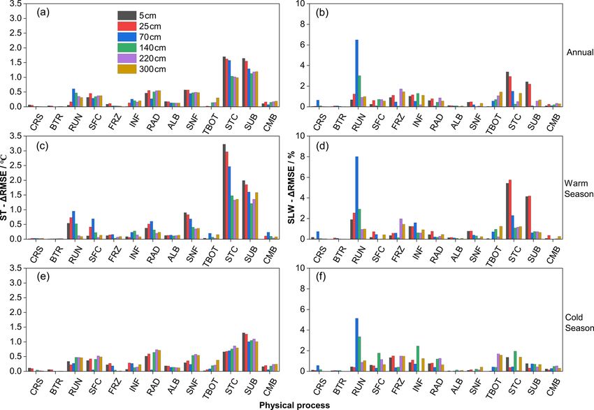
X. Li et al.: Assessment of Noah-MP LSM v1.1 for simulating soil hydrothermal regime                                                      1759

Figure 3. Monthly soil temperature (ST, in ◦ C) and soil liquid water (SLW, in %) at (a, g) 5 cm, (b, h) 25 cm, (c, i) 70 cm, (d, j) 140 cm, (e,
k) 220 cm and (f, l) 300 cm at the TGL site. The light blue shading represents the standard deviation of the ensemble simulation. The black
line and the symbols represent the ensemble mean of simulations with STC(1) and SUB(2).

SNF(3) > SNF(1) > SNF(2), RAD(3) > RAD(1) > RAD(2)                        SUB(2) > SUB(1). For the RUN process, the performance
and SFC(2) > SFC(1). For SLW, the RUN, STC and                            order for both ST and SLW simulation generally followed
SUB processes showed significant and higher sensitivi-                    RUN(4) > RUN(1) > RUN(3) > RUN(2) as a whole, among
ties than other physical processes, especially during the                 which RUN(1) and RUN(4) showed similar performance
warm season and in the shallow layers (Figs. 5, 8). Con-                  during both warm and cold seasons. During both warm and
sistent with that of ST, the performance order for the                    cold seasons, the performance order for the ST simulations
SLW simulation was as follows: STC(1) > STC(2) and                        was SFC(2) > SFC(1) for SFC process, FRZ(2) > FRZ(1)

https://doi.org/10.5194/gmd-14-1753-2021                                                       Geosci. Model Dev., 14, 1753–1771, 2021
1760                               X. Li et al.: Assessment of Noah-MP LSM v1.1 for simulating soil hydrothermal regime

Figure 4. The maximum difference in the mean overall accuracy (OA) for albedo (ALB-1OA) in each physical process (a) annually and
during the (b) cold and (c) warm seasons at the TGL site.

Figure 5. The maximum difference in the mean RMSE for (a, c, e) soil temperature (ST-1RMSE, in ◦ C) and (b, d, f) soil liquid water
(SLW-1RMSE, in %) in each physical process (a, b) annually and during the (c, d) warm and (e, f) cold seasons at different soil depths at
the TGL site.

for FRZ process and RAD(3) > RAD(1) > RAD(2) for RAD                   shallow soils during the warm season, whereas its perfor-
process (Figs. S2, S3), which is somewhat similar to SLW               mance was worse during the cold season compared with
simulations in the shallow and deep layers.                            FRZ(2) / INF(1). For SLW, FRZ(2) / INF(2) generally pre-
   For ST, both FRZ and INF showed higher sensitivi-                   ceded FRZ(1) / INF(1) in shallow and deep soils (5, 25, 220
ties during the cold season, especially in shallow soils for           and 300 cm), whereas its performance was worse in the mid-
FRZ and deep soils for INF. FRZ(2) / INF(1) outperformed               dle soil layers (140 and 220 cm).
FRZ(1) / INF(2) for the whole year with respect to ST sim-                For ST simulation, the performance sequence for
ulation. Specifically, FRZ(1) / INF(2) performed better in             RAD and SNF was RAD(3) > RAD(1) > RAD(2) and

Geosci. Model Dev., 14, 1753–1771, 2021                                                 https://doi.org/10.5194/gmd-14-1753-2021
X. Li et al.: Assessment of Noah-MP LSM v1.1 for simulating soil hydrothermal regime                                            1761

Figure 6. Distinction level for overall accuracy (OA) of snow cover events (SCEs) annually and during the warm and cold seasons at the
TGL site. The limits of the boxes represent the upper and lower quartiles, and the lines in the boxes indicate the median values.

https://doi.org/10.5194/gmd-14-1753-2021                                                Geosci. Model Dev., 14, 1753–1771, 2021
1762                             X. Li et al.: Assessment of Noah-MP LSM v1.1 for simulating soil hydrothermal regime

SNF(3) > SNF(1) > SNF(2), respectively. For SLW simula-          (5 and 25 cm), resulting in good agreement of deep STs with
tion, the sequence became complicated. However, RAD(3)           observations. In contrast, the simulated STs in the shallow
and SNF(3) still outperformed the other two schemes, re-         layers (5 and 25 cm) by SFC(1) and SFC(1) + CMB(2) were
spectively. ALB(2) was superior to ALB(1) for both ST            basically consistent with observations from March to July,
and SLW simulation. The influence of TBOT on soil hy-            whereas a large cold bias remained in the deep layers.
drothermal dynamics arose in deep soils and during cold sea-
son, and TBOT(1) excelled over TBOT(2). CMB(2) outper-
formed CMB(1) for ST simulation and for SLW simulation
in shallow and deep soils (5, 25 and 300 cm).
                                                                 4     Discussion
3.3    Influence of snow cover and the surface drag
       coefficient on soil hydrothermal dynamics                 4.1    Snow cover on the QTP and its influence on the soil
                                                                        hydrothermal regime
The influence of snow on soil temperature is firstly inves-
tigated. The dominant role of STC and SUB in the sim-            Snow cover in the permafrost regions of the QTP is thin,
ulation of SCEs has been identified (Figs. 4, 6). Interac-       patchy and short-lived (Che et al., 2019), and its influence
tions between the two physical processes are further ana-        on soil temperature and the permafrost state is usually con-
lyzed here. Figure 9 compares the uncertainly intervals of the   sidered weak (Jin et al., 2008; Zou et al., 2017; Wu et al.,
two physics. The duration of snow cover is the longest when      2018; Zhang et al., 2018; Yao et al., 2019). However, our
STC(2) + SUB(1), followed by when STC(1) + SUB(1).               ensemble simulations showed that the surface albedo is ex-
Simulations considering SUB(2) generally have a short snow       tremely overestimated with respect to both magnitude and
duration. Among the four combinations, STC(1) + SUB(2) is        duration (Fig. 2), implying an extreme overestimation of
in best agreement with the measurements.                         snow cover, which is consistent with studies using Noah-MP
   Given the good performance of STC(1) + SUB(2) in sim-         model (Jiang et al., 2020; Li et al., 2020; Wang et al., 2020)
ulating SCEs, the influence of snow on soil hydrothermal dy-     and widely found in other state-of-the-art LSMs (Wei and
namics is investigated by comparing the total ensemble mean      Dong, 2015) for the QTP.
ST and SLW with those adopting STC(1) + SUB(2) (Fig. 3).            Great efforts to resolve the overestimation of snow cover
It can be seen that the ensemble mean ST values of simula-       in LSMs include considering the vegetation effect (Park et
tions adopting STC(1) and SUB(2) are generally higher than       al., 2016), the snow cover fraction (Jiang et al., 2020), blow-
the total ensemble means, especially during the spring and       ing snow (Xie et al., 2019) and the fresh snow albedo (Wang
summer (March–August). In January and February in the            et al., 2020). Our results illustrated the superiority of consid-
shallow layers (5, 25 and 70 cm), STC(1) + SUB(2) had a          ering the snow sublimation from wind (SUB(2)) and using a
lower ST and showed an insulation effect on ST for these         semi-implicit snow/soil temperature time scheme (STC(1))
2 months. As a whole, however, snow cover has a cooling          (Figs. 4, 6, 9) when simulating snow cover on the QTP.
effect on ST. In addition, along with the improved SCEs and      This is consistent with previous conclusions that account-
elevated ST, STC(1) + SUB(2) induced moister soil with a         ing for the loss resulting from wind contributes to improving
higher SLW (Fig. 3).                                             the snow cover days and depth (Yuan et al., 2016) and that
   The SFC and CMB processes use different ways of calcu-        STC(1) has more rapid snow ablation than STC(2) (You et
lating the surface drag coefficient, which greatly influences    al., 2020a).
the surface energy partitioning and, thus, the ST and SLW.          The impacts of snow cover on soil temperature with re-
The influence of the surface drag coefficient is assessed by     spect to magnitude and vector (cooling or warming) depend
comparing the soil temperature before and after considering      on its timing, duration and depth (Zhang et al., 2005). In
the combined scheme, CMB(2), and the effect of snow,             January and February, the ground heat flux mainly goes up-
STC(1) + SUB(2) (Fig. 10). SFC(2) tended to produce a            ward, and the warming effect of simulated snow can be re-
higher ST than SFC(1), especially during the warming             lated to the overestimated snow depth that prevents heat loss
period (January–August). When adopting the combined              from the ground. During the spring and summer, when snow
Y08–UCT scheme, CMB(2), the cold bias was signifi-               melts, a cooling effects occurs, mainly because the consid-
cantly resolved. The performance order was as follows:           erable energy that is used to heat the ground is reflected
SFC(2) + CMB(2) > SFC(2) > SFC(1) + CMB(2) > SFC(1).             due to the high albedo of snow. With the improvement of
However, considerable underestimations of ST still exist in      snow (STC(1) + SUB(2)), the originally overestimated snow
all layers due to the poor representation of snow process. Af-   melts and infiltrates into the soil, resulting in improved SLWs
ter eliminating the effects of snow (STC(1) + SUB(2), dash       (Fig. 3). A higher soil temperature also contributed to the
lines in Fig. 10), the simulated ST increased accordingly, ex-   SLWs according to the freezing-point depression equation,
cept in January and February. SFC(2) and SFC(2) + CMB(2)         in which SLW exponentially increases with soil temperature
overestimated STs from March to July in the shallow layers       for a given site (Niu and Yang, 2006).

Geosci. Model Dev., 14, 1753–1771, 2021                                             https://doi.org/10.5194/gmd-14-1753-2021
X. Li et al.: Assessment of Noah-MP LSM v1.1 for simulating soil hydrothermal regime 1763 Figure 7. Distinction level for the RMSE of ST at different layers annually and during the warm and cold seasons in the ensemble simulations at the TGL site. Limits of the boxes represent the upper and lower quartiles, and the lines in the boxes indicate the median values. https://doi.org/10.5194/gmd-14-1753-2021 Geosci. Model Dev., 14, 1753–1771, 2021
1764                               X. Li et al.: Assessment of Noah-MP LSM v1.1 for simulating soil hydrothermal regime

Figure 8. Same as in Fig. 7 but for SLW.

4.2     Discussions on the sensitivity of physical processes     and SLW through its cooling effect (Shen et al., 2015) and the
        to soil hydrothermal simulation                          water balance in the root zone (Chang et al., 2020). However,
                                                                 the annual transpiration of the alpine steppe is weak due to
4.2.1    Canopy stomatal resistance (CRS) and soil               the shallow effective root zone and lower stomatal control in
         moisture factor for stomatal resistance (BTR)           this dry environment (Ma et al., 2015), which may explain
                                                                 the indistinctive or very small difference among the schemes
                                                                 of the BTR and CRS processes for SCEs (Fig. 6), ST (Fig. 7)
The biophysical BTR and CRS processes directly affect the
                                                                 and SLW (Fig. 8).
canopy stomatal resistance and, thus, plant transpiration (Niu
et al., 2011). The transpiration of plants could impact the ST

Geosci. Model Dev., 14, 1753–1771, 2021                                          https://doi.org/10.5194/gmd-14-1753-2021
X. Li et al.: Assessment of Noah-MP LSM v1.1 for simulating soil hydrothermal regime 1765
4.2.3 Surface layer drag coefficient (SFC and CMB)
SFC defines the calculation of the surface exchange coef-
ficient for heat and water vapor (CH), which greatly im-
pact the energy and water balance and, thus, the tempera-
ture and moisture of soil (Zeng et al., 2012; Zheng et al.,
2012). SFC(1) adopts the Monin–Obukhov similarity theory
(MOST) in its general form, whereas SFC(2) uses the im-
proved MOST modified by Chen et al. (1997). In SFC(1),
the roughness length for heat (Z0h ) is taken as the same as
the roughness length for momentum (Z0m ; Niu et al., 2011).
SFC(2) adopts the Zilitinkevich approach for Z0h calcula-
tion (Zilitinkevich, 1995). The difference between SFC(1)
and SFC(2) has a great impact on the CH value. Several stud-
ies have reported that SFC(2) shows better performance for
the simulation of sensible and latent heat on the QTP (Zhang
et al., 2016; Gan et al., 2019). The results of the t test in
Figure 9. Uncertainty interval of ground albedo at the TGL site in this study showed remarkable distinctions between the two
the dominant physical processes (STC and SUB) for SCE simula- schemes, where SFC(2) was dramatically superior to SFC(1)
tion. (Figs. 7, 8). SFC(2) produces lower CH values than SFC(1)
(Zhang et al., 2014), resulting in less efficient ventilation and
greater heating of the land surface (Yang et al., 2011b) as
4.2.2 Runoff and groundwater (RUN) well as a substantial improvement in the cold bias of Noah-
MP in this study (Figs. 7, 10).
In the warm season, different SLWs would result in a dif-
Both SFC(1) and SFC(2) could not produce the diurnal
ference in the surface energy partitioning and, thus, differ-
variation in Z0h (Chen et al., 2010). CMB offers a scheme
ent soil temperatures. RUN(2) had the worst performance for
that considers the diurnal variation in Z0h in bare ground
simulating ST and SLW (Figs. 7, 8) among the four schemes,
and under-canopy turbulent exchange in sparse vegetated
likely due to its higher estimation of soil moisture (Fig. S1)
surfaces (Li et al., 2020). Consistent with previous studies
and, thus, greater sensible heat and smaller ST (Gao et al.,
on the QTP (Chen et al., 2010; Guo et al., 2011; Zheng et al.,
2015). Likewise, RUN(4) was on par with RUN(1) with re-
2015; Li et al., 2020), the simulated ST generally followed
spect to the simulation of ST in most layers due to the very
SFC(2) + CMB(2) > SFC(2) > SFC(1) + CMB(2) > SFC(1)
small difference in the SLW of the two schemes (Figs. 8,
with/without removing the overestimation of snow (Fig. 10),
S1). For the whole soil column, RUN(4) surpassed RUN(1)
indicating that CMB(2) contributes to resolving the cold
and RUN(2) for SLW simulation, both of which define sur-
bias of the LSMs. However, none of the four combina-
face and subsurface runoff as functions of the groundwater
tions could satisfactorily reproduce the shallow and deep
table depth (Niu et al., 2005, 2007). This is in keeping with
STs simultaneously. When the snow was well-simulated,
the study of Zheng et al. (2017), which found that soil-water-
SFC(2) + CMB(2) performed the best in the deep layers
storage-based parameterizations outperformed groundwater-
at the cost of overestimating the shallow STs. Meanwhile,
table-based parameterizations in simulating the total runoff
SFC(1) + CMB(1) showed the best agreement in the shallow
in a seasonally frozen and high-altitude Tibetan river. More-
layers with a considerable cold bias in the deep layers, which
over, RUN(4) is designed based on the infiltration-excess
could be related to the overestimated frozen soil thermal
runoff (Yang and Dickinson, 1996) in spite of the saturation-
conductivity (Luo et al., 2009; Chen et al., 2012; Li et al.,
excess runoff in RUN(1) and RUN(2) (Gan et al., 2019),
2019).
which is more common in arid and semiarid areas like the
permafrost regions of the QTP (Pilgrim et al., 1988). In the
4.2.4 Supercooled liquid water (FRZ) and frozen soil
cold season, much of the liquid water freezes into ice, which
permeability (INF)
would greatly influence the thermal conductivity of frozen
soil considering that the thermal conductivity of ice is nearly
FRZ and INF describe the unfrozen water and permeability
4 times that of the equivalent liquid water. Therefore, the im-
of frozen soil, and they had a larger influence on ST and
pact of RUN is important for the soil temperature simulations
SLW during the cold season than during the warm season,
in both the warm and cold seasons (Figs. 5, 7).
as expected (Fig. 5). Specifically, FRZ treats liquid water in
frozen soil (supercooled liquid water) using two forms of the
freezing-point depression equation. FRZ(1) takes a general
form (Niu and Yang, 2006), whereas FRZ(2) exhibits a vari-
https://doi.org/10.5194/gmd-14-1753-2021 Geosci. Model Dev., 14, 1753–1771, 20211766 X. Li et al.: Assessment of Noah-MP LSM v1.1 for simulating soil hydrothermal regime
Figure 10. Monthly soil temperature (ST, in ◦ C) at (a) 5 cm, (b) 25 cm, (c) 70 cm, (d) 140 cm, (e) 220 cm and (f) 300 cm for the SFC process
with or without consideration of the CMB(2) and STC(1) + SUB(2) processes.
ant form that considers the increased surface area of icy soil RAD(1) defines the canopy gap as a function of the 3D veg-
particles (Koren et al., 1999). FRZ(2) generally yields more etation structure and the solar zenith angle, RAD(2) employs
liquid water compared with FRZ(1) (Fig. S2). INF(1) uses no gap within canopy and RAD(3) treats the canopy gap from
soil moisture (Niu and Yang, 2006), whereas INF(2) employs unity minus the vegetation fraction (Niu and Yang, 2004).
only the liquid water (Koren et al., 1999) to parameterize soil The RAD(3) scheme allows the most solar radiation to pen-
hydraulic properties. INF(2) generally produces more imper- etrate to the ground, followed by the RAD(1) and RAD(2)
meable frozen soil than INF(1), which is also found in this schemes. As it is an alpine grassland, there is a relative low
study (Fig. S3). For the whole year, INF(1) surpassed INF(2) LAI at the TGL site and, thus, quite a high canopy gap.
with respect to simulating STs, which may be related to the Therefore, schemes with a larger canopy gap could realisti-
more realistic SLWs produced by INF(1) for the whole soil cally reflect the environment. Consequently, the performance
column (Fig. S3). decreased in the following order for the ST and SLW simu-
lation: RAD(3) > RAD(1) > RAD(2).
4.2.5 Canopy gap for radiation transfer (RAD)
RAD treats the radiation transfer process within the vegeta-
tion and adopts three methods to calculate the canopy gap.
Geosci. Model Dev., 14, 1753–1771, 2021 https://doi.org/10.5194/gmd-14-1753-2021X. Li et al.: Assessment of Noah-MP LSM v1.1 for simulating soil hydrothermal regime 1767
4.2.6 Snow surface albedo (ALB) and precipitation STC(1) and STC(2) were significant (Fig. 7). The impacts of
partition (SNF) the two options on ST are remarkable (Fig. 6), particularly
in the shallow layers and during the warm season (Fig. 5).
The ALB describes two ways of calculating snow surface In addition, STC(1) outperformed STC(2) in the ensemble-
albedo, in which ALB(1) and ALB(2) adopt the scheme from simulated ST (Fig. 7), because STC(1) greatly alleviated the
the BATS and CLASS LSMs, respectively. ALB(2) gener- cold bias in Noah-MP (Fig. S8) by producing a higher OA
ally produces lower albedo than ALB(1), especially when the for SCEs (Fig. 6).
ground is covered by snow (Fig. S4). As a result, higher net
radiation is absorbed by the land surface and more heat is 4.3 Perspectives
available for heating the soil in ALB(2), which is beneficial
for counteracting the cooling effect of overestimated snow on This study analyzed the characteristics and general behav-
the ST (Fig. S5). Along with the higher ST, ALB(2) outper- ior of each parameterization scheme of Noah-MP at a typical
formed ALB(1) with respect to SLW simulation, likely due permafrost site on the QTP, hoping to provide a reference
to more snowmelt water offsetting the dry bias in Noah-MP for simulating the permafrost state on the QTP. We identi-
(Fig. S5). fied the systematic overestimation of snow cover, cold bias
The SNF defines the snowfall fraction of precipitation as a and dry bias in Noah-MP, and discussed the role of snow and
function of surface air temperature. SNF(1) is the most com- the surface drag coefficient on soil hydrothermal dynamics.
plicated of the three schemes, in which the precipitation is Further tests at another permafrost site (BLH site; 34.82◦ N,
considered rain (snow) when the surface air temperature is 92.92◦ E; 4,659 m a.s.l.) basically showed consistent conclu-
greater (less) than or equal to 2.5 ◦ C (0.5 ◦ C), otherwise it sions with those from the TGL site (see the Supplement for
is recognized as sleet, whereas SNF(2) and SNF(3) simply details), indicating that relevant results and methodologies
distinguish rain or snow by judging whether the air temper- can be practical guidelines for improving the parameteriza-
ature is above the respective thresholds of 2.2 and 0 ◦ C or tions of physical processes and testing their uncertainties to-
not. The significant difference between the three schemes for wards soil hydrothermal modeling in the permafrost regions
SCE simulation during the warm season is consistent with of the plateau. Although the site that we selected may be rep-
the large difference in the snowfall fraction in this period resentative of the typical environment on the plateau, con-
(Figs. 6, S6). SNF(3) is the most rigorous scheme and pro- tinued investigation with a broad spectrum of climate and
duces the minimum amount of snow, followed by SNF(1) environmental conditions is required to make a general con-
and SNF(2) with limited difference (Fig. S6). This specif- clusion at a regional scale.
ically explains the superiority of SNF(3) for ST and SLW
simulation (Figs. 7, 8).
5 Conclusions
4.2.7 Lower boundary of soil temperature (TBOT) and
the snow/soil temperature time scheme (STC) An ensemble simulation using multi-parameterizations was
conducted using the Noah-MP model at the TGL site, aim-
The TBOT process adopts two schemes to describe the soil ing to present a reference for simulating soil hydrothermal
temperature boundary conditions. TBOT(1) assumes zero dynamics in the permafrost regions of the QTP using LSMs.
heat flux at the bottom of the model, whereas TBOT(2) The model was modified to consider the vertical heterogene-
adopts the soil temperature at 8 m depth (Yang et al., 2011a). ity in the soil, and the simulation depth was extended to cover
In general, TBOT(1) is expected to accumulate heat in the the whole active layer. The ensemble simulation consists of
deep soil and produce higher ST than TBOT(2). In this study, 55 296 experiments, combining 13 physical processes (CRS,
the two assumptions performed significantly differently, es- BTR, RUN, SFC, FRZ, INF, RAD, ALB, SNF, TBOT, STC,
pecially in the deep soil layers and during the cold sea- SUB and CMB), each with multiple optional schemes. On
son. Although TBOT(2) is more representative of realistic this basis, the general performance of Noah-MP was assessed
conditions, TBOT(1) surpassed TBOT(2) in this study. This by comparing simulation results with in situ observations,
can be related to the overall underestimation in the model, and the sensitivity of snow cover event, soil temperature and
which can be alleviated by TBOT(1) due to heat accumula- moisture at different depths of the active layer to the param-
tion (Fig. S7). eterization schemes was explored. The main conclusions of
Two time discretization strategies are implemented in the the study are as follows:
STC process – STC(1) adopts the semi-implicit scheme,
whereas STC(2) uses the fully implicit scheme – to solve the – Noah-MP tends to overestimate snow cover, which is
thermal diffusion equation in first soil or snow layers (Yang most influenced by the STC and SUB processes. Such
et al., 2011a). STC(1) and STC(2) are not strictly physical overestimation can be greatly resolved by considering
processes, they are different upper boundary conditions of the snow sublimation from wind, SUB(2) and the semi-
the soil column (You et al., 2020a). The differences between implicit snow/soil temperature time scheme, STC(1).
https://doi.org/10.5194/gmd-14-1753-2021 Geosci. Model Dev., 14, 1753–1771, 20211768 X. Li et al.: Assessment of Noah-MP LSM v1.1 for simulating soil hydrothermal regime
– Soil temperature is largely underestimated by the over- puting resources. The authors are also grateful to Sizhong Yang and
estimated snow cover and, thus, dominated by the STC the two anonymous reviewers for their insightful and constructive
and SUB processes. Systematic cold bias and large un- comments and suggestions that greatly improved the quality of the
certainties in soil temperature still exist after eliminat- paper.
ing the effects of snow, particularly in the deep layers
and during the cold season. The combination of the Y08
and UCT schemes contributes to resolving the cold bias Financial support. This research has been supported by the CAS
“Light of West China” program, the National Natural Science Foun-
of soil temperature.
dation of China (grant nos. 41690142, 41771076, 41961144021 and
– Noah-MP tends to underestimate the soil liquid water 42071093), the CAS “Hundred Talents program” (Sizhong Yang)
content. Most physical processes have a limited influ- and the National Cryosphere Desert Data Center Program (grant
ence on the soil liquid water content, among which the no. E0510104).
RUN process plays a dominant role during the whole
year. The STC and SUB process have a considerable in-
Review statement. This paper was edited by Juan Antonio Añel and
fluence on topsoil liquid water during the warm season.
reviewed by two anonymous referees.
Code availability. The original source code of the offline 1D Noah-
MP LSM v1.1 is available at https://ral.ucar.edu/solutions/products/ References
noah-multiparameterization-land-surface-model-noah-mp-lsm
(last access: 23 February 2021). The modified Noah-MP LSM con- Benjamini, Y.: Simultaneous and selective inference: Current suc-
sidering vertical heterogeneity in the soil profile, snow sublimation cesses and future challenges, Biometrical J., 52, 708–721,
from wind, and the combination of roughness length for heat and https://doi.org/10.1002/bimj.200900299, 2010.
under-canopy aerodynamic resistance can be downloaded from Cao, B., Zhang, T., Wu, Q., Sheng, Y., Zhao, L., and Zou,
https://doi.org/10.5281/zenodo.4555449 (Li, 2021). D.: Brief communication: Evaluation and inter-comparisons
of Qinghai–Tibet Plateau permafrost maps based on a new
inventory of field evidence, The Cryosphere, 13, 511–519,
Data availability. The 1-hourly forcing data, daily soil temperature https://doi.org/10.5194/tc-13-511-2019, 2019.
and liquid water content at the TGL and BLH sites are available at Chang, M., Liao, W., Wang, X., Zhang, Q., Chen, W., Wu, Z.,
https://doi.org/10.17632/h7hbd69nnr.2 (Li, 2020). Soil texture data and Hu, Z.: An optimal ensemble of the Noah-MP land surface
can be obtained from https://doi.org/10.1016/j.catena.2017.04.011 model for simulating surface heat fluxes over a typical subtrop-
(Hu et al., 2017). The AVHRR LAI data can be downloaded ical forest in South China, Agr. Forest Meteorol., 281, 107815,
from https://www.ncei.noaa.gov/data/ (last access: 27 March 2021, https://doi.org/10.1016/j.agrformet.2019.107815, 2020.
Claverie et al., 2016). Che, T., Hao, X., Dai, L., Li, H., Huang, X., and Xiao, L.:
Snow cover variation and its impacts over the Qinghai-
Tibet Plateau, B. Chin. Acad. Sci., 34, 1247–1253,
https://doi.org/10.16418/j.issn.1000-3045.2019.11.007, 2019.
Supplement. The supplement related to this article is available on-
Chen, F., Janjić, Z., and Mitchell, K.: Impact of atmospheric
line at: https://doi.org/10.5194/gmd-14-1753-2021-supplement.
surface-layer parameterizations in the new land-surface scheme
of the NCEP Mesoscale Eta Model, Bound.-Lay. Meteorol. 85,
391–421, https://doi.org/10.1023/A:1000531001463, 1997.
Author contributions. TW and XL conceived the idea and designed Chen, R., Yang, M., Wang, X., and Wan, G.: Review on simulation
the model experiments. XL performed the simulations, analyzed the of land-surface processes on the Tibetan Plateau, Sci. Cold Arid
output and wrote the paper. JC helped to compile the model in a Reg., 11, 93–115, 2019.
GNU/Linux (CentOS 7.0) environment. XW, XZ, GH and RL con- Chen, S., Li, X., Wu, T., Xue, K., Luo, D., Wang, X., Wu,
tributed to conducting the simulation and interpreting the results. Q., Kang, S., Zhou, H., and Wei, D.: Soil thermal regime
YQ provided the observations of atmospheric forcing and soil tem- alteration under experimental warming in permafrost regions
perature. CY and JH helped with downloading and processing the of the central Tibetan Plateau, Geoderma, 372, 114397,
AVHRR LAI data. JN and WM provide guidelines for the visual- https://doi.org/10.1016/j.geoderma.2020.114397, 2020.
ization. All authors revised and polished the paper. Chen, Y., Yang, K., Zhou, D., Qin, J., and Guo, X.: Improving the
Noah land surface model in arid regions with an appropriate pa-
rameterization of the thermal roughness length, J. Hydrometeor.,
Competing interests. The authors declare that they have no conflict 11, 995–1006, https://doi.org/10.1175/2010JHM1185.1, 2010.
of interest. Chen, Y., Yang, K., Tang, W., Qin, J., and Zhao, L.: Parameterizing
soil organic carbon’s impacts on soil porosity and thermal pa-
rameters for Eastern Tibet grasslands, Sci. Chin. Earth Sci., 55,
Acknowledgements. The authors thank the Cryosphere Research 1001–1011, https://doi.org/10.1007/s11430-012-4433-0, 2012.
Station on the Qinghai–Tibet Plateau, CAS, for providing field ob- Claverie, M., Matthews, J. L., Vermote, E. F., and Justice, C. O.:
servation data and Guohui Zhao for providing access to supercom- A 30+ year AVHRR LAI and FAPAR climate data record:
Geosci. Model Dev., 14, 1753–1771, 2021 https://doi.org/10.5194/gmd-14-1753-2021X. Li et al.: Assessment of Noah-MP LSM v1.1 for simulating soil hydrothermal regime 1769 Algorithm description and validation, Remote Sens., 8, 263, Tibetan Plateau, J. Geophys. Res.-Atmos., 125, e2020JD032674, https://doi.org/10.3390/rs8030263, 2016. https://doi.org/10.1029/2020JD032674, 2020. Cosby, B. J., Hornberger, G. M., Clapp, R. B., and Ginn, T. R.: A Jin, H., Sun, L., Wang, S., He, R., Lu, L., and Yu, S.: Dual influences statistical exploration of the relationships of soil moisture char- of local environmental variables on ground temperatures on the acteristics to the physical properties of soils, Water Resour. Res., interior-eastern Qinghai-Tibet Plateau (I): vegetation and snow 20, 682–690, https://doi.org/10.1029/WR020i006p00682, 1984. cover, J. Glaciol. Geocryol., 30, 535–545, 2008. Daniel, R., Nikolay, S., Bernd, E., Stephan, G., and Sergei, M.: Re- Koren, V., Schaake, J., Mitchell, K., Duan, Q. Y., Chen, cent advances in permafrost modelling, Permafr. Periglac. Pro- F., and Baker, J. M.: A parameterization of snowpack cess., 19, 137–156, https://doi.org/10.1002/ppp.615, 2008. and frozen ground intended for NCEP weather and cli- Fountain, A. G., Campbell, J. L., Schuur, E. A. G., Stam- mate models, J. Geophys. Res.-Atmos., 104, 19569–19585, merjohn, S. E., Williams, M. W., and Ducklow, H. W.: https://doi.org/10.1029/1999JD900232, 1999. The disappearing cryosphere: Impacts and ecosystem re- Koven, C., Riley, W., and Stern, A.: Analysis of permafrost sponses to rapid cryosphere loss, BioScience, 62, 405–415, thermal dynamics and response to climate change in the https://doi.org/10.1525/bio.2012.62.4.11, 2012. CMIP5 earth system models, J. Climate, 26, 1877–1900, Gan, Y. J., Liang, X. Z., Duan, Q. Y., Chen, F., Li, J. D., and Zhang, https://doi.org/10.1175/JCLI-D-12-00228.1, 2013. Y.: Assessment and reduction of the physical parameterization Lawrence, D., Fisher, R., Koven, C., Oleson, K., Swenson, S., and uncertainty for Noah-MP land surface model, Water Resour. Vertenstein, M.: Technical description of version 5.0 of the Com- Res., 55, 5518–5538, https://doi.org/10.1029/2019wr024814, munity Land Model (CLM), National Center for Atmospheric 2019. Research, Boulder, Colorado, 2018. Gao, Y., Kai, L., Fei, C., Jiang, Y., and Lu, C.: Assessing and Li, K., Gao, Y., Fei, C., Xu, J., Jiang, Y., Xiao, L., Li, R., and Pan, Y.: improving Noah-MP land model simulations for the central Simulation of impact of roots on soil moisture and surface fluxes Tibetan Plateau, J. Geophys. Res.-Atmos., 120, 9258–9278, over central Qinghai–Xizang Plateau, Plateau Meteor., 34, 642– https://doi.org/10.1002/2015JD023404, 2015. 652, https://doi.org/10.7522/j.issn.1000-0534.2015.00035, 2015. Guo, D. and Wang, H.: Simulation of permafrost and sea- Li, R., Zhao, L., Wu, T., Wang, Q. X., Ding, Y., Yao, J., Wu, X., Hu, sonally frozen ground conditions on the Tibetan Plateau, G., Xiao, Y., Du, Y., Zhu, X., Qin, Y., Shuhua, Y., Bai, R., Erji, 1981–2010, J. Geophys. Res.-Atmos., 118, 5216–5230, D., Liu, G., Zou, D., Yongping, Q., and Shi, J.: Soil thermal con- https://doi.org/10.1002/jgrd.50457, 2013. ductivity and its influencing factors at the Tanggula permafrost Guo, X., Yang, K., Zhao, L., Yang, W., Li, S., Zhu, M., Yao, region on the Qinghai–Tibet Plateau, Agr. Forest Meteorol., T., and Chen, Y.: Critical evaluation of scalar roughness length 264, 235–246, https://doi.org/10.1016/j.agrformet.2018.10.011, parametrizations over a melting valley glacier, Bound.-Lay. Me- 2019. teorol., 139, 307–332, https://doi.org/10.1007/s10546-010-9586- Li, X.: Modified Noah-MP for https://doi.org/10.5194/gmd-2020- 9, 2011. 142, Zenodo, https://doi.org/10.5281/zenodo.4555449, 2021. He, K., Sun, J., and Chen, Q.: Response of climate and soil texture Li, X., Wu, T., Zhu, X., Jiang, Y., Hu, G., Hao, J., Ni, J., Li, R., to net primary productivity and precipitation-use efficiency in the Qiao, Y., Yang, C., Ma, W., Wen, A., and Ying, X.: Improv- Tibetan Plateau, Pratacultural Sci., 36, 1053–1065, 2019. ing the Noah-MP Model for simulating hydrothermal regime Hillel, D.: Applications of Soil Physics, Academic Press, New York, of the active layer in the permafrost regions of the Qinghai- 400 pp., 1980. Tibet Plateau, J. Geophys. Res.-Atmos., 125, e2020JD032588, Hjort, J., Karjalainen, O., Aalto, J., Westermann, S., Romanovsky, https://doi.org/10.1029/2020JD032588, 2020. V. E., Nelson, F. E., Etzelmüller, B., and Luoto, M.: Degrading Li, X.-F.: Noah-MP forcings and results at TGL and BLH stations, permafrost puts Arctic infrastructure at risk by mid-century, Nat. Mendeley Data, V2, https://doi.org/10.17632/h7hbd69nnr.2, Commun., 9, 5147, https://doi.org/10.1038/s41467-018-07557- 2020. 4, 2018. Luo, D., Wu, Q., Jin, H., Marchenko, S., Lyu, L., and Gao, Hong, S., Yu, X., Park, S. K., Choi, Y.-S., and Myoung, B.: S.: Recent changes in the active layer thickness across Assessing optimal set of implemented physical parameteri- the northern hemisphere, Environ. Earth Sci., 75, 555, zation schemes in a multi-physics land surface model us- https://doi.org/10.1007/s12665-015-5229-2, 2016. ing genetic algorithm, Geosci. Model Dev., 7, 2517–2529, Luo, S., Lyu, S., Zhang, Y., Hu, Z., Ma, Y. M., Li, S. S., and Shang, https://doi.org/10.5194/gmd-7-2517-2014, 2014. L.: Soil thermal conductivity parameterization establishment and Hu, G., Zhao, L., Li, R., Wu, T., Wu, X., Pang, Q., Xiao, Y., Qiao, application in numerical model of central Tibetan Plateau, Chin. Y., and Shi, J.: Modeling hydrothermal transfer processes in per- J. Geophys., 52, 919–928, https://doi.org/10.3969/j.issn.0001- mafrost regions of Qinghai-Tibet Plateau in China, Chin. Ge- 5733.2009.04.008, 2009. ograph. Sci., 25, 713–727, https://doi.org/10.1007/s11769-015- Luo, S., Wang, J., Pomeroy, J. W., and Lyu, S.: Freeze– 0733-6, 2015. thaw changes of seasonally frozen ground on the Tibetan Hu, G., Zhao, L., Wu, X., Li, R., Wu, T., Xie, C., Pang, Plateau from 1960 to 2014, J. Climate, 33, 9427–9446, Q., and Zou, D.: Comparison of the thermal conductivity https://doi.org/10.1175/JCLI-D-19-0923.1, 2020. parameterizations for a freeze-thaw algorithm with a multi- Ma, N., Zhang, Y., Guo, Y., Gao, H., Zhang, H., and Wang, Y.: layered soil in permafrost regions, Catena, 156, 244–251, Environmental and biophysical controls on the evapotranspira- https://doi.org/10.1016/j.catena.2017.04.011, 2017. tion over the highest alpine steppe, J. Hydrol., 529, 980–992, Jiang, Y., Chen, F., Gao, Y., He, C., Barlage, M., and Huang, W.: As- https://doi.org/10.1016/j.jhydrol.2015.09.013, 2015. sessment of uncertainty sources in snow cover simulation in the https://doi.org/10.5194/gmd-14-1753-2021 Geosci. Model Dev., 14, 1753–1771, 2021
You can also read