A robust low-level cloud and clutter discrimination method for ground-based millimeter-wavelength cloud radar
←
→
Page content transcription
If your browser does not render page correctly, please read the page content below
Atmos. Meas. Tech., 14, 1743–1759, 2021
https://doi.org/10.5194/amt-14-1743-2021
© Author(s) 2021. This work is distributed under
the Creative Commons Attribution 4.0 License.

A robust low-level cloud and clutter discrimination method for
ground-based millimeter-wavelength cloud radar
Xiaoyu Hu1 , Jinming Ge1 , Jiajing Du1 , Qinghao Li1 , Jianping Huang1 , and Qiang Fu2
1 KeyLaboratory for Semi-Arid Climate Change of the Ministry of Education and College of Atmospheric Sciences,
Lanzhou University, Lanzhou, 730000, China
2 Department of Atmospheric Sciences, University of Washington, Seattle, WA 98105, USA

Correspondence: Jinming Ge (gejm@lzu.edu.cn)

Received: 13 June 2020 – Discussion started: 24 September 2020
Revised: 30 December 2020 – Accepted: 25 January 2021 – Published: 3 March 2021

Abstract. Low-level clouds play a key role in the energy           Quaas et al., 2016). Clouds also produce precipitation to re-
budget and hydrological cycle of the climate system. The ac-       lease large amounts of latent heat into the atmosphere, com-
curate long-term observation of low-level clouds is essential      pensating the atmospheric radiative cooling, which is conse-
for understanding their climate effect and model constraints.      quently closely related to the hydrological cycle and global
Both ground-based and spaceborne millimeter-wavelength             distribution of water resources (Bala et al., 2010; Fu et al.,
cloud radars can penetrate clouds but the detected low-level       2002; Nuijens et al., 2017). Low-level clouds are primarily
clouds are always contaminated by clutter, which needs to          composed of water droplets and have an overall cooling ef-
be removed. In this study, we develop an algorithm to ac-          fect on the climate system. In the context of global warm-
curately separate low-level clouds from clutter for ground-        ing, tropical low-level cloud amount decreases because of
based cloud radar using multi-dimensional probability distri-      stronger surface turbulent fluxes and drier planetary bound-
bution functions along with the Bayesian method. The radar         ary layer, generating a positive climate feedback through a
reflectivity, linear depolarization ratio, spectral width, and     reduction in the reflection of shortwave radiation (Brient and
their dependence on the time of the day, height, and season        Bony, 2012; Zhang et al., 2018), while the liquid water path
are used as the discriminants. A low-pass spatial filter is ap-    of low-level clouds over midlatitudes to high latitudes tends
plied to the Bayesian undecided classification mask by con-        to increase due to a reduced conversion efficiency of liquid
sidering the spatial correlation difference between clouds and     water to ice and precipitation, which leads to a negative feed-
clutter. The final feature mask result has a good agreement        back (Ceppi et al., 2016; Terai et al., 2016). However, the
with lidar detection, showing a high probability of detec-         magnitude of these low-level cloud feedbacks responds in-
tion rate (98.45 %) and a low false alarm rate (0.37 %). This      consistently in different climate models, producing a wide
algorithm will be used to reliably detect low-level clouds         range of equilibrium climate sensitivity (Mace and Berry,
at the Semi-Arid Climate and Environment Observatory of            2017; Watanabe et al., 2018; Zelinka et al., 2020). To reduce
Lanzhou University (SACOL) site for the study of their             this uncertainty, accurate long-term observations are impor-
climate effect and the interaction with local abundant dust        tant to characterize low-level clouds and understand their cli-
aerosol in semi-arid regions.                                      mate feedbacks (Garrett and Zhao, 2013; Toll et al., 2019;
                                                                   Turner et al., 2007).
                                                                      The ground-based cloud radars can probe the vertical
                                                                   structure of low-level clouds in high temporal–vertical res-
1   Introduction                                                   olution, including multi-layer clouds (Kim et al., 2011; van
                                                                   der Linden et al., 2015). Due to substantial progress in the de-
Clouds play a crucial role in the Earth–atmosphere system by       velopment and application of ground-based radars, there are
reflecting solar radiation back to space and trapping outgoing     increasing numbers of ground-based millimeter-wavelength
terrestrial radiation (Bony et al., 2015; Fu et al., 2000, 2018;

Published by Copernicus Publications on behalf of the European Geosciences Union.
1744                                               X. Hu et al.: A robust low-level cloud and clutter discrimination method

cloud radars (MMCRs) being deployed all over the world            Satellite Observation (CALIPSO) cloud–aerosol discrimina-
(Arulraj and Barros, 2017; Huo et al., 2020; Kollias et al.,      tion algorithm uses five different parameters to build multi-
2019). Their short wavelengths allow the radars to detect         dimensional PDFs and improves the previous classifications
clouds with small droplets and infer the microphysical and        (Liu et al., 2019). However, samples are more scattered in
dynamical cloud processes (Kollias et al., 2007a). A Ka-          higher-dimensional space and are less likely to capture the
band zenith radar (KAZR) has been continuously running            characteristics of various insect clutter, for example, which
at the Semi-Arid Climate and Environment Observatory of           have unique yet complicated behavior, using short-term data.
Lanzhou University (SACOL) since 2013 (Ge et al., 2018,           To clearly characterize the insect’s behavior, a large amount
2019; Huang et al., 2008b) to investigate cloud properties        of long-term training data is required to build an accurate
over the site. SACOL is located in the downwind dust trans-       multi-dimensional PDF for such clutter.
port path about 2000 km to the east of the Taklimakan Desert         In this study, we develop a robust algorithm to distin-
(i.e., one of the most important global sources of atmospheric    guish low-level clouds from clutter. We first remove the
dust) (Ge et al., 2014; Huang et al., 2007; Jing Su et al.,       background noise, precipitation and melting layer from radar
2008). Low-level clouds in this semi-arid region with abound      measurement. We then examine cloud radar observations
dust aerosols acting as cloud condensation nuclei may con-        and select discriminants using radar reflectivity, LDR, and
tain a larger number of small droplets (Givati and Rosenfeld,     spectral width (SW). Next, we utilize 1-year micropulse li-
2004; Huang et al., 2006), which may reflect more shortwave       dar (MPL) data to establish the multi-dimensional PDFs for
radiation, merge more slowly to fall as precipitation (Huang      clouds and clutter by noting that lidar is not susceptible to
et al., 2014; Xue et al., 2008) and thus affect the regional      clutter and therefore can provide accurate cloud base mea-
energy budget and water cycle in specific ways. Therefore,        surements. The obtained PDFs are used to train the Bayesian
cloud observations are vital to understand their effects on the   classifier, which can determine whether a radar range gate is
local fragile dryland ecosystem (Fu and Feng, 2014; Huang         a cloud or clutter, by comparing their estimated probabilities.
et al., 2017, 2018, 2020). MMCR-observed cloud echoes in          Finally, a low-pass time–space filter is applied to the radar
the lowest 3 km a.g.l. are often contaminated by unwanted         range gates where the Bayesian classifier does not work. Sec-
clutter, mostly insects for midlatitude continents (Clothiaux     tion 2 illustrates radar and lidar observations. The details of
et al., 2000), presenting non-Rayleigh scattering at millime-     the algorithm are described in Sect. 3. Using the presented
ter wavelength with their large physical size, which need to      method, in Sect. 4, several case studies and a 1-year eval-
be removed for the low-level cloud research.                      uation are shown. Finally, the summary and discussion are
   Clouds and clutter show distinguishable morphologies in        provided in Sect. 5.
radar spectra because insects are point targets with wing beat,
while clouds are distributed targets. Accordingly, they can
be well detected with the radar spectral processing (Luke         2   Instruments and datasets
et al., 2008; Williams et al., 2018). Clutter is generally more
non-spherical than cloud droplets, which can lead to a rel-       The KAZR at the SACOL site (35.57◦ N, 104.08◦ E) is a
atively larger linear depolarization ratio (LDR) value com-       zenith-pointing dual-polarization cloud radar operating at
pared to clouds, and thus LDR is also a widely used vari-         35 GHz. It uses an extended interaction Klystron (EIK) am-
able in moment data to separate clouds from clutter (Görs-        plifier with a peak power of 2.2 kW. KAZR has a narrow
dorf et al., 2015; Martner and Moran, 2001; Oh et al.,            (0.3◦ ) antenna bandwidth and high temporal (4.27 s) and
2018; Rico-Ramirez and Cluckie, 2008). Although a sim-            vertical (30 m) resolutions. The cloud radar has been run-
ple LDR threshold can remove a large part of the clut-            ning continuously since 2013 and provides radar reflectivity,
ter, not all the radar range bins with high LDR are clut-         Doppler vertical velocity, and SW in each radar range gate
ter. For example, the non-spherical melting hydrometeors          from 0.9 to 17.6 km a.g.l. The LDR is derived as the ratio of
also generate a significant LDR peak in the melting layer         cross-polarized reflectivity to co-polarized reflectivity. More
(Kowalewski and Peters, 2010). Furthermore, the threshold         details about the KAZR are described in Ge et al. (2017).
fails to separate clutter from hydrometeors when its LDR          In this study, we use radar reflectivity, LDR, and SW as dis-
probability density function (PDF) curves are in the over-        criminants to separate low-level clouds and clutter. The ver-
lapping area. Instead of a single LDR threshold, using more       tical velocity is also used to identity precipitation and melt-
attributes to build multi-dimensional PDFs can adequately         ing layer to reduce the potential misclassification. A MPL,
describe the different properties of clouds and clutter in        working at 527 nm wavelength with 1 min temporal and 30 m
multi-dimensional space and thereby decrease the overlap-         vertical resolution, is simultaneously running near the KAZR
ping region and reduce the fraction of ambiguous classifi-        (Huang et al., 2008a; Xie et al., 2017; Xin et al., 2019). Since
cations. For instance, Golbon-Haghighi et al. (2016) used         lidar is not susceptible to the clutter, the lidar-measured cloud
three-dimensional PDFs and 2 d training data to successfully      base is accurate, which can be used to establish dependable
identify fixed clutter such as buildings and trees for weather    multi-dimensional PDFs for both clouds and clutter. We use
radar. The latest Cloud-Aerosol Lidar and Infrared Pathfinder     1-year lidar data (August 2014 to July 2015) to build the

Atmos. Meas. Tech., 14, 1743–1759, 2021                                            https://doi.org/10.5194/amt-14-1743-2021
X. Hu et al.: A robust low-level cloud and clutter discrimination method                                                            1745

multi-dimensional PDFs to train the Bayesian classifier (in
Sect. 3.2) and another year of data (August 2013 to July
2014) to evaluate the algorithm (in Sect. 4.2). We choose the
latter year to build the PDFs because there are more observa-
tions available in that year.

3     Low-level cloud and clutter discrimination algorithm

The algorithm uses radar-observed variables to describe
the different characteristics of clouds and clutter. A prob-
ability of a radar range gate to be a cloud or clutter is
estimated based on the Bayesian method using the pre-
established multi-dimensional PDFs. The step-by-step pro-
cedure of the algorithm is summarized in Fig. 1. Before con-
structing multi-dimensional PDFs of cloud and clutter, the
radar echoes including background noise, precipitation and
melting layer need to be removed from radar measurement                Figure 1. Schematic flow diagram for cloud and clutter discrimina-
(Sect. 3.1). We then use the simultaneous lidar measurement            tion. The right panel (connected by dashed arrows) is only executed
                                                                       once to train the Bayesian classifier.
to distinguish clouds and clutter (Sect. 3.2). Any radar echoes
above the lidar cloud base height are considered to be clouds,
and those below are clutter. After the multi-dimensional
PDFs are created, the Bayesian method is used to estimate              most all the background noise is removed (Fig. 2c). Addition-
the probability of any given radar observation being a cloud           ally, the slanted cloud boundary around 4.5 km, the fluctuant
or clutter (Sect. 3.3). Although the multi-dimensional PDFs            cloud boundary that may be caused by gravity waves around
do provide a more comprehensive description of the differ-             6.4 km, and the broken thin cirrus boundary around 9.2 km
ence, the Bayesian classifier can only discriminate clouds             are all kept (Fig. 2a and c). It is obvious that the clutter re-
from clutter when all radar discriminants (radar reflectivity,         flectivity is not necessarily lower than the cloud reflectivity
LDR and SW) are available. The fact that LDR measurement               (Fig. 2b). A single threshold of reflectivity cannot adequately
can merely be derived when both co- and cross-polarized re-            separate clouds from clutter, and therefore multi-dimensional
flectivities are available causes a non-negligible amount of           PDFs are needed to describe their differences.
undecided classification. A final time–space filter is there-             The non-cloud meteorological targets in the low-level at-
fore used to identify these radar range gates, considering that        mosphere, such as precipitation and melting layer, usually
clouds are more spatially correlated than clutter (Sect. 3.4).         have different features from cloud droplets. If we put them
                                                                       into the cloud category, it would affect the accuracy of the
3.1    Removing noise and non-cloud meteorological                     created PDFs to characterize clouds and clutter. Thus, these
       target                                                          non-cloud meteorological targets need to be removed before
                                                                       establishing the multi-dimensional PDFs. Raindrops are nor-
The radar background noise is firstly removed using the                mally larger than cloud droplets and have fast fall veloc-
noise-equivalent reflectivity (NER) (Kalapureddy et al.,               ity; thus, radar reflectivity and vertical velocity can be used
2018), which is r 2 × Zstart range , where r is height and             to identify precipitation (Shupe, 2007). In some cases, the
Zstart range is the noise-equivalent reflectivity of the first range   radar-measured velocity may be erroneously aliased (Kol-
gate from the bottom. Here, we use a Zstart range of −60 dBZ,          lias et al., 2007b; Zheng et al., 2017) when the naturally
because it fits the radar noise level well after several trials.       occurring velocity is larger than the maximum unambigu-
Figure 2 shows an example of raw and noise-removed reflec-             ous velocity (Vmax , ±10.38 m s−1 for KAZR at SACOL), as
tivity from 12:08 to 12:29 LT on 28 May 2014. The reflectiv-           shown in Fig. 3. From this heavy precipitation event, one
ity is irregularly dispersed below 2.6 km, which is caused by          can see that the radar reflectivity is attenuated above 3 km
flying insects, while it is distributed more homogeneously in-         (Fig. 3a). The velocity aliasing happens at the lower level
side the cloud layers above 2.6 km (Fig. 2a). This is because          of atmosphere, where radar-measured velocity suddenly re-
clutter reflectivity is determined by the size and number of           verses from large downwards to large upwards (dark red area
individual insects in a radar range gate and is hardly rele-           in Fig. 3b and blue dots near the right gray line in Fig. 3d).
vant to its surrounding insects. But the reflectivity inside a         The absolute value of the gate-to-gate velocity difference
cloud is largely controlled by environmental variables which           is used to check if velocity is aliased. For aliased velocity,
are highly spatially correlated. The NER curve (dashed blue            that is when absolute velocity difference exceeds 1.5 × Vmax ,
line in Fig. 2b) fits well with the background noise, and al-          2 × Vmax is subtracted from (or added to) the aliased veloc-

https://doi.org/10.5194/amt-14-1743-2021                                                  Atmos. Meas. Tech., 14, 1743–1759, 2021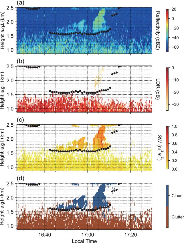
1746                                                   X. Hu et al.: A robust low-level cloud and clutter discrimination method

Figure 2. (a) Raw reflectivity and (c) noise-removed reflectivity from 12:08 to 12:29 LT on 28 May 2014. (b) The 300 reflectivity profiles of
the same duration; the dashed blue line is noise-equivalent reflectivity curve.

ity if the velocity difference is positive (or negative) (John-          2.8 km has relatively higher LDRs than the precipitation be-
son et al., 2017; Sokol et al., 2018). The adjusted velocity is          low and the ice particles above. Clutter near the surface be-
shown in Fig. 3c, where the upwards velocity at the lower                fore the precipitation reaches the surface at about 20:30 LT
level of atmosphere is de-aliased to downwards (smooth blue              has similar high LDR values. Clutter layer can appear as
region in Fig. 3c and orange dots in Fig. 3d). The de-aliased            high as 3 km a.g.l. during daytime in the warm season at the
velocity and reflectivity are then averaged over 1 min to re-            SACOL site, which is close to or even higher than melt-
duce the effect of wind drift. These range bins with averaged            ing layer height. In order to avoid wrongly identifying the
reflectivity greater than 10 dBZ and averaged velocity lower             melting layer with high LDR as clutter, the melting layer
than −3 m s−1 are identified as precipitation (Chandra et al.,           is recognized by analyzing the gradient of reflectivity and
2015). However, the drizzle with smaller sizes and lower ve-             velocity that has a large value associated with the melting
locity (Kollias et al., 2011; O’Connor et al., 2005) may not be          layer (Baldini and Gorgucci, 2006; Matrosov et al., 2007;
identified by the above method. Thus, the radar echoes that              Perry et al., 2017). The peak of |reflectivity0 | × |velocity0 |
below the lidar-detected cloud base, while still being con-              (Fig. 4e) is located as the middle of the melting layer for each
nected to the cloud, are marked as drizzle (Wu et al., 2015;             identified precipitation profile; then the height of maximum
Yang et al., 2018) and removed from the training data.                   (|reflectivity0 | × |velocity0 |)00 up to 500 m above (below) the
   Water-coated ice particles inside the melting layer are               peak is defined as the top (bottom) of melting layer as shown
largely non-spherical; therefore, they have high LDR val-                in Fig. 4e with red dots (Devisetty et al., 2019; Khanal et al.,
ues, similar to insects (Brandes and Ikeda, 2004; Islam et al.,          2019). The identified melting layer and precipitation are plot-
2012). This can be seen in Fig. 4c. The melting layer around             ted in Fig. 4a–c as black dots and the slashed shading area.

Atmos. Meas. Tech., 14, 1743–1759, 2021                                                    https://doi.org/10.5194/amt-14-1743-2021
X. Hu et al.: A robust low-level cloud and clutter discrimination method                                                            1747

Figure 3. (a) Reflectivity, (b) radar-measured Doppler velocity, and (c) de-aliased velocity from 18:56 to 19:10 LT on 30 August 2013. (d)
Raw and de-aliased velocity profile of the dashed white line in the left panels; the dashed gray line is the maximum unambiguous velocity
(±10.38 m s−1 for SACOL KAZR). Positive velocity represents upwards velocity.

3.2   Creating multi-dimensional PDFs                                  monly higher in the warm seasons when they swarm (Abrol,
                                                                       2015). The seasonal dependence of radar reflectivity is con-
To capture the differences between clouds and clutter as ac-           sidered as a factor to build the PDFs. Clutter also generally
curately as possible, we need to choose the appropriate dis-           has lower SW and lower vertical velocity because insects
criminants before creating the PDFs for both. From a statis-           may actively oppose environmental vertical motion and con-
tical point of view, the description of differences in higher-         trol their own flying behavior, while cloud particles are more
dimensional space is generally more complete than in lower-            vulnerable to small-scale local turbulence and entrainment
dimensional space. Increasing the number of discriminants              processes (Geerts and Miao, 2005). Yet after checking both
could decrease the overlapping region of the two PDFs,                 variables, we found that distributions of SW for clouds and
thereby reducing the fraction of ambiguous classifications             clutter are more discrepant than that of vertical velocity; thus,
(Liu et al., 2004). However, only when the added discrimi-             SW is used to build the PDFs rather than using vertical ve-
nant is largely independent of the other used, can it improve          locity directly. One distinctive characteristic of insects that
the classification significantly (Liu et al., 2009). After care-       differs from other fixed clutter is that their behavior is influ-
fully examining all radar variables for many specific clut-            enced by many natural factors (Chapman et al., 2015; John-
ter and cloud cases, we chose radar reflectivity, LDR, and             son et al., 2016; Thomas et al., 2003). For example, insects’
SW along with their time–height and seasonal dependence                number density has a high correlation with surface tempera-
as discriminants. LDR is chosen because it has distinct dis-           ture (Luke et al., 2008); thus, the maximum height and radar
tributions for clouds and clutter due to their shape difference        echo intensity of insects have strong diurnal cycles (Hubbert
(cloud droplets are largely spherical, while clutter is non-           et al., 2018; Wood et al., 2009). The time and height varia-
spherical). Insects’ number density and sizes make them of-            tions of radar echoes are thereby considered in the construc-
ten generate low radar reflectivity, which has a similar range         tion of multi-dimensional PDFs.
with strati and broken cumuli (Luke et al., 2008) but is com-

https://doi.org/10.5194/amt-14-1743-2021                                                  Atmos. Meas. Tech., 14, 1743–1759, 2021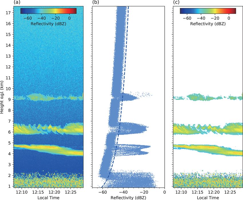
1748 X. Hu et al.: A robust low-level cloud and clutter discrimination method
Figure 4. (a) Reflectivity, (b) velocity, and (c) LDR from 20:15 to 20:45 LT on 10 August 2013. (d) Reflectivity and velocity, and (e)
|reflectivity0 | × |velocity0 | profile of the dashed white line in panels (a–b). Black dots and the slashed shading area in panels (a–c) are the
identified melting layer and precipitation. Red dots in panel (e) are the identified bottom and top of the melting layer.
Once the discriminant factors are selected, the cloud and trasting distributions during the cold season. Nevertheless,
clutter samples need to be extracted for building the multi- both clouds and clutter occur less frequently compared to the
dimensional PDFs. The radar echoes above the lidar cloud warm season (Zhu et al., 2017). Note that some overlapping
base height after removing noise and non-cloud meteorolog- regions of cloud and clutter PDFs still occur (e.g., Fig. 5b3).
ical targets are considered to be clouds; otherwise, they are However, the multi-dimensional PDFs made the ambiguity
clutter. Based on the lidar auxiliary data, all the radar echoes area much smaller compared with the results by only using a
below 3.6 km from August 2014 to July 2015 are separated single discriminant. The significant differences between clut-
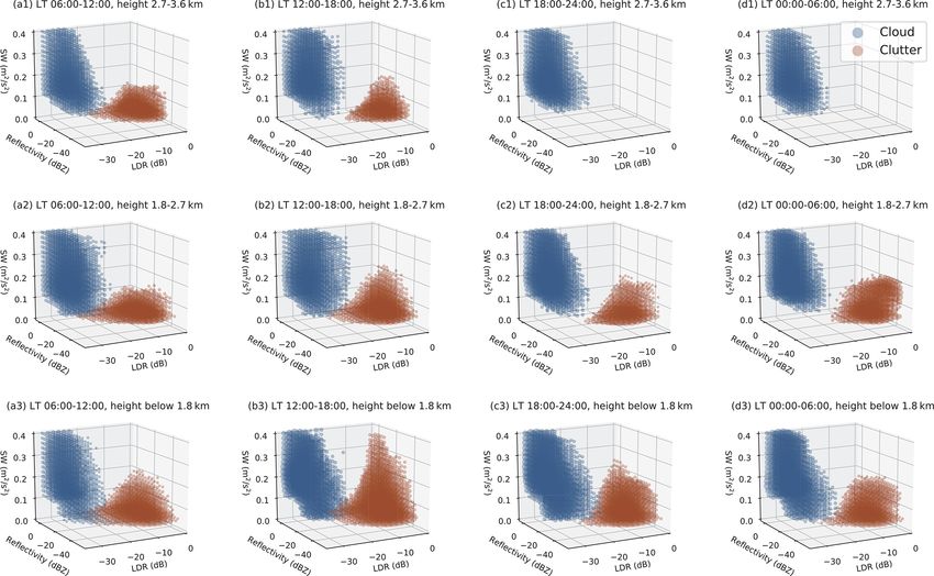
into cloud or clutter samples. Figures 5 and 6 show the multi- ter and cloud PDFs (Figs. 5 and 6) can be used to adequately
dimensional PDFs for different local times and heights for separate them more accurately.
the warm and cold seasons, respectively, which is calculated
as the number of samples in each discriminant range for each 3.3 Generating classification mask based on Bayesian
class (clouds or clutter), divided by the total number of sam- method
ples in each discriminant range for all classes. After exam-
ining 1-year data, it is found that 3.6 km a.g.l. is the highest The obtained multi-dimensional PDFs are then used to train
level that clutter can reach at the SACOL site. As expected, the optimal Bayesian classifier to separate clouds and clutter
clutter tends to have lower reflectivity (lower density), larger for any observed discriminants (XO ). According to Bayesian
LDR (non-spherical shape) and lower SW (less turbulent mo- method, the probability of a radar range gate with dis-
tion) compared with clouds (Figs. 5 and 6). Insect activities criminants X = XO = ReflectivityO , LDRO , SWO , timeO ,
are largely influenced by temperature; thus, the clutter ap- heightO , seasonO being class Ci , (i ∈ [cloud, clutter]) can be
pears mostly during daytime and its height has an obvious estimated as
diurnal cycle. It is also notable that there is no clutter above
2.7 km during nighttime (Figs. 5c1, d1 and 6c1, d1). The
p X = XO |Ci p (Ci )
three radar variables for clouds and clutter still have con- p Ci |X = X O
= , (1)
p X = XO
Atmos. Meas. Tech., 14, 1743–1759, 2021 https://doi.org/10.5194/amt-14-1743-2021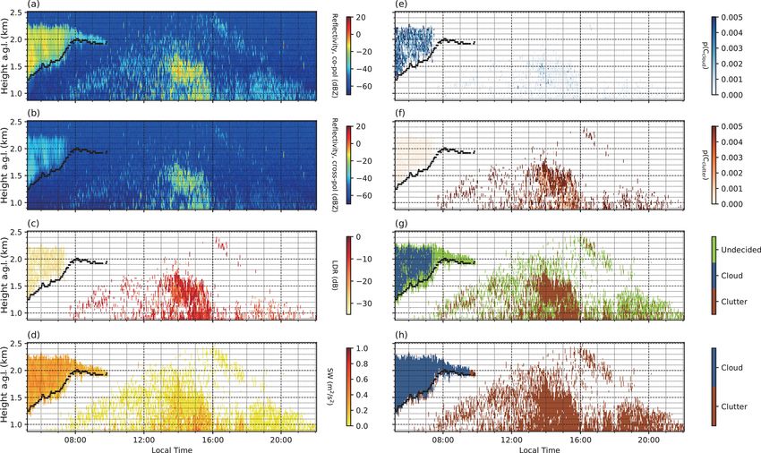
X. Hu et al.: A robust low-level cloud and clutter discrimination method                                                          1749

Figure 5. The multi-dimensional PDFs of clutter (brown dots) and cloud droplets (blue dots) at 06:00–12:00 (column a), 12:00–18:00
(column b), 18:00–24:00 (column c), and 00:00–06:00 LT (column d), and height below 1.8 km (row 3), 1.8–2.7 km (row 2) and 2.7–3.6 km
(row 1) in the warm season (April to September). The size of dots represents the value of probability density.

where the priori probabilities are assumed to be equal               3.4   Applying a low-pass spatial filter to undecided
for all classes (Golbon-Haghighi et al., 2016; Ma et al.,                  mask
2019), which means p(Ccloud ) = p(Cclutter ) = 1/2. Further-
more, p(X = XO ) is the same for all classes; hence, Eq. (1)
can be rewritten as                                                  The Bayesian classifier is able to separate clouds and clutter
                                                                     in most cases when all the radar discriminants as described in

p Ci |X = XO = Kp X = XO |Ci ,                           (2)         Sect. 3.2 and 3.3 are offered. Figure 7 shows such a case from
                                                                     05:00 to 22:00 LT on 24 September 2013. Unsurprisingly,
                                                                     these radar range bins with low reflectivity (Fig. 7a), high
where K is constant for all classes                                  LDR (Fig. 7c), and low SW (Fig. 7d) are considered more
                                                                     likely to be clutter rather than clouds (Fig. 7e, f and g), while
            1
K=                 ,                                       (3)      high reflectivity, low LDR, and high SW have higher prob-
     2p X = XO                                                       ability to be clouds (Fig. 7a–g). When the individual three
                                                                     radar variables disagree on the classification, for example,
and p(X = XO |Ci ) is the conditional probability of discrim-        this clutter from 12:00 to 16:00 LT near the surface with high
inants being XO for each class, which has been derived from          reflectivity and high SW (likely to be clouds) and high LDR
1-year training data as described in Sect. 3.2.                      (also likely to be clutter), the Bayesian classifier can still cor-
   For any given observation of discriminants, the posterior         rectly separate them, as shown in Fig. 7g. However, the cloud
probability for each class p(Ci |X = XO ) is estimated ac-           radar may not always provide valid observations. For exam-
cordingly and compared to decide its category. The radar             ple, LDR can only be computed when both co- and cross-
range gate belongs to clouds only when p(Ccloud |X =                 polarized reflectivities are available. Figure 7a and b show
XO ) is larger than p(Cclutter |X = XO ). And vice versa, if         the reflectivities of co- and the cross-polarized channels, re-
p(Cclutter |X = X O ) is larger than p(Ccloud |X = XO ), it is       spectively. There are some range gates where co-polarized
considered to be a clutter gate.                                     reflectivity detects signal (cloud or clutter), while no signal

https://doi.org/10.5194/amt-14-1743-2021                                                Atmos. Meas. Tech., 14, 1743–1759, 2021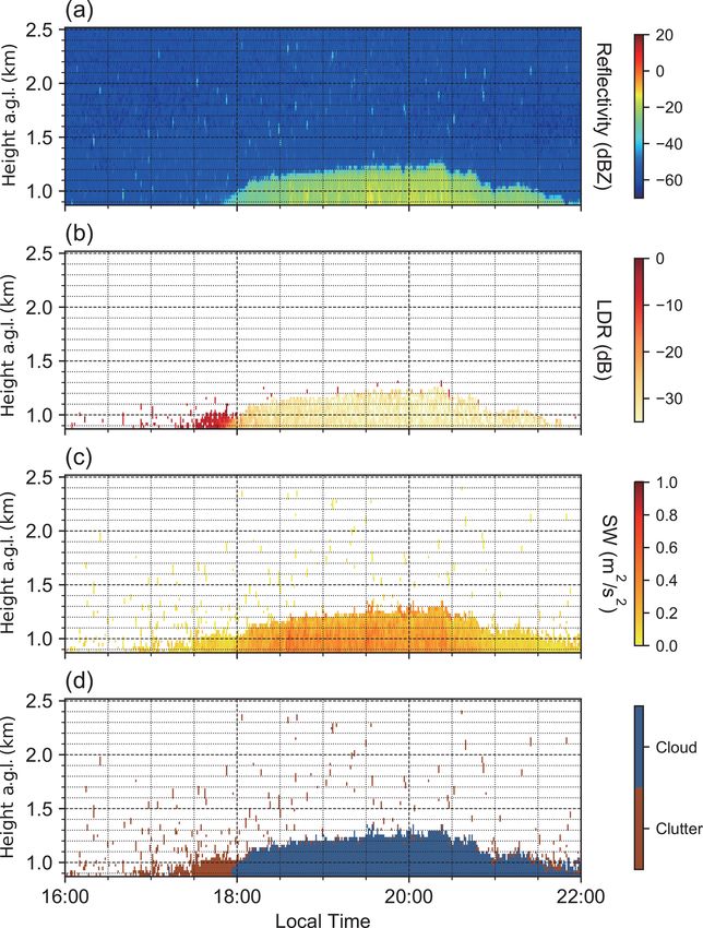
1750 X. Hu et al.: A robust low-level cloud and clutter discrimination method
Figure 6. Same as Fig. 5 but for the cold season (October to March).
is detected in the cross-polarized channel, which causes the nal classification mask result is shown in Fig. 7h. Comparing
missing LDR in these radar range gates (e.g., the rightmost with lidar observation on the same day, the undecided range
range bins above the lidar cloud base and some bins scat- bins are correctly categorized into clutter (green dots turned
tering near-surface in Fig. 7c). Without the LDR input data, to brown) and clouds (green dots turned to blue above li-
the Bayesian classifier fails to work (green dots in Fig. 7g), dar cloud base) after applying the low-pass spatial filter. It is
because no conditional probability was established for an in- clear from Fig. 7h that clutter layer height has an apparent di-
complete XO . Mathematically, there are several approaches urnal cycle and the insects’ number density is much stronger
to deal with missing data for the Bayesian method, such as in the early afternoon near the surface (patchy high reflectiv-
assuming a distribution of them (Linero and Daniels, 2018). ity rather than dotted low reflectivity). This is why time and
However, in practice, we find it is uneconomical to solve height are also chosen as the discriminants.
such an issue. Rather, we utilize the spatial correlation differ-
ence between clouds and clutter to process the Bayesian un-
decided classifications, which is more effective and simpler. 4 Result
As mentioned earlier, cloud droplets are highly correlated in
time and space, while clutter does not have the same feature. 4.1 Case study
For those radar bins that cannot be identified as clouds or
clutter from the probability estimate, we use their neighbor- We apply the identification algorithm to a whole year of
ing range gates to provide information to help make the final radar data to discriminate low-level clouds and clutter. The
decision. A spatial filter with five range bins respecting to results are compared with the simultaneous lidar cloud base
height (150 m) and five range bins concerning time (21.4 s), to demonstrate the performance of the algorithm.
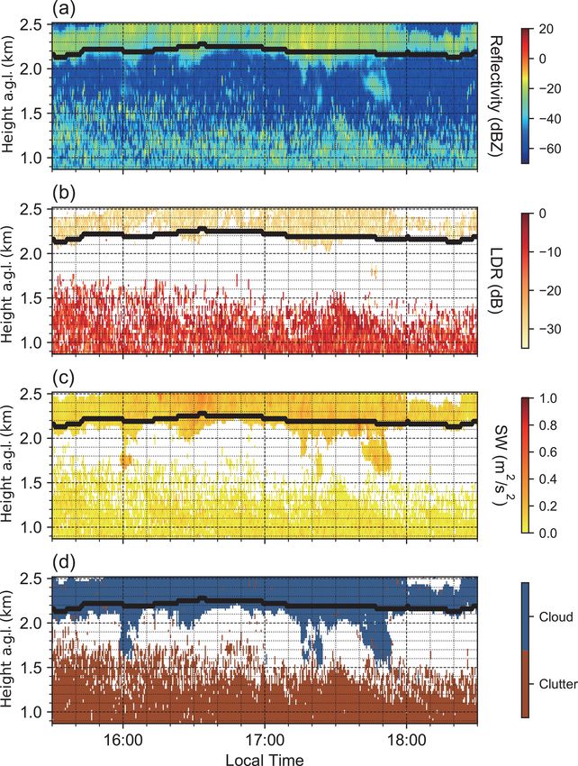
which is centered at each undecided classification bin, is em- Figure 8 shows a case of broken cumulus from 16:27 to
ployed here (Hu et al., 2020; Marchand et al., 2008). Fol- 17:30 LT on 15 April 2014. During this period, a substan-
lowing Ge et al. (2017), if the number of cloud range bins tial presence of insects is observed below the broken cu-
in the box is less than 13, this range bin is considered to be mulus. The top of the insect layer is around 1.6 km, where
clutter; otherwise, it will be marked as a cloud bin. The fi- there is also the cloud base height detected by lidar and
our algorithm (Fig. 8d). From the radar reflectivity image in
Atmos. Meas. Tech., 14, 1743–1759, 2021 https://doi.org/10.5194/amt-14-1743-2021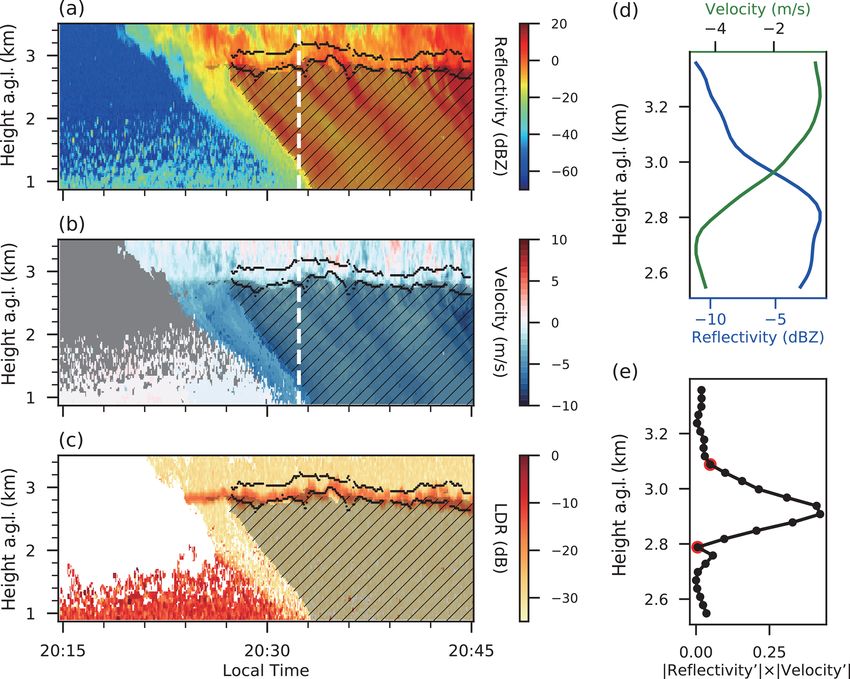
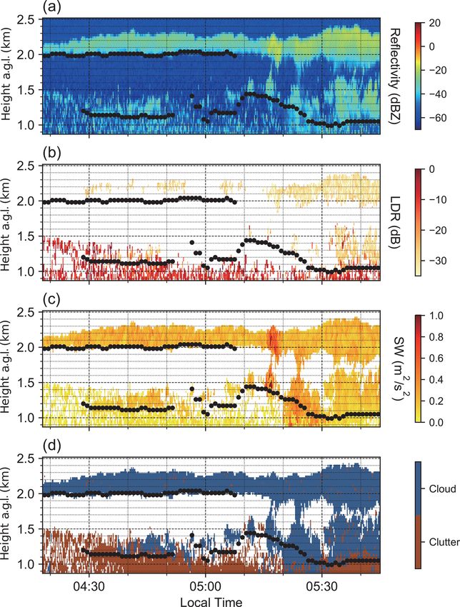
X. Hu et al.: A robust low-level cloud and clutter discrimination method                                                                  1751

Figure 7. (a) Reflectivity of co-polarized (co-pol), (b) reflectivity of cross-polarized (cross-pol), (c) LDR, (d) SW, (e) estimated probability
of cloud, (f) estimated probability of clutter, (g) classification mask using the Bayesian method, and (h) classification mask after the spatial
filter from 05:00 to 22:00 LT on 24 September 2013. The black dots represent lidar-detected cloud base height.

Fig. 8a, the cloud droplets begin to dissipate due to entrain-               Figure 10 shows a case of precipitating stratocumulus.
ment (Chernykh et al., 2001; Pinsky and Khain, 2019) and                  The drizzle droplets that fall from the cloud base are kept
have similar reflectivity values as clutter (around −50 dBZ)              as clouds (Fig. 10d), since they have relatively small falling
around the cloud base. As shown in Fig. 8b, clutter has the               velocity and reflectivity, and cannot be recognized as pre-
LDRs mostly greater than −15 dB but clouds have relatively                cipitation by the algorithm. The edges between clutter and
smaller LDR values. The high SW above the cloud base                      drizzle are blurry in radar reflectivity and SW (Fig. 10a and
(more than 0.4 m2 s−2 ) indicates strong turbulence inside the            c). Under this circumstance, the algorithm identifies the clut-
cumulus. Combining all these radar variables together, our                ter near the surface with large LDR (larger than −15 dB) but
clutter identification algorithm shows a great agreement with             keeps the drizzle as hydrometeors with a low-pass filter since
lidar detection (Fig. 8d).                                                they are temporally and spatially correlated (Fig. 10b). Note
   Figure 9 shows a case of stratus clouds embedded in insect             that although the bottom of identified hydrometeors is coin-
layers. The reflectivity inside clouds is similar to the clut-            cidental with the top height of the clutter layer (Fig. 10d), it
ter reflectivity (between −40 to −20 dBZ) but is distributed              does not mean that the drizzle droplets “suddenly” all evap-
more homogeneously in time and space (Fig. 9a). Note that                 orate when they fall into the insect layer. The drizzle may
for these flat clouds, Kalapureddy et al. (2018) used the stan-           still fall toward the ground; however, the signals are much
dard deviation of reflectivity to remove clutter. However,                smaller than that from the insect layer. In other words, the
this method causes some false positives (clouds are wrongly               clutter mask does not necessarily mean only clutter can be
identified as clutter) around fuzzy cloud edges. The stratus              in this range bin; rather, the backscattered power is largely
cloud is typically more featureless than the cumulus (Fig. 8)             dominated by insects.
due to the absence of active convective elements (Harrison                   Figure 11 shows a case of broken cumulus and shallow
et al., 2017), and it has lower SW values which may fall                  convective clouds under stratus. One can see a few thin
within the same range as clutter (below 0.4 m2 s−2 ; Fig. 9c).            clouds (less than 300 m) below 1.5 km a.g.l. during 04:55 to
Thus, in this case, the LDR (Fig. 9b) and spatial filter in our           05:15 LT and some broken cumulus from 04:30 to 04:50 LT
method made the major contribution to separate them.                      like the case shown in Fig. 8 but with lower cloud top and

https://doi.org/10.5194/amt-14-1743-2021                                                      Atmos. Meas. Tech., 14, 1743–1759, 2021
1752                                                  X. Hu et al.: A robust low-level cloud and clutter discrimination method

Figure 8. (a) Reflectivity, (b) LDR, (c) SW, and (d) classification   Figure 9. Same as Fig. 8 but for 09:25 to 10:25 LT on 12 October
mask from 16:27 to 17:31 LT on 15 April 2014. The black dots are      2013.
lidar-detected cloud base.

                                                                      We believe the identified cloud masks below lidar cloud base
base heights (“more deeply buried” in the clutter layer).             from 05:15 to 05:30 LT are drizzle particles because of the
There may be many insets in the cloud, causing the large              virga reflectivity during that time (Fig. 11a).
radar-observed LDR, e.g., from 04:30 to 04:40 LT (greater                Figure 12 shows a case of low-level clouds completely sur-
than −15 dB; Fig. 11b); therefore, these range gates are clas-        rounded by intense insects. This is the most difficult case
sified as clutter by our algorithm (Fig. 11d). The clouds,            to discriminate, because cloud signals are heavily contami-
which are less affected by insects from 04:40 to 04:50 LT             nated by clutter. Figure 12d shows that the identified cloud
(lower LDR than −15 dB and higher SW than 0.4 m2 s−2 ),               masks correspond well with lidar cloud base during 14:15 to
are identified as clouds without doubt. Note the occurrence of        16:00 LT, due to lower LDR (less than −15 dB; Fig. 12b)
interlaced blocky appearance of classification masks around           and higher SW (greater than 0.4 m2 s−2 ; Fig. 12c) of the
04:40 LT (Fig. 11d). There are only few available LDR                 cloud particles. However, the algorithm misses some clouds
range gates there (Fig. 11b), meaning the classification masks        with low SW (around 0.2 m2 s−2 ; Fig. 12c) from 16:00 to
are mostly achieved by the spatial filter (Sect. 3.4), which          16:40 LT. Note that a large number of LDRs are unavailable
causes some misclassification (e.g., from 04:30 to 04:40 LT)          for this cloud (Fig. 12b) and its structure is loose (Fig. 12a),
because the spatial correlation of clouds is reduced since            especially around cloud edges where clutter signals are even
they are largely contaminated by clutter. During 04:55 to             stronger than clouds. In this circumstance, the algorithm can
05:15 LT, a few broken clouds higher away from the clut-              only identify a part of the cloud.
ter layer are successfully identified by the algorithm, which            Figure 13 shows a case of shallow cumulus near the sur-
is in accordance with the MPL lidar detection, indicating the         face in the cold season. Compared with the earlier cases
spatial filter does work well when clouds are not adjacent to         (Figs. 8–12), the clutter in this case is less organized. There
falsely identified masks. The shallow convective clouds af-           is no dense insect layer gathering near the surface. The dif-
ter 05:15 LT are more turbulent (SW greater than 0.6 m2 s−2 ;         ferent behavior of insects in the warm and cold seasons is
Fig. 11c) than these broken cumuli; thus, they are effectively        why seasonal variation is chosen as a discriminant. The radar
identified as clouds even with a dense clutter layer below.           reflectivity in the cumulus is more homogenous than that

Atmos. Meas. Tech., 14, 1743–1759, 2021                                                https://doi.org/10.5194/amt-14-1743-2021
X. Hu et al.: A robust low-level cloud and clutter discrimination method 1753
Figure 10. Same as Fig. 8 but from 15:30 to 18:30 LT on 7 July Figure 11. Same as Fig. 8 but for 04:18 to 05:45 LT on 20 July
2014. 2014.
from the scattering clutter (Fig. 13a) and can easily be identi- dated by lidar detection (“true” or “false” clutter classifica-
fied even through human eyes. Shallow cumulus clouds have tion mask). Note that the evaluation is focused on the identi-
LDR of less than −20 dB, whereas clutter has higher LDR fied clutter rather than low-level clouds, because lidar power
greater than −15 dB (Fig. 13b). Higher SW values (around is often attenuated by optically thick low-level water clouds,
0.6 m2 s−2 ; Fig. 13c) in the cumulus during 18:00 to 20:30 LT leading to a significant discrepancy between radar- and lidar-
indicate that the cloud droplets are more affected by small- measured low-level clouds, while the “true” or “false” clutter
scale local turbulence and entrainment processes. The algo- only relies on lidar cloud base height, which would cause less
rithm can screen out the shallow cumulus in the cold season uncertainty in the assessment.
and filter out the clutter (Fig. 13e). Figure 14 illustrates the PD and PFA as functions of reflec-
tivity (a), LDR (b), SW (c), time (d), and height (e). The PD
4.2 The 1-year evaluation
(solid lines) is usually above 98 %, except when reflectivity
To further objectively demonstrate the performance of this is larger than −10 dBZ (Fig. 14a), LDR lower than −15 dB
algorithm, probability of detection (PD ) and false alarm rate (Fig. 14b), or SW larger than 0.2 m2 s−2 (Fig. 14c), where
(PFA ) are calculated using 1-year data (August 2013 to July clutter has similar properties to clouds, however, which are
2014) that are defined as only small portions of the whole dataset, as shown in Figs. 5
and 6. So the seasonally and yearly averaged PD values are
TP all near or above 98 % (Fig. 14f). Similarly, for the cloud with
PD = reflectivity lower than −30 dBZ (Fig. 14a), LDR larger than
TP + FN
FP −20 dB (Fig. 14b), and SW lower than 0.1 m2 s−2 (Fig. 14c),
PFA = , (4) there are chances that clouds are falsely identified as clut-
FP + TN
ter (higher PFA , dashed lines). The PFA values are below
where the number of TP (true positives), TN (true negatives), 0.5 % in all seasons (Fig. 14f). Using a single LDR thresh-
FP (false positives) and FN (false negatives) is based on our old to filter out clutter would induce a sharp increase of
algorithm-identified clutter (“positive” of “negative”) vali- PD from 0 % to 100 % at the threshold point. Very differ-
https://doi.org/10.5194/amt-14-1743-2021 Atmos. Meas. Tech., 14, 1743–1759, 20211754 X. Hu et al.: A robust low-level cloud and clutter discrimination method
Figure 12. Same as Fig. 8 but for 14:15 to 17:00 LT on 19 August Figure 13. Same as Fig. 8 but for 16:00 to 22:00 LT on 4 February
2013. 2014. Note that the lidar observation is missed that day.
ent from that, by using multi-dimensional PDFs with the tial filter is applied to the Bayesian undecided classification
Bayesian method, it can correctly identify cloud-like clut- mask, considering the spatial correlation difference between
ter and clutter-like cloud; thus, they increase the accuracy of clouds and clutter. The case studies indicate the algorithm
the classification mask. Both PD and PFA are less fluctuat- can filter out most of the clutter while still maintaining the
ing with time (Fig. 14d) and height (Fig. 14e) compared with low-level clouds (including drizzle), even when they are em-
the three radar variables (Fig. 14a–c), except for PD above bedded in clutter layer. Unlike the traditional way of select-
3.2 km, where the clutter is extremely rare (fewer samples). ing a single LDR threshold to remove the clutter, this al-
This indicates that the time and height variations of cloud and gorithm particularly shows higher accuracy for clutter-like
clutter features are well captured by the multi-dimensional clouds or cloud-like clutter. The 1-year evaluation demon-
PDFs. The PD and PFA of the whole year (black lines) are strates the good performance of this algorithm (98.5 % de-
more consistent with that of warm season (red line), because tection rate and 0.4 % false alarm rate). For the quantitative
clutter more frequently appears in the warm season. Overall, evaluation, the lidar-detected cloud base is assumed to be
the 1-year evaluation shows that the algorithm can success- perfectly correct, and the small temporal and spatial offsets
fully filter clutter out with a high value of PD (98.45 %) and between the radar and lidar are assumed to have a small im-
a very low value of PFA (0.37 %), as shown in Fig. 14f. pact. We conclude that this algorithm satisfactorily retains
low-level clouds and removes radar clutter at the SACOL
site.
5 Summary and discussion For the non-cloud low-level meteorological target, such as
precipitation and melting layer, we use radar observation it-
We develop a low-level cloud and clutter discrimination al- self to identify them (Chandra et al., 2015; Matrosov et al.,
gorithm for a ground-based cloud radar based on multi- 2007). Although it might not be as reliable as the method
dimensional PDFs with the Bayesian method using cloud by combining the radar with other instruments such as rain
radar reflectivity, LDR, SW, and their time of the day, height, gauge, it would still be enough to effectively reduce the mis-
and season dependence as discriminants. A low-pass spa- classification of clutter and clouds. The more accurate esti-
Atmos. Meas. Tech., 14, 1743–1759, 2021 https://doi.org/10.5194/amt-14-1743-2021X. Hu et al.: A robust low-level cloud and clutter discrimination method 1755
Figure 14. Probability of detection (PD , solid line) and false alarm rate (PFA , dashed line) as function of reflectivity (a), LDR (b), SW (c),
time (d), and height (e) for the warm season (red line), cold season (blue line), and whole year (black line). The values of PD and PFA for
the warm season, cold season, and whole year are shown in panel (f).
mation of rain rate will be carried out in our future work, editor, and Andreas Richter, the handling executive editor, for all
along with this algorithm, used to provide more reliable low- the support.
level cloud and precipitation radar data to study its climate
effect and the interaction with local abundant dust aerosol in
semi-arid regions. Financial support. This research has been supported by the
National Science Foundation of China (grant nos. 41922032,
41875028, and 91937302) and the National Key R & D Program
Data availability. Both the lidar and radar data used in this study of China (grant no. 2016YFC0401003).
can be acquired from the SACOL site (http://climate.lzu.edu.cn)
(SACOL, 2021).
Review statement. This paper was edited by Brian Kahn and re-
viewed by three anonymous referees.
Author contributions. XH and JG designed the study. XH, JD, and
QL performed the cloud and clutter discrimination. JH and QF
discussed the method and the results. XH and JG prepared the
References
manuscript with significant contributions from all co-authors.
Abrol, D. P.: Diversity of pollinating insects visiting litchi
flowers (Litchi chinensis Sonn.) and path analysis of en-
Competing interests. The authors declare that they have no conflict vironmental factors influencing foraging behaviour of
of interest. four honeybee species, J. Apicult. Res., 45, 180–187,
https://doi.org/10.1080/00218839.2006.11101345, 2015.
Arulraj, M. and Barros, A. P.: Shallow Precipitation Detection
Acknowledgements. The authors would like to thank the SACOL and Classification Using Multifrequency Radar Observations and
team (http://climate.lzu.edu.cn, last access: 23 February 2021) for Model Simulations, J. Atmos. Ocean. Tech., 34, 1963–1983,
supporting the radar and lidar data. The authors would like to thank https://doi.org/10.1175/jtech-d-17-0060.1, 2017.
the three anonymous referees for the constructive comments. The Bala, G., Caldeira, K., Nemani, R., Cao, L., Ban-Weiss, G., and
authors would also like to thank Brian Kahn, the handling associate Shin, H.-J.: Albedo enhancement of marine clouds to counteract
global warming: impacts on the hydrological cycle, Clim. Dy-
https://doi.org/10.5194/amt-14-1743-2021 Atmos. Meas. Tech., 14, 1743–1759, 20211756 X. Hu et al.: A robust low-level cloud and clutter discrimination method
nam., 37, 915–931, https://doi.org/10.1007/s00382-010-0868-1, Layer Temperatures, Atmosphere-Basel, 9, 377,
2010. https://doi.org/10.3390/atmos9100377, 2018.
Baldini, L. and Gorgucci, E.: Identification of the Melt- Garrett, T. J. and Zhao, C.: Ground-based remote sensing of
ing Layer through Dual-Polarization Radar Measurements at thin clouds in the Arctic, Atmos. Meas. Tech., 6, 1227–1243,
Vertical Incidence, J. Atmos. Ocean. Tech., 23, 829–839, https://doi.org/10.5194/amt-6-1227-2013, 2013.
https://doi.org/10.1175/jtech1884.1, 2006. Ge, J., Zhu, Z., Zheng, C., Xie, H., Zhou, T., Huang, J., and Fu, Q.:
Bony, S., Stevens, B., Frierson, D. M. W., Jakob, C., Kageyama, M., An improved hydrometeor detection method for millimeter-
Pincus, R., Shepherd, T. G., Sherwood, S. C., Siebesma, A. P., wavelength cloud radar, Atmos. Chem. Phys., 17, 9035–9047,
Sobel, A. H., Watanabe, M., and Webb, M. J.: Clouds, cir- https://doi.org/10.5194/acp-17-9035-2017, 2017.
culation and climate sensitivity, Nat. Geosci., 8, 261–268, Ge, J., Zheng, C., Xie, H., Xin, Y., Huang, J., and Fu, Q.: Midlati-
https://doi.org/10.1038/ngeo2398, 2015. tude Cirrus Clouds at the SACOL Site: Macrophysical Properties
Brandes, E. A. and Ikeda, K.: Freezing-Level Estimation and Large-Scale Atmospheric States, J. Geophys. Res.-Atmos.,
with Polarimetric Radar, J. Appl. Meteorol., 43, 1541–1553, 123, 2256–2271, https://doi.org/10.1002/2017jd027724, 2018.
https://doi.org/10.1175/jam2155.1, 2004. Ge, J., Wang, Z., Liu, Y., Su, J., Wang, C., and Dong, Z.: Link-
Brient, F. and Bony, S.: Interpretation of the positive low-cloud ages between mid-latitude cirrus cloud properties and large-scale
feedback predicted by a climate model under global warming, meteorology at the SACOL site, Clim. Dynam., 53, 5035–5046,
Clim. Dynam., 40, 2415–2431, https://doi.org/10.1007/s00382- https://doi.org/10.1007/s00382-019-04843-9, 2019.
011-1279-7, 2012. Ge, J. M., Huang, J. P., Xu, C. P., Qi, Y. L., and Liu, H. Y.: Charac-
Ceppi, P., Hartmann, D. L., and Webb, M. J.: Mechanisms of the teristics of Taklimakan dust emission and distribution: A satellite
Negative Shortwave Cloud Feedback in Middle to High Lati- and reanalysis field perspective, J. Geophys. Res.-Atmos., 119,
tudes, J. Climate, 29, 139–157, https://doi.org/10.1175/jcli-d-15- 11772–11783, https://doi.org/10.1002/2014jd022280, 2014.
0327.1, 2016. Geerts, B. and Miao, Q.: The Use of Millimeter Doppler Radar
Chandra, A., Zhang, C., Kollias, P., Matrosov, S., and Szyrmer, W.: Echoes to Estimate Vertical Air Velocities in the Fair-Weather
Automated rain rate estimates using the Ka-band ARM Convective Boundary Layer, J. Atmos. Ocean. Tech., 22, 225–
zenith radar (KAZR), Atmos. Meas. Tech., 8, 3685–3699, 246, https://doi.org/10.1175/jtech1699.1, 2005.
https://doi.org/10.5194/amt-8-3685-2015, 2015. Givati, A. and Rosenfeld, D.: Quantifying Precipita-
Chapman, J. W., Reynolds, D. R., Wilson, K., and Holyoak, M.: tion Suppression Due to Air Pollution, J. Appl. Me-
Long-range seasonal migration in insects: mechanisms, evolu- teorol., 43, 1038–1056, https://doi.org/10.1175/1520-
tionary drivers and ecological consequences, Ecol. Lett., 18, 0450(2004)0432.0.Co;2, 2004.
287–302, https://doi.org/10.1111/ele.12407, 2015. Golbon-Haghighi, M.-H., Zhang, G., Li, Y., and Doviak, R.:
Chernykh, I. V., Alduchov, O. A., and Eskridge, R. E.: Detection of Ground Clutter from Weather Radar Using a
Trends in Low and High Cloud Boundaries and Errors Dual-Polarization and Dual-Scan Method, Atmosphere, 7, 83,
in Height Determination of Cloud Boundaries, B. Am. https://doi.org/10.3390/atmos7060083, 2016.
Meteorol. Soc., 82, 1941–1947, https://doi.org/10.1175/1520- Görsdorf, U., Lehmann, V., Bauer-Pfundstein, M., Peters, G.,
0477(2001)0822.3.Co;2, 2001. Vavriv, D., Vinogradov, V., and Volkov, V.: A 35-GHz Polari-
Clothiaux, E. E., Ackerman, T. P., Mace, G. G., Moran, K. P., Marc- metric Doppler Radar for Long-Term Observations of Cloud Pa-
hand, R. T., Miller, M. A., and Martner, B. E.: Objective De- rameters – Description of System and Data Processing, J. At-
termination of Cloud Heights and Radar Reflectivities Using a mos. Ocean. Tech., 32, 675–690, https://doi.org/10.1175/jtech-
Combination of Active Remote Sensors at the ARM CART Sites, d-14-00066.1, 2015.
J. Appl. Meteorol., 39, 645–665, https://doi.org/10.1175/1520- Harrison, R. G., Nicoll, K. A., and Aplin, K. L.: Evaluating strati-
0450(2000)0392.0.co;2, 2000. form cloud base charge remotely, Geophys. Res. Lett., 44, 6407–
Devisetty, H. K., Jha, A. K., Das, S. K., Deshpande, S. M., Kr- 6412, https://doi.org/10.1002/2017gl073128, 2017.
ishna, U. V. M., Kalekar, P. M., and Pandithurai, G.: A case study Hu, X., Ge, J., Li, Y., Marchand, R., Huang, J., and
on bright band transition from very light to heavy rain using si- Fu, Q.: Improved Hydrometeor Detection Method: An Ap-
multaneous observations of collocated X- and Ka-band radars, J. plication to CloudSat, Earth Space Sci., 7, e2019EA000900,
Earth Syst. Sci., 128, 136, https://doi.org/10.1007/s12040-019- https://doi.org/10.1029/2019ea000900, 2020.
1171-0, 2019. Huang, J., Ge, J., and Weng, F.: Detection of Asia dust storms using
Fu, Q. and Feng, S.: Responses of terrestrial aridity to multisensor satellite measurements, Remote Sens. Environ., 110,
global warming, J. Geophys. Res.-Atmos., 119, 7863–7875, 186–191, https://doi.org/10.1016/j.rse.2007.02.022, 2007.
https://doi.org/10.1002/2014jd021608, 2014. Huang, J., Huang, Z., Bi, J., Zhang, W., and Zhang, L.:
Fu, Q., Carlin, B., and Mace, G.: Cirrus horizontal inhomo- Micro-Pulse Lidar Measurements of Aerosol Vertical Struc-
geneity and OLR bias, Geophys. Res. Lett., 27, 3341–3344, ture over the Loess Plateau, Atmos. Ocean. Sci. Lett., 1, 8–11,
https://doi.org/10.1029/2000gl011944, 2000. https://doi.org/10.1080/16742834.2008.11446756, 2008a.
Fu, Q., Baker, M., and Hartmann, D. L.: Tropical cirrus and water Huang, J., Zhang, W., Zuo, J., Bi, J., Shi, J., Wang, X., Chang, Z.,
vapor: an effective Earth infrared iris feedback?, Atmos. Chem. Huang, Z., Yang, S., Zhang, B., Wang, G., Feng, G., Yuan, J.,
Phys., 2, 31–37, https://doi.org/10.5194/acp-2-31-2002, 2002. Zhang, L., Zuo, H., Wang, S., Fu, C., and Chou, J.: An Overview
Fu, Q., Smith, M., and Yang, Q.: The Impact of of the Semi-arid Climate and Environment Research Observa-
Cloud Radiative Effects on the Tropical Tropopause tory over the Loess Plateau, Adv. Atmos. Sci., 25, 906–921,
https://doi.org/10.1007/s00376-008-0906-7, 2008b.
Atmos. Meas. Tech., 14, 1743–1759, 2021 https://doi.org/10.5194/amt-14-1743-2021X. Hu et al.: A robust low-level cloud and clutter discrimination method 1757 Huang, J., Yu, H., Dai, A., Wei, Y., and Kang, L.: Drylands face Kim, S.-W., Chung, E.-S., Yoon, S.-C., Sohn, B.-J., and Sug- potential threat under 2 ◦ C global warming target, Nat. Clim. imoto, N.: Intercomparisons of cloud-top and cloud-base Change, 7, 417–422, https://doi.org/10.1038/nclimate3275, heights from ground-based Lidar, CloudSat and CALIPSO 2017. measurements, Int. J. Remote Sens., 32, 1179–1197, Huang, J., Huang, J., Liu, X., Li, C., Ding, L., and Yu, H.: The https://doi.org/10.1080/01431160903527439, 2011. global oxygen budget and its future projection, Sci. Bull., 63, Kollias, P., Clothiaux, E. E., Miller, M. A., Albrecht, B. A., 1180–1186, https://doi.org/10.1016/j.scib.2018.07.023, 2018. Stephens, G. L., and Ackerman, T. P.: Millimeter-Wavelength Huang, J., Zhang, G., Zhang, Y., Guan, X., Wei, Y., and Radars: New Frontier in Atmospheric Cloud and Precip- Guo, R.: Global desertification vulnerability to climate change itation Research, B. Am. Meteorol. Soc., 88, 1608–1624, and human activities, Land Degrad. Dev., 31, 1380–1391, https://doi.org/10.1175/bams-88-10-1608, 2007a. https://doi.org/10.1002/ldr.3556, 2020. Kollias, P., Clothiaux, E. E., Miller, M. A., Luke, E. P., John- Huang, J. P., Lin, B., Minnis, P., Wang, T., Wang, X., son, K. L., Moran, K. P., Widener, K. B., and Albrecht, B. A.: Hu, Y., Yi, Y., and Ayers, J. K.: Satellite-based assessment The Atmospheric Radiation Measurement Program Cloud Pro- of possible dust aerosols semi-direct effect on cloud wa- filing Radars: Second-Generation Sampling Strategies, Process- ter path over East Asia, Geophys. Res. Lett., 33, L19802, ing, and Cloud Data Products, J. Atmos. Ocean. Tech., 24, 1199– https://doi.org/10.1029/2006gl026561, 2006. 1214, https://doi.org/10.1175/jtech2033.1, 2007b. Huang, J. P., Wang, T., Wang, W., Li, Z., and Yan, H.: Cli- Kollias, P., Remillard, J., Luke, E., and Szyrmer, W.: Cloud radar mate effects of dust aerosols over East Asian arid and semi- Doppler spectra in drizzling stratiform clouds: 1. Forward mod- arid regions, J. Geophys. Res.-Atmos., 119, 11398–11416, eling and remote sensing applications, J. Geophys. Res.-Atmos., https://doi.org/10.1002/2014jd021796, 2014. 116, D13201, https://doi.org/10.1029/2010jd015237, 2011. Hubbert, J. C., Wilson, J. W., Weckwerth, T. M., Ellis, S. M., Kollias, P., Puigdomènech Treserras, B., and Protat, A.: Calibra- Dixon, M., and Loew, E.: S-Pol’s Polarimetric Data Reveal De- tion of the 2007–2017 record of Atmospheric Radiation Mea- tailed Storm Features (and Insect Behavior), B. Am. Meteorol. surements cloud radar observations using CloudSat, Atmos. Soc., 99, 2045–2060, https://doi.org/10.1175/bams-d-17-0317.1, Meas. Tech., 12, 4949–4964, https://doi.org/10.5194/amt-12- 2018. 4949-2019, 2019. Huo, J., Lu, D., Duan, S., Bi, Y., and Liu, B.: Comparison of the Kowalewski, S. and Peters, G.: Analysis of Z–R Re- cloud top heights retrieved from MODIS and AHI satellite data lations Based on LDR Signatures within the Melt- with ground-based Ka-band radar, Atmos. Meas. Tech., 13, 1–11, ing Layer, J. Atmos. Ocean. Tech., 27, 1555–1561, https://doi.org/10.5194/amt-13-1-2020, 2020. https://doi.org/10.1175/2010jtecha1363.1, 2010. Islam, T., Rico-Ramirez, M. A., Han, D., Bray, M., and Srivas- Linero, A. R. and Daniels, M. J.: Bayesian Approaches for Missing tava, P. K.: Fuzzy logic based melting layer recognition from Not at Random Outcome Data: The Role of Identifying Restric- 3 GHz dual polarization radar: appraisal with NWP model and tions, Stat. Sci., 33, 198–213, https://doi.org/10.1214/17-sts630, radio sounding observations, Theor. Appl. Climatol., 112, 317– 2018. 338, https://doi.org/10.1007/s00704-012-0721-z, 2012. Liu, Z., Vaughan, M. A., Winker, D. M., Hostetler, C. A., Jing Su, Jianping Huang, Qiang Fu, Minnis, P., Jinming Ge, Poole, L. R., Hlavka, D., Hart, W., and McGill, M.: Use of proba- and Jianrong Bi: Estimation of Asian dust aerosol effect on bility distribution functions for discriminating between cloud and cloud radiation forcing using Fu-Liou radiative model and aerosol in lidar backscatter data, J. Geophys. Res., 109, D15202, CERES measurements, Atmos. Chem. Phys., 8, 2763–2771, https://doi.org/10.1029/2004jd004732, 2004. https://doi.org/10.5194/acp-8-2763-2008, 2008. Liu, Z., Vaughan, M., Winker, D., Kittaka, C., Getzewich, B., Johnson, C. A., Coutinho, R. M., Berlin, E., Dolphin, K. E., Kuehn, R., Omar, A., Powell, K., Trepte, C., and Hostetler, C.: Heyer, J., Kim, B., Leung, A., Sabellon, J. L., Ama- The CALIPSO Lidar Cloud and Aerosol Discrimina- rasekare, P., and Carroll, S.: Effects of temperature and re- tion: Version 2 Algorithm and Initial Assessment of source variation on insect population dynamics: the bordered Performance, J. Atmos. Ocean. Tech., 26, 1198–1213, plant bug as a case study, Funct. Ecol., 30, 1122–1131, https://doi.org/10.1175/2009jtecha1229.1, 2009. https://doi.org/10.1111/1365-2435.12583, 2016. Liu, Z., Kar, J., Zeng, S., Tackett, J., Vaughan, M., Avery, M., Johnson, K., Toto, T., and Giangrande, S.: Ka-Band ARM Zenith Pelon, J., Getzewich, B., Lee, K.-P., Magill, B., Omar, A., Radar Corrections Value-Added Product, U.S. Department of Lucker, P., Trepte, C., and Winker, D.: Discriminating between Energy, Washington, DC, 2017. clouds and aerosols in the CALIOP version 4.1 data products, Kalapureddy, M. C. R., Sukanya, P., Das, S. K., Deshpande, S. M., Atmos. Meas. Tech., 12, 703–734, https://doi.org/10.5194/amt- Pandithurai, G., Pazamany, A. L., Ambuj K., J., Chakravarty, K., 12-703-2019, 2019. Kalekar, P., Devisetty, H. K., and Annam, S.: A simple biota Luke, E. P., Kollias, P., Johnson, K. L., and Clothiaux, E. E.: removal algorithm for 35 GHz cloud radar measurements, At- A technique for the automatic detection of insect clutter in mos. Meas. Tech., 11, 1417–1436, https://doi.org/10.5194/amt- cloud radar returns, J. Atmos. Ocean. Tech., 25, 1498–1513, 11-1417-2018, 2018. https://doi.org/10.1175/2007jtecha953.1, 2008. Khanal, A. K., Delrieu, G., Cazenave, F., and Boudevillain, B.: Ma, J., Hu, Z., Yang, M., and Li, S.: Improvement of X-Band Radar Remote Sensing of Precipitation in High Mountains: Polarization Radar Melting Layer Recognition by the Bayesian Detection and Characterization of Melting Layer in the Method and Its Impact on Hydrometeor Classification, Adv. Grenoble Valley, French Alps, Atmosphere-Basel, 10, 784, Atmos. Sci., 37, 105–116, https://doi.org/10.1007/s00376-019- https://doi.org/10.3390/atmos10120784, 2019. 9007-z, 2019. https://doi.org/10.5194/amt-14-1743-2021 Atmos. Meas. Tech., 14, 1743–1759, 2021
You can also read