Comparing different generations of idealized solar geoengineering simulations in the Geoengineering Model Intercomparison Project (GeoMIP) - Recent
←
→
Page content transcription
If your browser does not render page correctly, please read the page content below
Atmos. Chem. Phys., 21, 4231–4247, 2021
https://doi.org/10.5194/acp-21-4231-2021
© Author(s) 2021. This work is distributed under
the Creative Commons Attribution 4.0 License.

Comparing different generations of idealized solar
geoengineering simulations in the Geoengineering Model
Intercomparison Project (GeoMIP)
Ben Kravitz1,2 , Douglas G. MacMartin3 , Daniele Visioni3 , Olivier Boucher4 , Jason N. S. Cole5 , Jim Haywood6,7 ,
Andy Jones7 , Thibaut Lurton4 , Pierre Nabat8 , Ulrike Niemeier9 , Alan Robock10 , Roland Séférian8 , and
Simone Tilmes11
1 Department    of Earth and Atmospheric Sciences, Indiana University, Bloomington, IN, USA
2 Atmospheric    Sciences and Global Change Division, Pacific Northwest National Laboratory, Richland, WA, USA
3 Sibley School of Mechanical and Aerospace Engineering, Cornell University, Ithaca, NY, USA
4 Institut Pierre-Simon Laplace (IPSL), Sorbonne Université/CNRS, Paris, France
5 Environment and Climate Change Canada, Toronto, Ontario, Canada
6 College of Engineering, Mathematics and Physical Sciences, University of Exeter, Exeter, UK
7 UK Met Office Hadley Centre, Exeter, UK
8 CNRM, Université de Toulouse, Météo-France, CNRS, Météo-France, Toulouse, France
9 Max Planck Institute for Meteorology, Hamburg, Germany
10 Department of Environmental Sciences, Rutgers University, New Brunswick, NJ, USA
11 Atmospheric Chemistry Observations and Modeling Laboratory, National Center for Atmospheric Research,

Boulder, CO, USA

Correspondence: Ben Kravitz (bkravitz@iu.edu)

Received: 17 July 2020 – Discussion started: 28 August 2020
Revised: 4 February 2021 – Accepted: 14 February 2021 – Published: 19 March 2021

Abstract. Solar geoengineering has been receiving increased       are consistent in their aggregate climate response to global
attention in recent years as a potential temporary solution to    solar dimming.
offset global warming. One method of approximating global-
scale solar geoengineering in climate models is via solar re-
duction experiments. Two generations of models in the Geo-
engineering Model Intercomparison Project (GeoMIP) have           1   Introduction
now simulated offsetting a quadrupling of the CO2 concen-
tration with solar reduction. This simulation is idealized and    Solar geoengineering describes a set of technologies de-
designed to elicit large responses in the models. Here, we        signed to (ideally) temporarily, deliberately reduce some of
show that energetics, temperature, and hydrological cycle         the effects of climate change by changing the radiative bal-
changes in this experiment are statistically indistinguishable    ance of the planet, often by reflecting sunlight back to space
between the two ensembles. Of the variables analyzed here,        (NRC, 2015). Numerous methods have been proposed, but
the only major differences involve highly parameterized and       the most studied is stratospheric sulfate aerosol injection
uncertain processes, such as cloud forcing or terrestrial net     (Budyko, 1977; Crutzen, 2006). This method involves sub-
primary productivity. We conclude that despite numerous           stantially increasing the stratospheric sulfate aerosol burden,
structural differences and uncertainties in models over the       replicating the mechanisms that cause cooling after large vol-
past two generations of models, including an increase in cli-     canic eruptions (Robock, 2000), although one might expect
mate sensitivity in the latest generation of models, the models   different climate responses from pulse versus sustained in-
                                                                  jections (Robock et al., 2013). Climate models are currently

Published by Copernicus Publications on behalf of the European Geosciences Union.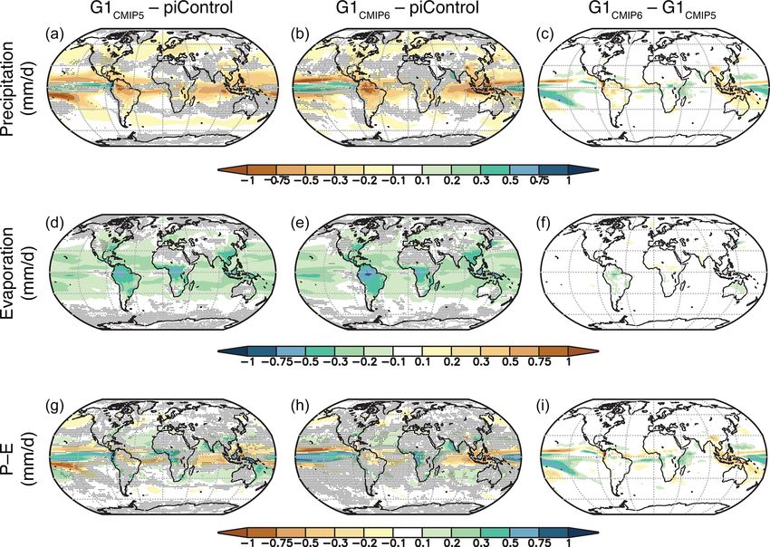
4232                                                                   B. Kravitz et al.: GeoMIP G1 in CMIP5 and CMIP6

the only tools for understanding the climatic consequences         models (Kravitz et al., 2015). As such, this is an opportu-
of solar geoengineering. In model simulations of solar geo-        nity to revisit some central questions in solar geoengineering.
engineering, insolation reduction is often used as a proxy         Many of the CMIP5 results regarding solar geoengineering
for actual stratospheric sulfate aerosols, as it captures many     showed substantial agreement across the participating Ge-
of the broad radiative effects of stratospheric aerosol geo-       oMIP models. In this newest iteration of GeoMIP, do the
engineering as well as some of the important climate effects       same science conclusions still hold, and do the models still
like surface cooling and hydrological cycle strength reduc-        generally agree on the resulting climate effects? Here, we
tion (Niemeier et al., 2013; Kalidindi et al., 2015). However,     address these questions by evaluating and comparing gen-
stratospheric sulfate aerosols also absorb longwave radiative      eral climate model response to GeoMIP experiment G1 (de-
flux, which heats the upper troposphere and lower strato-          scribed in the next section) from both CMIP5 and CMIP6.
sphere. As such, any implementation of stratospheric geo-
engineering with sulfate aerosols would produce additional
effects, such as changing atmospheric circulation in response      2   Simulations and participating models
to stratospheric heating and heating gradients (e.g., Richter
et al., 2017; Tilmes et al., 2018; Simpson et al., 2019) and       In this study, we evaluate GeoMIP experiment G1, in which,
stratospheric ozone changes (e.g., Pitari et al., 2014), as well   starting from a pre-industrial control (piControl) base-
as changes in ultraviolet radiative flux and enhanced diffuse      line, the atmospheric CO2 concentration is instantaneously
radiation at the surface (Madronich et al., 2018). However,        quadrupled (the standard CMIP experiment abrupt4xCO2),
here we consider the major, large-scale effect of reflecting       and insolation is simultaneously reduced such that net top-
sunlight to cool Earth.                                            of-atmosphere (TOA) radiative flux is within ±0.1 W m−2 of
   Simulations of solar geoengineering with solar reduction        the baseline value in the first decade of simulation (Kravitz
have long shown that solar geoengineering would cool the           et al., 2011, 2015). This experiment was part of the origi-
planet, offsetting global warming (e.g., Govindasamy and           nal suite of GeoMIP experiments and was repeated and ex-
Caldeira, 2000; NRC, 2015; Irvine et al., 2016), although          tended in the newest suite in an effort to understand the role
there would still be residual regional effects (e.g., Kravitz      of model structural uncertainty in broad conclusions about
et al., 2014). Idealized simulations of solar reduction have       solar geoengineering. Participating models are listed in Ta-
also been simulated in a multi-model context under the             ble 1. We include 13 models from CMIP5 and 7 models from
Geoengineering Model Intercomparison Project (GeoMIP;              CMIP6. Experiment G1 is an idealized experiment aimed at
Kravitz et al., 2011), to understand the robust model re-          understanding physical climate response and not as a pro-
sponses to various standardized solar geoengineering sim-          posed real-world geoengineering implementation. Although
ulation designs. Multi-model conclusions from these stud-          G1 should not be used directly for impacts analysis, im-
ies indicate that solar geoengineering would be effective          proved understanding of climate model response to G1 will
at partially offsetting greenhouse-gas-induced temperature         increase confidence when evaluating more policy-relevant
changes (Kravitz et al., 2013a), as well as changes in the hy-     scenarios.
drological cycle (Tilmes et al., 2013), the cryosphere (Moore         The original G1 experiment was 50 years in length,
et al., 2014), extreme events (Curry et al., 2014; Aswathy         whereas the CMIP6 version is 100 years in length to
et al., 2015), vegetation (Glienke et al., 2015), circulation      allow for better analyses of rare events and to capture
(Guo et al., 2018; Gertler et al., 2020), agricultural yield po-   very slow responses. Comparison between the two ensem-
tential (Xia et al., 2014), and numerous other areas. However,     bles necessitates only using the first 50 years, but we
the offset is not exact (Moreno-Cruz et al., 2012), particularly   need to verify that this can be done without losing im-
on a regional basis or when considering multiple simultane-        portant longer-term evolution in features. Figures 1 and 2
ous metrics of climate change (Kravitz et al., 2014; Irvine        look at G1 behavior over the entire 100-year period of
et al., 2019), leading to concerns about winners and losers        the CMIP6 simulations to determine whether there is any
from geoengineering (Ricke et al., 2010). To some extent, the      drift or steady-state error that would not be revealed by
effects of solar geoengineering may be tailored or designed        only analyzing the first 50 years. (Also see Table 2 for
(MacMartin et al., 2013; Kravitz et al., 2016, 2017, 2019),        quantitative information.) Over years 11–100 of simula-
but solar geoengineering will still not be able to completely      tion, CNRM-ESM2.1 and IPSL-CM6A-LR show negative
offset climate change from greenhouse gases.                       trends in temperature greater than 0.1 K decade−1 in magni-
   The previous phase of GeoMIP was associated with the            tude, and CESM2(WACCM) and UKESM1.0-LL shows pos-
CMIP5 (Taylor et al., 2012), an international collaboration        itive trends of similar magnitudes. This is despite no model
of climate models to attempt to understand robust model re-        showing a trend in net TOA radiative flux greater in mag-
sponses to various forcings. GeoMIP has now entered a new          nitude than 0.02 W m−2 decade−1 . Beyond an initial tran-
phase, concurrent with CMIP6 (CMIP6; Eyring et al., 2016),         sient period, CESM2(WACCM), CNRM-ESM2.1, and IPSL-
and with it are new solar geoengineering simulations with          CM6A-LR show approximately 0.06 % decade−1 trends in
new and updated versions of the participating Earth system         precipitation and evaporation of the same sign as the temper-

Atmos. Chem. Phys., 21, 4231–4247, 2021                                             https://doi.org/10.5194/acp-21-4231-2021
B. Kravitz et al.: GeoMIP G1 in CMIP5 and CMIP6                                                                                            4233

Table 1. All participating models in both the CMIP5 and CMIP6 eras of GeoMIP, including references. For G1 solar reduction, the percentage
is calculated as the percent change in incident solar irradiance at the TOA between G1 and its respective piControl run. Numbers in the first
column correspond to the model numbers in Fig. 11.

 No.    Model                  Generation    Reference                             G1 solar   Data not         Data citations
                                                                              reduction (%)   available        (CMIP6 only)
 1      BNU-ESM                CMIP5         Ji et al. (2014)                          3.80   Cloud forcing
 2      CanESM2                CMIP5         Arora et al. (2011)                       4.00
 3      CCSM4                  CMIP5         Gent et al. (2011)                        4.25   NPP
 4      CESM-CAM5.1-FV         CMIP5         Neale et al. (2010),                      4.70
                                             Hurrell et al. (2013)
 5      CSIRO-Mk3L-1.2         CMIP5         Phipps et al. (2011, 2012)                3.20   Cloud forcing,
                                                                                              NPP
 6      EC-EARTH               CMIP5         Hazeleger et al. (2011)                   4.12   Cloud forcing,
                                                                                              NPP
 7      GISS-E2-R              CMIP5         Schmidt et al. (2014)                     4.47
 8      HadCM3                 CMIP5         Gordon et al. (2000)                      4.16   Cloud forcing,
                                                                                              NPP
 9      HadGEM2-ES             CMIP5         Collins et al. (2011)                     3.88
 10     IPSL-CM5A-LR           CMIP5         Dufresne et al. (2013),                   3.50   NPP
                                             Hourdin et al. (2012)
 11     MIROC-ESM              CMIP5         Watanabe et al. (2008, 2011)              5.00
 12     MPI-ESM-LR             CMIP5         Giorgetta et al. (2013),                  4.68
                                             Stevens et al. (2013)
 13     NorESM1-M              CMIP5         Alterskjær et al. (2012),                 4.03
                                             Kirkevåg et al. (2013)
 14     CanESM5                CMIP6         Swart et al. (2019c)                      3.72                    Swart et al. (2019a, b),
                                                                                                               Cole et al. (2019)
 15     CESM2-WACCM            CMIP6         Gettelman et al. (2019)                   4.91                    Danabasoglu (2019a, b, c)
 16     CNRM-ESM2.1            CMIP6         Séférian et al. (2019)                    3.72                    Séférian (2018a, b, c)
 17     GISS-E2.1-G            CMIP6         Kelley et al. (2020)                      4.13                    NASA Goddard Institute for
                                                                                                               Space Studies (NASA/GISS)
                                                                                                               (2019, 2018)
 18     IPSL-CM6A-LR           CMIP6         Boucher et al. (2020),                    4.10                    Boucher et al. (2018a, b, c)
                                             Lurton et al. (2020)
 19     MPI-ESM1.2-LR          CMIP6         Mauritsen et al. (2019)                   4.57                    Wieners et al. (2019a, b)
 20     UKESM1.0-LL            CMIP6         Sellar et al. (2019)                      3.80                    Tang et al. (2019a, b),
                                                                                                               Jones (2019)

ature trends. Nevertheless, the differences in temperature and              has a steadily increasing temperature value, possibly related
hydrological cycle change due to experiment G1 are orders                   to a slight trend in sea ice coverage (Boucher et al., 2020).
of magnitude greater than the calculated values in Table 2.                    IPSL-CM6A-LR is also known to have a bicentennial os-
As such, we conclude that our choice to focus on the first                  cillation, which could affect G1–piControl differences, de-
50 years of simulation does not appreciably affect our results.             pending on the baseline period used for subtraction. To ver-
   Figure 2 shows that many of the models have low-                         ify that this oscillation is not impacting our results, we di-
frequency variability that appears in the different regions                 vided that model’s 1200-year piControl run into 50-year
plotted here. For the region north of 30◦ N, IPSL-CM6A-LR                   chunks and computed the surface air temperature average
                                                                            for each of those chunks. The largest temperature found was

https://doi.org/10.5194/acp-21-4231-2021                                                      Atmos. Chem. Phys., 21, 4231–4247, 2021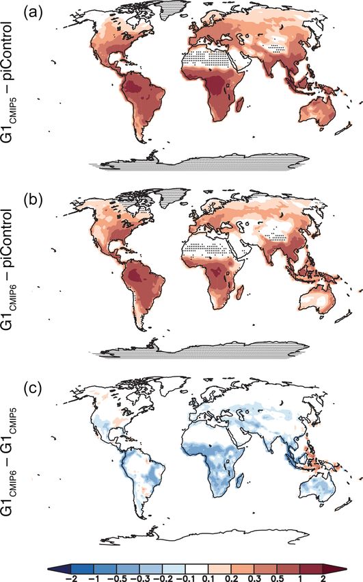
4234                                                                          B. Kravitz et al.: GeoMIP G1 in CMIP5 and CMIP6

Table 2. Decadal trends in the global mean temperature, net TOA radiative flux, precipitation, and evaporation values shown in Fig. 1 for
each model. Trends are calculated across the years 11–100 to eliminate any effects due to initial transient adjustment to the abrupt forcing.

                       Model                   Temperature             Rad. flux       Precipitation    Evaporation
                                              (K decade−1 )    (W m−2 decade−1 )      (% decade−1 )    (% decade−1 )
                       CanESM5                       0.010                 −0.005            0.011            0.011
                       CESM2(WACCM)                  0.023                 −0.009            0.067            0.067
                       CNRM-ESM2.1                  −0.033                  0.016           −0.058           −0.058
                       GISS-E2.1-G                  −0.005                  0.018           −0.006           −0.006
                       IPSL-CM6A-LR                 −0.027                  0.015           −0.062           −0.063
                       MPI-ESM1.2-LR                −0.003                 −0.000           −0.015           −0.016
                       UKESM1.0-LL                   0.018                  0.008            0.018            0.018
                       Ensemble mean                −0.002                  0.006           −0.006           −0.007

Figure 1. Temperature (a; K), net top-of-atmosphere radiative flux (b; W m−2 ), precipitation (c; %), and evaporation (d; %) change in
G1CMIP6 compared to piControl over 100 years of simulation. Thin colored lines are individual models, and thick black lines are ensemble
means.

286.0339 K, and the smallest was 285.6384 K. The average                 the best match to the period covered by G1) yields a tem-
over the entire ensemble was 285.8604 K. As such, using the              perature of 285.9084 K, which is 0.048 K different from the
mean of the entire ensemble versus matching the appropriate              mean of the entire piControl run. As such, we conclude that
period in the bicentennial oscillation would have an impact              this bicentennial oscillation is unlikely to have substantially
on G1–piControl temperature by at most 0.22 K. Only aver-                influenced our findings.
aging the first 100 years of the piControl run (which may be

Atmos. Chem. Phys., 21, 4231–4247, 2021                                                     https://doi.org/10.5194/acp-21-4231-2021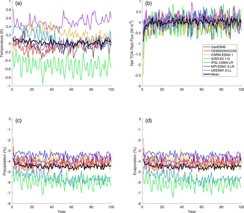
B. Kravitz et al.: GeoMIP G1 in CMIP5 and CMIP6                                                                                  4235

Figure 2. Annual mean surface temperature (K) in each model averaged over 90–30◦ S (a), 30◦ S–30◦ N (b), and 30–90◦ N (c). The ensemble
mean is plotted as thick black lines.

   Per the results in Fig. 1, IPSL-CM6A-LR and GISS-E2.1-                  cores, convective parameterizations, radiative transfer
G appear to have a different responsiveness of the hydrolog-               modules, terrestrial biosphere and cryosphere; Knutti
ical cycle to the combined CO2 –solar forcing than the other               et al., 2013; Zelinka et al., 2020), there have been nu-
models. We are reluctant to attribute this feature to any po-              merous developments in models in these areas (and oth-
tential shortcomings or lack of fidelity to observations be-               ers) between CMIP5 and CMIP6 such that in most cases
cause there are no observations of this type of experiment.                a direct comparison would not be meaningful.
Although these models are outliers, there is no evidential ba-
sis on which to assume they are more or less valid than the             – We focus extensively on the G1 results and, with
other models for this study.                                              few exceptions, do not focus on the corresponding
   Because the main focus of this paper is a comparison be-               abrupt4xCO2 simulations. It has been well documented
tween the CMIP5 and CMIP6 generations of model results,                   that the CMIP6 models tend to have higher climate sen-
we have opted for the following to aid comparisons:                       sitivities than the CMIP5 models (Flynn and Mauritsen,
                                                                          2020; Meehl et al., 2020; Zelinka et al., 2020), so we do
  – Since we are not evaluating any features that require
                                                                          not wish to make conclusions that might be based on a
    100 years of statistics, and the results do not show any
                                                                          form of selection bias.
    appreciable time evolution of behavior after the first
    couple of years (see discussion above), we only eval-
                                                                        – All lack of stippling on map plots, as in previous Ge-
    uate the first 50 years of all simulations. All maps show
                                                                          oMIP studies (e.g., Kravitz et al., 2013a), indicates
    changes over years 11–50, removing the initial transient
                                                                          agreement on the sign of the response in at least 75 %
    period.
                                                                          of models. Because G1CMIP5 has more participating
  – We do not compare previous versions of individual                     models than G1CMIP6 , this threshold provides some
    models with current ones, instead only examining en-                  consistency across analyses of the ensembles. When
    sembles. Even though models may share similar devel-                  plotting differences between the ensembles (G1CMIP6 –
    opment histories (e.g., atmosphere and ocean dynamical                G1CMIP5 ), there is no stippling, as it is difficult to mean-

https://doi.org/10.5194/acp-21-4231-2021                                               Atmos. Chem. Phys., 21, 4231–4247, 2021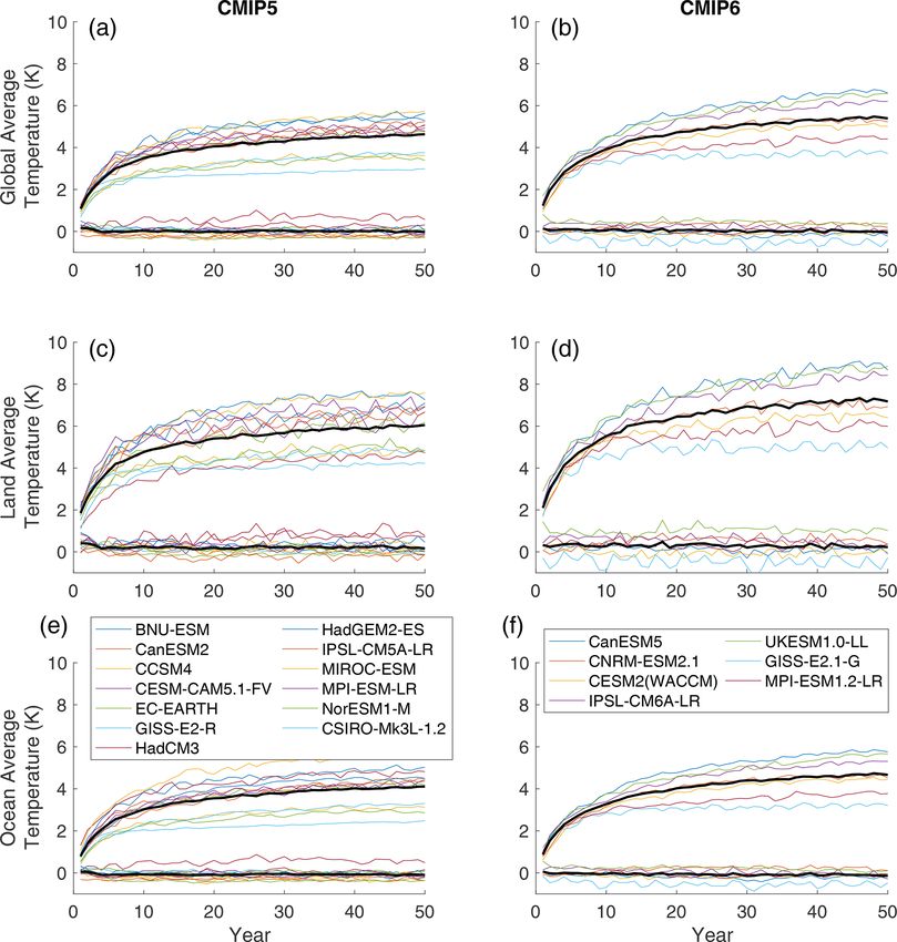
4236 B. Kravitz et al.: GeoMIP G1 in CMIP5 and CMIP6
ingfully represent such differences between ranges. Ag-
gregate differences between the two ensembles, as cal-
culated using Welch’s t test or differences in stippled
area, are discussed in Table 3.
For CMIP6, we analyzed one ensemble member for all
experiments except for CanESM5 (G1), CNRM-ESM2.1
(abrupt4xCO2 and G1), and UKESM1.0-LL (G1).
3 Results
3.1 Energetics
Ensemble mean radiative and turbulent flux quantities are
plotted in Fig. 3, and the ensemble ranges are plotted in
Fig. 4. An immediate observation is that, in both ensembles,
the models were successful at limiting net TOA radiative flux
change to within approximately ±0.1 W m−2 of the models’
respective pre-industrial values. Accomplishing this required
an average solar reduction of 4.14 % (models range within
3.20 %–5.00 %) in CMIP5 and 4.14 % (3.72 %–4.91 %) in
CMIP6. As such, despite numerous structural changes be-
tween the two generations of models, there is no appreciable
change in solar efficacy (Hansen et al., 2005).
None of the radiative flux quantities indicate large tran-
sients over 50 years of simulation of G1, other than the ini-
tial flux change within the first year or so of simulation.
This is consistent with the “perpetual fast response” found by
Kravitz et al. (2013b), in which because global mean temper-
ature does not change appreciably over the course of the G1 Figure 3. Ensemble mean energetics (W m−2 ) for various flux
simulation, climate feedbacks are not excited, and the inter- quantities in G1CMIP5 (a), G1CMIP6 (b), and their difference (c).
nal state of the system (as measured by, for example, fluxes All fluxes are positive downward, which is counterintuitive for sen-
and hydrological cycle changes) similarly does not change. sible heat (SH) and latent heat (LH). Surf energy budget indicates
Ensemble mean fluxes show few differences (< 1 W m−2 in the sum of surface shortwave (SW), surface longwave (LW), SH,
magnitude) with the exception of shortwave cloud forcing, and LH. Cloud forcing is calculated as all-sky minus clear-sky ra-
defined as all-sky minus clear-sky shortwave flux at the sur- diative flux.
face. On average, the CMIP6 ensemble has 3–4 W m−2 less
shortwave cloud forcing than CMIP5. Neglecting some out-
widespread result, but the most prominent features are in the
liers, for each flux except shortwave (and hence total) cloud
tropics, especially over the Amazon, Africa, and the Mar-
forcing, the median model in one ensemble is within the in-
itime Continent. These regions encompass tropical forests,
terquartile range of the other ensemble. This indicates that
indicating a potential for vegetation feedbacks on the tem-
there are no major differences between the ensembles in how
perature reductions. However, the reasons behind these forc-
the models handle energy balance and energetics, with the
ing changes are difficult to diagnose, as they could be due
exception of clouds, which is consistent with findings about
to changes in cloud thickness, cloud cover, or cloud level be-
CMIP6 (Zelinka et al., 2020). Moreover, it appears that most
tween CMIP5 and CMIP6 models (e.g., Vignesh et al., 2020),
of the major differences in shortwave cloud forcing are due
differences in how solar geoengineering affects clouds (Rus-
to outliers in each ensemble, which are positive for CMIP5
sotto and Ackerman, 2018), or artifacts of the analyses (e.g.,
and negative for CMIP6. To further explore these potential
cloud masking; Andrews et al., 2009; Kravitz et al., 2013b).
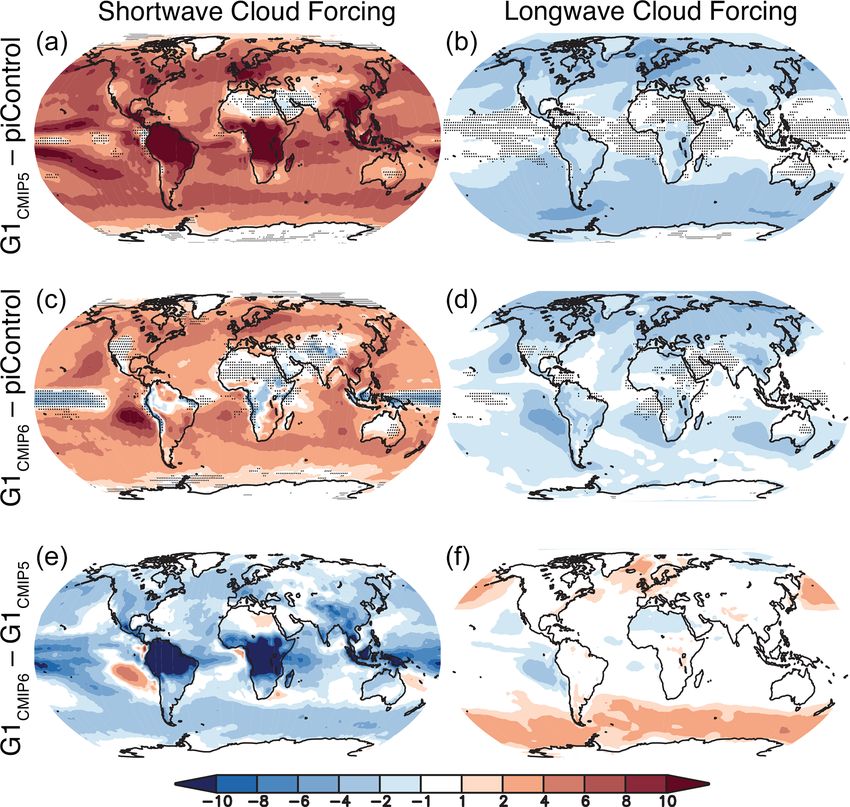
differences, Fig. 5 provides maps of the ensemble means for
Moreover, based on the results in Fig. 4, it is likely that many
cloud forcing. In G1, the CMIP5 ensemble showed more pos-
of these features are exaggerated by outlier models (also see
itive shortwave cloud forcing and more negative longwave
Vignesh et al., 2020). As such, we reserve such detailed in-
cloud forcing (i.e., more cancellation) than the CMIP6 en-
vestigations for future work.
semble. Overall, the CMIP6 ensemble has greatly reduced
(in some places by over 10 W m−2 ) shortwave cloud forcing
as compared to CMIP5 under the G1 experiment. This is a
Atmos. Chem. Phys., 21, 4231–4247, 2021 https://doi.org/10.5194/acp-21-4231-2021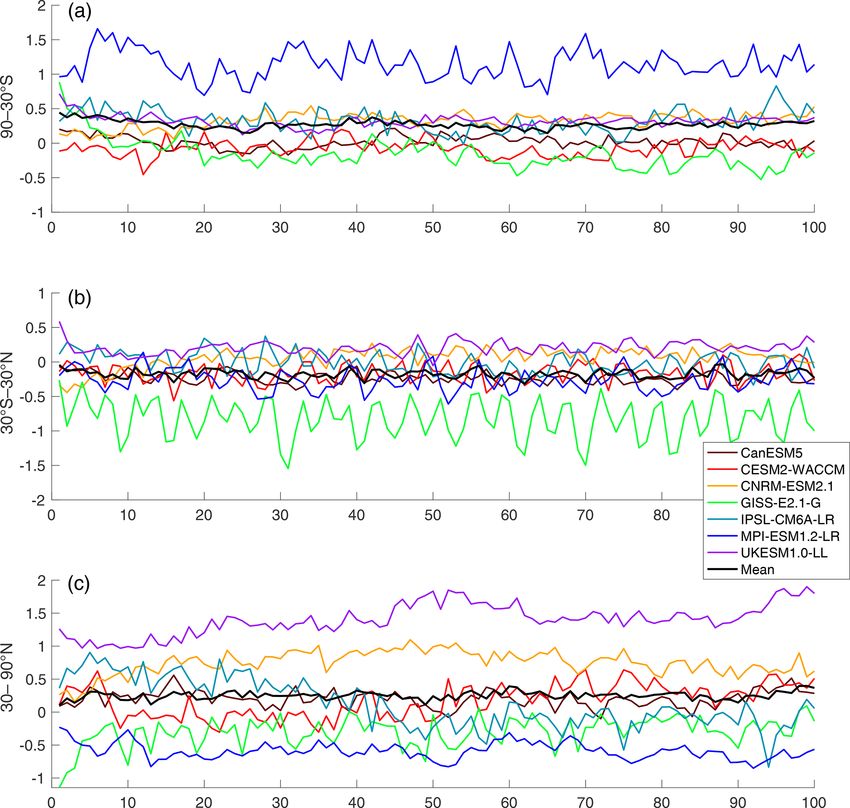
B. Kravitz et al.: GeoMIP G1 in CMIP5 and CMIP6                                                                                           4237

Table 3. Ensemble differences between the CMIP5 and CMIP6 ensembles for each variable evaluated in this study (left column). Column 2
indicates the difference between the ensembles in how much of the Earth’s surface is not stippled (more than 75 % of models agree on the
sign of the response; negative values indicate that CMIP6 has less unstippled area than CMIP5). Column 3 indicates the percent of the Earth’s
surface for which the CMIP5 ensemble is statistically different from the CMIP6 ensemble, based on 95th percentile confidence intervals from
Welch’s t test.

                           Variable                     Stippling (%)    Welch’s t test (%)     Notes
                           Surface air temperature            −25.77                   0.87
                           Precipitation                       −3.56                  11.17
                           Evaporation                         −2.33                   6.47
                           P –E                               −15.23                   1.13
                           SW cloud forcing                    −8.02                   9.65
                           LW cloud forcing                    11.99                   6.57
                           Net primary productivity            −1.42                   1.15     Land surface only

Figure 4. Ensemble median (red lines), interquartile (blue boxes),
and ranges (black whiskers) for the same global mean energetic
quantities as in Fig. 3 (G1 minus piControl) for both the CMIP5
and CMIP6 ensembles.
                                                                         Figure 5. Surface shortwave (a, c, e) and longwave (b, d, f)
                                                                         cloud forcing (W m−2 ) change from pre-industrial values for the
3.2   Temperature                                                        CMIP5 (a, b) and CMIP6 (c, d) ensembles, as well as the ensemble
                                                                         differences (e, f). Cloud forcing is measured as all-sky minus clear-
These small flux changes also led to few G1 temperature                  sky radiative flux. All shaded values are ensemble means. Lack of
changes between the two ensembles. Figure 6 shows global-,               stippling indicates agreement on the sign of the values across at least
land-, and ocean-averaged temperatures for the CMIP5 and                 75 % of the models.
CMIP6 ensembles. In general, the abrupt4xCO2 simulation
in CMIP6 has higher temperatures than in CMIP5, con-
sistent with the noted increase in climate sensitivity (Vial
et al., 2013; Flynn and Mauritsen, 2020; Meehl et al., 2020;                       Zπ/2
Zelinka et al., 2020). In both ensembles, G1 is effective at                  1
                                                                         T0 =             T (ψ) dA
offsetting global mean temperature change, in some cases                      A
with a slight positive residual temperature change over land.                     −π/2
Figure 7 shows three aggregate temperature metrics: global                         Zπ/2
mean temperature (T0 ), the interhemispheric temperature                      1
                                                                         T1 =             T (ψ) sin ψ dA
gradient (T1 ), and the Equator-to-pole temperature gradient                  A
                                                                                  −π/2
(T2 ) (Ban-Weiss and Caldeira, 2010; Kravitz et al., 2016):
                                                                                   Zπ/2
                                                                              1                1
                                                                         T2 =             T (ψ) (3sin2 ψ − 1) dA,                           (1)
                                                                              A                2
                                                                                  −π/2

https://doi.org/10.5194/acp-21-4231-2021                                                      Atmos. Chem. Phys., 21, 4231–4247, 2021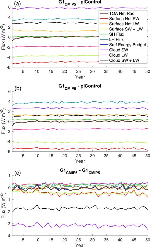
4238 B. Kravitz et al.: GeoMIP G1 in CMIP5 and CMIP6
Figure 6. Global mean (a, b), land mean (c, d), and ocean mean (e, f) temperature change (K) for the CMIP5 (a, c, e) and CMIP6 (b, d, f).
Thin colored lines are individual models, and thick black lines are model means. In all panels, the upper cluster of lines is the abrupt4xCO2
simulation, and the lower cluster of lines (approximately zero temperature change for the entire simulation) is experiment G1.
where A is area. As for the fluxes, the median model in one the poles (Govindasamy and Caldeira, 2000; Kravitz et al.,
ensemble is within the interquartile range of the other ensem- 2013a). CMIP6 shows slightly less high-latitude warming
ble. This indicates that no ensemble is on average warmer than CMIP5, but temperature differences between the two
or cooler than another, has a substantially warmer Northern ensembles are largely negligible. However, the warmer tem-
or Southern Hemisphere than the other, nor warmer tropics peratures in CMIP6 near Greenland have important impli-
or poles than the other. We can conclude that spatial pat- cations for ice sheet melt and consequent sea level rise, as
terns of temperature change from G1 are robust across a wide well as bottom water formation. We reserve such analyses
range of structural uncertainty, including an increase in cli- for future investigations, particularly since the models used
mate sensitivity between the two generations of CMIP. here are not capable of simulating the eustatic component of
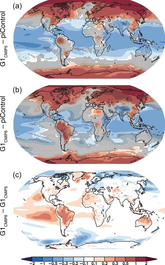
The spatial structure of temperature change (Fig. 8) does sea level rise. In any case, these ensemble mean differences
have small differences between the two ensembles. G1 in between CMIP5 and CMIP6 cannot be deemed statistically
CMIP6 has multiple locations that are warmer than G1 in significant (Table 3 and Fig. 7).
CMIP5, despite both ensembles achieving net energy bal-
ance at TOA and the surface (Fig. 3). The majority of 3.3 Hydrological and other integrative changes
the differences are over land and in the tropics, where
CMIP6 is slightly warmer than CMIP5 (up to 1 ◦ C in some
Figure 9 shows ensemble mean changes in precipitation (P ),
places). Nevertheless, both ensembles show the well-noted
evaporation (E), and P –E for G1CMIP5 and G1CMIP6 . Qual-
feature that offsetting a CO2 increase with globally uni-
itatively, patterns are similar between both ensembles. Pre-
form solar reduction overcools the tropics and undercools
cipitation is slightly (< 0.3 mm d−1 in magnitude) differ-
Atmos. Chem. Phys., 21, 4231–4247, 2021 https://doi.org/10.5194/acp-21-4231-2021B. Kravitz et al.: GeoMIP G1 in CMIP5 and CMIP6 4239
Figure 7. Ensemble ranges for global mean temperature (T0 ), the
interhemispheric temperature gradient (T1 ), and the Equator-to-pole
temperature gradient (T2 ), as defined in Eq. (1) (Ban-Weiss and
Caldeira, 2010; Kravitz et al., 2016). Red lines indicate ensemble
medians, blue boxes are the interquartile ranges, and black whiskers Figure 8. Ensemble average temperature changes (K) for G1
indicate total ranges. (as compared to the pre-industrial control) for CMIP5 (a)
and CMIP6 (b), as well as their difference (G1CMIP6 minus
G1CMIP5 , c). In panels (a) and (b), stippling indicates regions where
fewer than 75 % of the models in their respective ensembles agree
on the sign of the response.
ent in the tropics between the two ensembles. The major-
ity of those features can be summarized as a more south-
ward Intertropical Convergence Zone (ITCZ), more precipi- in both global mean temperature and global mean precipita-
tation in the South Pacific Convergence Zone, and less pre- tion.
cipitation over southeast Asia and the Maritime Continent in As an integrator of CO2 , temperature, and precipitation ef-
G1CMIP6 . Evaporation in the two ensembles is nearly identi- fects over land, Fig. 12 shows changes in terrestrial net pri-
cal except for more evaporation in Amazonia and Australia mary productivity (NPP). Numerous land regions have lower
in G1CMIP6 . As such, the net P –E change between the two NPP in CMIP6 than in CMIP5. The ensemble average global
ensembles strongly resembles the precipitation changes. Fig- NPP change (G1–piControl) is 51.2 (4.1–122.1) Pg C yr−1 in
ure 10 shows that, like previous evaluations of ensemble CMIP5 and 38.1 (19.5–77.5) Pg C yr−1 in CMIP6, represent-
ranges, the median model in one ensemble falls well within ing a 25.6 % difference in means. Jones et al. (2013) used
the interquartile range of the other ensemble for P , E, and NPP to highlight the importance of understanding the influ-
P –E. As such, we cannot conclude any robust hydrological ence of structural land model differences on climate results
cycle changes between the two ensembles. related to geoengineering. While it is beyond the scope of
Figure 11 shows average (years 11–50) temperature this study to perform a detailed diagnosis of which uncer-
change (with respect to piControl) plotted against average tainties or processes are responsible for this inter-ensemble
precipitation change for each model, as in Tilmes et al. difference (and indeed the present setup does not allow for
(2013). Other than a potentially greater climate sensitivity of a controlled experiment to rigorously test structural uncer-
some CMIP6 models, there is no distinguishable difference tainty), we show that the ensemble spread of total terres-
in aggregate behavior between the two ensembles. The same trial NPP is smaller in CMIP6 than in CMIP5. This result is
conclusion discovered by Tilmes et al. (2013) holds: solar re- consistent with the recent assessment of carbon cycle feed-
duction cannot simultaneously offset CO2 -induced changes backs conducted by Arora et al. (2020), who showed that the
https://doi.org/10.5194/acp-21-4231-2021 Atmos. Chem. Phys., 21, 4231–4247, 20214240 B. Kravitz et al.: GeoMIP G1 in CMIP5 and CMIP6
Figure 9. Precipitation (a–c), evaporation (d–f), and precipitation minus evaporation (P –E; g–i) change from pre-industrial values for the
CMIP5 (a, d, g) and CMIP6 (b, e, h) ensembles, as well as the ensemble differences (c, f, i). All shaded values are ensemble means. Lack of
stippling in the left and middle panels indicates agreement on the sign of the values across at least 75 % of the models.
CMIP6 ensemble has reduced overall model spread in the
land carbon cycle to rising CO2 compared to their CMIP5
predecessors.
4 Discussion and conclusions
Based on the results presented here, model response to G1
has not changed substantially between CMIP5 and CMIP6,
despite numerous changes to models between the two gener-
ations, including an increase in climate sensitivity. The signs
of residual climate impacts (for example, in temperature) are
in better agreement in CMIP5 than CMIP6 (Table 3 shows
a difference in stippled area between the two ensembles),
but this could be a function of the smaller ensemble size
in CMIP6. Alternatively, the factors affecting the signs of
Figure 10. Global mean ensemble median (red lines), interquar- residual climate impacts are not understood well enough for
tile (blue boxes), and ranges (black whiskers or, for P –E, one blue the CMIP6 models to show improvement over CMIP5. En-
circle indicating an extreme outlier) for the hydrological quantities ergetics, temperature, and the hydrological cycle are qualita-
shown in Fig. 9 for both the CMIP5 and CMIP6 ensembles. tively and quantitatively similar in both ensemble means and
ensemble ranges, although these variables are somewhat re-
lated, so we might expect them to all portray a similar picture.
Notable differences do exist in shortwave cloud forcing and
Atmos. Chem. Phys., 21, 4231–4247, 2021 https://doi.org/10.5194/acp-21-4231-2021B. Kravitz et al.: GeoMIP G1 in CMIP5 and CMIP6 4241
Figure 11. Average (years 11–50) temperature (y axis; K) and pre-
cipitation (x axis; %) change for each model in this study. Numbers
indicate the model number (listed in Table 1, first column). Black
numbers are for abrupt4xCO2, and red numbers are for G1. Bolded
numbers are for CMIP6.
NPP, particularly in Amazonia, Africa, and Australia, which
are also regions of inter-ensemble difference in precipitation.
From these findings, we can conclude that results obtained
Figure 12. Terrestrial net primary productivity (kg C m−2 yr−1 ) for
over two generations of models have not been overturned by
the CMIP5 (a) and CMIP6 (b) ensembles, as well as the ensemble
the latest round of simulations. All of the major ensemble dif- differences (c). All shaded values are ensemble means. Lack of stip-
ferences highlighted above deal with clouds and land surface pling indicates agreement on the sign of the values across at least
modeling, both of which are difficult to model and are neces- 75 % of the models.
sarily highly parameterized. The conclusions that are based
on more fundamental knowledge, such as column energetics
(in the case of the hydrological cycle), are relatively robust sequences of stratospheric heating like the positive winter-
to structural uncertainty, insofar as this study adequately cap- time North Atlantic Oscillation; Simpson et al., 2019; Jones
tures representative variations in structural uncertainty. This et al., 2021) require detailed assessments with state-of-the-
lends confidence to our conclusions about the broad climate art aerosol microphysical schemes. This is particularly im-
effects from modeling solar geoengineering via solar dim- portant for understanding regional and seasonal solar geo-
ming. engineering (Kravitz et al., 2017; Visioni et al., 2019). Such
We also conclude that the models used in CMIP5 are not detailed microphysical calculations can only be simulated in
obviously biased or inferior as compared to CMIP6. While a small number of models; in the case of Jones et al. (2021),
improvements have been made in the CMIP6 generation of only two models were available. While simple G1-style ex-
models, and those models are likely better for representing periments enable a robust multi-model ensemble analysis,
numerous features of the present-day climate that may be they cannot capture details that depend on microphysics.
important for studies of geoengineering, there are many as- We emphasize the importance of a variety of modeling ap-
pects of climate that are well represented by earlier mod- proaches to understand solar geoengineering, particularly the
els. In some cases, more robust analyses may be enabled by role of model uncertainty in conclusions about solar geoengi-
augmenting ensemble sizes with archived output from earlier neering.
generations of CMIP models. There are numerous aspects of physical climate that we
Many of the broad features of solar geoengineering with did not evaluate, nor did we pursue analyses beyond physical
sulfate aerosols can be represented by a reduction in solar climate, including many other aspects of natural science, so-
constant (e.g., Niemeier et al., 2013; Kalidindi et al., 2015). cial science, the humanities, governance, justice, or ethics (to
However, the more subtle changes that derive from complex name a few important areas). Moreover, we emphasize that
response to stratospheric aerosol heating (for example, con- experiment G1 is an idealized experiment aimed at under-
https://doi.org/10.5194/acp-21-4231-2021 Atmos. Chem. Phys., 21, 4231–4247, 20214242 B. Kravitz et al.: GeoMIP G1 in CMIP5 and CMIP6
standing physical climate response to combinations of large is supported by NSF grant nos. AGS-1617844 and AGS-2017113.
forcings and should not be interpreted as a realistic or policy- Jim Haywood and Andy Jones were supported by the Met Of-
relevant scenario of geoengineering. A holistic assessment fice Hadley Centre Climate Programme funded by BEIS and De-
of the consequences of geoengineering, particularly of more fra. Ulrike Niemeier is supported by the German DFG-funded
policy-relevant scenarios, would certainly need to take these Research Unit VollImpact FOR2820 subproject no. TI344/2-1
and MPIESM simulation have been performed on the computer
numerous aspects into account. Nevertheless, based on the
of Deutsches Klimarechenzentrum (DKRZ). Olivier Boucher and
results presented here, results for geoengineering across sev- Thibaut Lurton were supported by the IPSL Climate Gradu-
eral important metrics appear to be consistent across some ate School EUR (ANR grant no. ANR-11-IDEX-0004-17-EURE-
important structural uncertainties. This lends confidence to 0006). The CMIP6 project at IPSL used the HPC resources of
some conclusions drawn from global climate models regard- TGCC under allocations 2016-A0030107732, 2017-R0040110492,
ing solar geoengineering. and 2018-R0040110492 (project gencmip6) provided by GENCI
(Grand Équipement National de Calcul Intensif). Roland Séférian
and Pierre Nabat were supported by the H2020 CONSTRAIN un-
Data availability. All CMIP5 and CMIP6 output, including the der the grant agreement no. 820829 and the Météo-France/DSI su-
respective GeoMIP simulations, is available via the Earth Sys- percomputing center.
tem Grid Federation (https://esgf-node.llnl.gov/projects/esgf-llnl/,
Lawrence Livermore National Laboratory, 2021) or by contact-
ing the respective modeling groups responsible for the output. For Review statement. This paper was edited by Xiaohong Liu and re-
CMIP6 output, see data citations in Table 1. viewed by Ralph Kahn and three anonymous referees.
Author contributions. BK, OB, JNSC, JH, AJ, TL, PN, UN, RS,
and ST contributed model output. BK performed the analysis. BK, References
DGM, and DV wrote the manuscript with all co-authors.
Alterskjær, K., Kristjánsson, J. E., and Seland, Ø.: Sensitivity
to deliberate sea salt seeding of marine clouds – observations
and model simulations, Atmos. Chem. Phys., 12, 2795–2807,
Competing interests. The authors declare that they have no conflict
https://doi.org/10.5194/acp-12-2795-2012, 2012.
of interest.
Andrews, T., Forster, P. M., and Gregory, J. M.: A surface en-
ergy perspective on climate change, J. Climate, 22, 2557–2570,
https://doi.org/10.1175/2008JCLI2759.1, 2009.
Special issue statement. This article is part of the special issue “Re- Arora, V. K., Scinocca, J. F., Boer, G. J., Christian, J. R., Denman,
solving uncertainties in solar geoengineering through multi-model K. L., Flato, G. M., Kharin, V. V., Lee, W. G., and Merryfield,
and large-ensemble simulations (ACP/ESD inter-journal SI)”. It is W. J.: Carbon emission limits required to satisfy future repre-
not associated with a conference. sentative concentration pathways of greenhouse gases, Geophys.
Res. Lett., 38, L05805, https://doi.org/10.1029/2010GL046270,
2011.
Acknowledgements. We acknowledge the World Climate Research Arora, V. K., Katavouta, A., Williams, R. G., Jones, C. D., Brovkin,
Programme, which, through its Working Group on Coupled Mod- V., Friedlingstein, P., Schwinger, J., Bopp, L., Boucher, O., Cad-
elling, coordinated and promoted CMIP. We thank the climate mod- ule, P., Chamberlain, M. A., Christian, J. R., Delire, C., Fisher,
eling groups for producing and making available their model output, R. A., Hajima, T., Ilyina, T., Joetzjer, E., Kawamiya, M., Koven,
the Earth System Grid Federation (ESGF) for archiving the data and C. D., Krasting, J. P., Law, R. M., Lawrence, D. M., Lenton,
providing access, and the multiple funding agencies who support A., Lindsay, K., Pongratz, J., Raddatz, T., Séférian, R., Tachiiri,
CMIP6 and ESGF. We also thank all participants of the Geoengi- K., Tjiputra, J. F., Wiltshire, A., Wu, T., and Ziehn, T.: Carbon–
neering Model Intercomparison Project and their model develop- concentration and carbon–climate feedbacks in CMIP6 models
ment teams. and their comparison to CMIP5 models, Biogeosciences, 17,
4173–4222, https://doi.org/10.5194/bg-17-4173-2020, 2020.
Aswathy, V. N., Boucher, O., Quaas, M., Niemeier, U., Muri, H.,
Financial support. Support for Ben Kravitz was provided in part Mülmenstädt, J., and Quaas, J.: Climate extremes in multi-model
by the National Science Foundation (NSF) through agreement simulations of stratospheric aerosol and marine cloud brighten-
no. CBET-1931641, the Indiana University Environmental Re- ing climate engineering, Atmos. Chem. Phys., 15, 9593–9610,
silience Institute, and the Prepared for Environmental Change https://doi.org/10.5194/acp-15-9593-2015, 2015.
Grand Challenge initiative. The Pacific Northwest National Lab- Ban-Weiss, G. A. and Caldeira, K.: Geoengineering as an
oratory is operated for the US Department of Energy by Battelle optimization problem, Environ. Res. Lett., 5, 031001,
Memorial Institute under contract no. DE-AC05-76RL01830. Re- https://doi.org/10.1088/1748-9326/5/3/034009, 2010.
sources supporting this work were provided by the NASA High-End Boucher, O., Denvil, S., Caubel, A., and Foujols, M. A.:
Computing (HEC) Program through the NASA Center for Climate IPSL IPSL-CM6A-LR model output prepared for
Simulation (NCCS) at Goddard Space Flight Center. Alan Robock CMIP6 GeoMIP G1, Earth System Grid Federation,
https://doi.org/10.22033/ESGF/CMIP6.5054, 2018a.
Atmos. Chem. Phys., 21, 4231–4247, 2021 https://doi.org/10.5194/acp-21-4231-2021B. Kravitz et al.: GeoMIP G1 in CMIP5 and CMIP6 4243
Boucher, O., Denvil, S., Caubel, A., and Foujols, M. A.: Danabasoglu, G.: NCAR CESM2-WACCM model output prepared
IPSL IPSL-CM6A-LR model output prepared for CMIP6 for CMIP6 CMIP abrupt-4xCO2, Earth System Grid Federation,
CMIP abrupt-4xCO2, Earth System Grid Federation, https://doi.org/10.22033/ESGF/CMIP6.10039, 2019b.
https://doi.org/10.22033/ESGF/CMIP6.5109, 2018b. Danabasoglu, G.: NCAR CESM2-WACCM-FV2 model output pre-
Boucher, O., Denvil, S., Caubel, A., and Foujols, M. A.: pared for CMIP6 CMIP piControl, Earth System Grid Federa-
IPSL IPSL-CM6A-LR model output prepared for tion, https://doi.org/10.22033/ESGF/CMIP6.11302, 2019c.
CMIP6 CMIP piControl, Earth System Grid Federation, Dufresne, J.-L., Foujols, M.-A., Denvil, S., Caubel, A., Marti, O.,
https://doi.org/10.22033/ESGF/CMIP6.5251, 2018c. Aumont, O., Balkanski, Y., Bekki, S., Bellenger, H., Benshila,
Boucher, O., Servonnat, J., Albright, A. L., Aumont, O., Balkan- R., Bony, S., Bopp, L., Braconnot, P., Brockmann, P., Cadule,
ski, Y., Bastrikov, V., Bekki, S., Bonnet, R., Bony, S., Bopp, L., P., Cheruy, F., Codron, F., Cozic, A., Cugnet, D., de Noblet,
Braconnot, P., Brockmann, P., Cadule, P., Caubel, A., Cheruy, N., Duvel, J.-P., Ethé, C., Fairhead, L., Fichefet, T., Flavoni,
F., Codron, F., Cozic, A., Cugnet, D., D’Andrea, F., Davini, S., Friedlingstein, P., Grandpeix, J.-Y., Guez, L., Guilyardi, E.,
P., de Lavergne, C., Denvil, S., Deshayes, J., Devilliers, M., Hauglustaine, D., Hourdin, F., Idelkadi, A., Ghattas, J., Jous-
Ducharne, A., Dufresne, J.-L., Dupont, E., Éthé, C., Fairhead, L., saume, S., Kageyama, M., Krinner, G., Labetoulle, S., Lahel-
Falletti, L., Flavoni, S., Foujols, M.-A., Gardoll, S., Gastineau, lec, A., Lefebvre, M.-P., Lefevre, F., Levy, C., Li, Z. X., Lloyd,
G., Ghattas, J., Grandpeix, J.-Y., Guenet, B., Guez, L., Guilyardi, J., Lott, F., Madec, G., Mancip, M., Marchand, M., Masson, S.,
E., Guimberteau, M., Hauglustaine, D., Hourdin, F., Idelkadi, A., Meurdesoif, Y., Mignot, J., Musat, I., Parouty, S., Polcher, J., Rio,
Joussaume, S., Kageyama, M., Khodri, M., Krinner, G., Lebas, C., Schulz, M., Swingedouw, D., Szopa, S., Talandier, C., Terray,
N., Levavasseur, G., Lévy, C., Li, L., Lott, F., Lurton, T., Luys- P., Viovy, N., and Vuichard, N.: Climate change projections using
saert, S., Madec, G., Madeleine, J.-B., Maignan, F., Marchand, the IPSL-CM5 Earth System Model: From CMIP3 to CMIP5,
M., Marti, O., Mellul, L., Meurdesoif, Y., Mignot, J., Musat, I., Clim. Dynam., 40, 2123–2165, https://doi.org/10.1007/s00382-
Ottlé, C., Peylin, P., Planton, Y., Polcher, J., Rio, C., Rochetin, N., 012-1636-1, 2013.
Rousset, C., Sepulchre, P., Sima, A., Swingedouw, D., Thiéble- Eyring, V., Bony, S., Meehl, G. A., Senior, C. A., Stevens, B.,
mont, R., Traore, A. K., Vancoppenolle, M., Vial, J., Vialard, Stouffer, R. J., and Taylor, K. E.: Overview of the Coupled
J., Viovy, N., and Vuichard, N.: Presentation and evaluation of Model Intercomparison Project Phase 6 (CMIP6) experimen-
the IPSL-CM6A-LR climate model, J. Adv. Model. Earth Sy., tal design and organization, Geosci. Model Dev., 9, 1937–1958,
12, e2019MS002010, https://doi.org/10.1029/2019MS002010, https://doi.org/10.5194/gmd-9-1937-2016, 2016.
2020. Flynn, C. M. and Mauritsen, T.: On the climate sensitiv-
Budyko, M. I.: Climatic Changes, American Geophysical Union, ity and historical warming evolution in recent coupled
Washington, DC, 1977. model ensembles, Atmos. Chem. Phys., 20, 7829–7842,
Cole, J. N., Swart, N. C., Kharin, V. V., Lazare, M., Scinocca, https://doi.org/10.5194/acp-20-7829-2020, 2020.
J. F., Gillett, N. P., Anstey, J., Arora, V., Christian, J. R., Jiao, Gent, P. R., Danabasoglu, G., Donner, L. J., Holland, M. M., Hunke,
Y., Lee, W. G., Majaess, F., Saenko, O. A., Seiler, C., Seinen, E. C., Jayne, S. R., Lawrence, D. M., Neale, R. B., Rasch, P. J.,
C., Shao, A., Solheim, L., von Salzen, K., Yang, D., Winter, Vertenstein, M., Worley, P. H., Yang, Z.-L., and Zhang, M.: The
B., and Sigmond, M.: CCCma CanESM5 model output pre- Community Climate System Model Version 4, J. Climate, 24,
pared for CMIP6 GeoMIP G1, Earth System Grid Federation, 4973–4991, https://doi.org/10.1175/2011JCLI4083.1, 2011.
https://doi.org/10.22033/ESGF/CMIP6.3158, 2019. Gertler, C. G., O’Gorman, P. A., Kravitz, B., Moore, J. C., Phipps,
Collins, W. J., Bellouin, N., Doutriaux-Boucher, M., Gedney, N., S. J., and Watanabe, S.: Weakening of the extratropical storm
Halloran, P., Hinton, T., Hughes, J., Jones, C. D., Joshi, M., Lid- tracks in solar geoengineering scenarios, Geophys. Res. Lett., 47,
dicoat, S., Martin, G., O’Connor, F., Rae, J., Senior, C., Sitch, e2020GL087348, https://doi.org/10.1029/2020GL087348, 2020.
S., Totterdell, I., Wiltshire, A., and Woodward, S.: Development Gettelman, A., Mills, M. J., Kinnison, D. E., Garcia, R. R.,
and evaluation of an Earth-System model – HadGEM2, Geosci. Smith, A. K., Marsh, D. R., Tilmes, S., Vitt, F., Bardeen,
Model Dev., 4, 1051–1075, https://doi.org/10.5194/gmd-4-1051- C. G., McInerny, J., Liu, H.-L., Solomon, S. C., Polvani, L. M.,
2011, 2011. Emmons, L. K., Lamarque, J.-F., Richter, J. H., Glanville,
Crutzen, P. J.: Albedo enhancement by stratospheric sulfur injec- A. S., Bacmeister, J. T., Phillips, A. S., Neale, R. B., Simp-
tions: A contribution to resolve a policy dilemma?, Climatic son, I. R., DuVivier, A. K., Hodzic, A., and Randel, W. J.:
Change, 77, 211–220, https://doi.org/10.1007/s10584-006-9101- The Whole Atmosphere Community Climate Model Version
y, 2006. 6 (WACCM6), J. Geophys. Res.-Atmos., 124, 12380–12403,
Curry, C. L., Sillmann, J., Bronaugh, D., Alterskjær, K., https://doi.org/10.1029/2019JD030943, 2019.
Cole, J. N. S., Kravitz., B., Kristjánsson, J. E., Muri, Giorgetta, M. A., Jungclaus, J., Reick, C. H., Legutke, S., Bader,
H., Niemeier, U., Robock, A., and Tilmes, S.: A multi- J., Böttinger, M., Brovkin, V., Crueger, T., Esch, M., Fieg, K.,
model examination of climate extremes in an idealized geo- Glushak, K., Gayler, V., Haak, H., Hollweg, H.-D., Ilyina, T.,
engineering experiment, J. Geophys. Res., 119, 3900–3923, Kinne, S., Kornblueh, L., Matei, D., Mauritsen, T., Mikolajew-
https://doi.org/10.1002/2013JD020648, 2014. icz, U., Mueller, W., Notz, D., Pithan, F., Raddatz, T., Rast, S.,
Danabasoglu, G.: NCAR CESM2-WACCM model output pre- Redler, R., Roeckner, E., Schmidt, H., Schnur, R., Segschnei-
pared for CMIP6 GeoMIP G1, Earth System Grid Federation, der, J., Six, K. D., Stockhause, M., Timmreck, C., Wegner, J.,
https://doi.org/10.22033/ESGF/CMIP6.10029, 2019a. Widmann, H., Wieners, K.-H., Claussen, M., Marotzke, J., and
Stevens, B.: Climate and carbon cycle changes from 1850 to
2100 in MPI-ESM simulations for the Coupled Model Intercom-
https://doi.org/10.5194/acp-21-4231-2021 Atmos. Chem. Phys., 21, 4231–4247, 20214244 B. Kravitz et al.: GeoMIP G1 in CMIP5 and CMIP6
parison Project Phase 5, J. Adv. Model. Earth Sy., 5, 572–597, Ji, D., Wang, L., Feng, J., Wu, Q., Cheng, H., Zhang, Q., Yang,
https://doi.org/10.1002/jame.20038, 2013. J., Dong, W., Dai, Y., Gong, D., Zhang, R.-H., Wang, X., Liu,
Glienke, S., Irvine, P. J., and Lawrence, M. G.: The im- J., Moore, J. C., Chen, D., and Zhou, M.: Description and ba-
pact of geoengineering on vegetation in experiment G1 sic evaluation of Beijing Normal University Earth System Model
of the GeoMIP, J. Geophys. Res., 120, 10196–10213, (BNU-ESM) version 1, Geosci. Model Dev., 7, 2039–2064,
https://doi.org/10.1002/2015JD024202, 2015. https://doi.org/10.5194/gmd-7-2039-2014, 2014.
Gordon, C., Cooper, C., Senior, C. A., Banks, H., Gre- Jones, A.: MOHC UKESM1.0-LL model output prepared
gory, J. M., Johns, T. C., Mitchell, J. F. B., and Wood, for CMIP6 GeoMIP G1, Earth System Grid Federation,
R. A.: The simulation of SST, sea ice extents and ocean https://doi.org/10.22033/ESGF/CMIP6.5812, 2019.
heat transports in a version of the Hadley Centre coupled Jones, A., Haywood, J. M., Alterskjær, K., Boucher, O., Cole, J.
model without flux adjustments, Clim. Dynam., 16, 147–168, N. S., Curry, C. L., Irvine, P. J., Ji, D., Kravitz, B., Moore, J.
https://doi.org/10.1007/s003820050010, 2000. E. K. J. C., Niemeier, U., Robock, A., Schmidt, H., Singh, B.,
Govindasamy, B. and Caldeira, K.: Geoengineering Tilmes, S., Watanabe, S., and Yoon, J.-H.: The impact of abrupt
Earth’s radiation balance to mitigate CO2 -induced cli- suspension of solar radiation management (termination effect)
mate change, Geophys. Res. Lett., 27, 2141–2144, in experiment G2 of the Geoengineering Model Intercomparison
https://doi.org/10.1029/1999GL006086, 2000. Project (GeoMIP), J. Geophys. Res.-Atmos., 118, 9743–9752,
Guo, A., Moore, J. C., and Ji, D.: Tropical atmospheric cir- https://doi.org/10.1002/jgrd.50762, 2013.
culation response to the G1 sunshade geoengineering radia- Jones, A., Haywood, J. M., Jones, A. C., Tilmes, S., Kravitz, B.,
tive forcing experiment, Atmos. Chem. Phys., 18, 8689–8706, and Robock, A.: North Atlantic Oscillation response in Ge-
https://doi.org/10.5194/acp-18-8689-2018, 2018. oMIP experiments G6solar and G6sulfur: why detailed mod-
Hansen, J., Sato, M., Ruedy, R., Nazarenko, L., Lacis, A., Schmidt, elling is needed for understanding regional implications of so-
G. A., Russell, G., Aleinov, I., Bauer, M., Bauer, S., Bell, N., lar radiation management, Atmos. Chem. Phys., 21, 1287–1304,
Cairns, B., Canuto, V., Chandler, M., Cheng, Y., Del Genio, A., https://doi.org/10.5194/acp-21-1287-2021, 2021.
Faluvegi, G., Fleming, E., Friend, A., Hall, T., Jackman, C., Kel- Kalidindi, S., Bala, G., Modak, A., and Caldeira, K.: Modeling
ley, M., Kiang, N., Koch, D., Lean, J., Lerner, J., Lo, K., Menon, of solar radiation management: A comparison of simulations
S., Miller, R., Minnis, P., Novakov, T., Oinas, V., Perlwitz, J., using reduced solar constant and stratospheric sulfate aerosols,
Perlwitz, J., Rind, D., Romanou, A., Shindell, D., Stone, P., Sun, Clim. Dynam., 44, 2909–2925, https://doi.org/10.1007/s00382-
S., Tausnev, N., Thresher, D., Wielicki, B., Wong, T., Yaho, M., 014-2240-3, 2015.
and Zhang, S.: Efficacy of Climate Forcings, J. Geophys. Res., Kelley, M., Schmidt, G. A., Nazarenko, L. S., Bauer, S. E., Ruedy,
110, D18104, https://doi.org/10.1029/2005JD005776, 2005. R., Russell, G. L., Ackerman, A. S., Aleinov, I., Bauer, M.,
Hazeleger, W., Wang, X., Severijns, C., Ştefănescu, S., Bintanja, Bleck, R., Canuto, V., Cesana, G., Cheng, Y., Clune, T. L.,
R., Sterl, A., Wyser, K., Semmler, T., Yang, S., van den Hurk, Cook, B. I., Cruz, C. A., Del Genio, A. D., Elsaesser, G. S.,
B., van Noije, T., van der Linden, E., and van der Wiel, K.: Faluvegi, G., Kiang, N. Y., Kim, D., Lacis, A. A., Lebois-
EC-Earth V2.2: Description and validation of a new seamless setier, A., LeGrande, A. N., Lo, K. K., Marshall, J., Matthews,
Earth system prediction model, Clim. Dynam., 39, 2611–2629, E. E., McDermid, S., Mezuman, K., Miller, R. L., Murray,
https://doi.org/10.1007/s00382-011-1228-5, 2011. L. T., Oinas, V., Orbe, C., Pérez García-Pando, C., Perlwitz,
Hourdin, F., Foujols, M.-A., Codron, F., Guemas, V., Dufresne, J.- J. P., Puma, M. J., Rind, D., Romanou, A., Shindell, D. T.,
L., Bony, S., Denvil, S., Guez, L., Lott, F., Ghattas, J., Braconnot, Sun, S., Tausnev, N., Tsigaridis, K., Tselioudis, G., Weng,
P., Marti, O., Meurdesoif, Y., and Bopp, L.: Impact of the LMDZ E., Wu, J., and Yao, M.-S.: GISS-E2.1: Configurations and
atmospheric grid configuration on the climate and sensitivity of Climatology, J. Adv. Model. Earth Sy., 12, e2019MS002025,
the IPSL-CM5A coupled model, Clim. Dynam., 40, 2167–2192, https://doi.org/10.1029/2019MS002025, 2020.
https://doi.org/10.1007/s00382-012-1411-3, 2012. Kirkevåg, A., Iversen, T., Seland, Ø., Hoose, C., Kristjánsson,
Hurrell, J. W., Holland, M. M., Gent, P. R., Ghan, S., Kay, J. E., J. E., Struthers, H., Ekman, A. M. L., Ghan, S., Griesfeller,
Kushner, P. J., Lamarque, J.-F., Large, W. G., Lawrence, D., J., Nilsson, E. D., and Schulz, M.: Aerosol–climate interac-
Lindsay, K., Lipscomb, W. H., Long, M. C., Mahowald, N., tions in the Norwegian Earth System Model – NorESM1-M,
Marsh, D. R., Neale, R. B., Rasch, P., Vavrus, S., Vertenstein, Geosci. Model Dev., 6, 207–244, https://doi.org/10.5194/gmd-6-
M., Bader, D., Collins, W. D., Hack, J. J., Kiehl, J., and Mar- 207-2013, 2013.
shall, S.: The Community Earth System Model: A Framework Knutti, R., Masson, D., and Gettelman, A.: Climate model geneal-
for Collaborative Research, B. Am. Meteorol. Soc., 94, 1339– ogy: Generation CMIP5 and how we got there, Geophys. Res.
1360, https://doi.org/10.1175/BAMS-D-12-00121.1, 2013. Lett., 40, 1194–1199, https://doi.org/10.1002/grl.50256, 2013.
Irvine, P., Emmanuel, K., He, J., Horowitz, L. W., Vecchi, G., and Kravitz, B., Robock, A., Boucher, O., Schmidt, H., Taylor, K. E.,
Keith, D.: Halving warming with idealized solar geoengineering Stenchikov, G., and Schulz, M.: The Geoengineering Model In-
moderates key climate hazards, Nat. Clim. Change, 9, 295–299, tercomparison Project (GeoMIP), Atmos. Sci. Lett., 12, 162–
2019. 167, https://doi.org/10.1002/asl.316, 2011.
Irvine, P. J., Kravitz, B., Lawrence, M. G., and Muri, Kravitz, B., Caldeira, K., Boucher, O., Robock, A., Rasch, P. J., Al-
H.: An overview of the Earth system science of so- terskjær, K., Karam, D. B., Cole, J. N. S., Curry, C. L., Haywood,
lar geoengineering, WIREs Climate Change, 7, 815–833, J. M., Irvine, P. J., Ji, D., Jones, A., Kristjánsson, J. E., Lunt,
https://doi.org/10.1002/wcc.423, 2016. D. J., Moore, J., Niemeier, U., Schmidt, H., Schulz, M., Singh,
B., Tilmes, S., Watanabe, S., Yang, S., and Yoon, J.-H.: Cli-
Atmos. Chem. Phys., 21, 4231–4247, 2021 https://doi.org/10.5194/acp-21-4231-2021B. Kravitz et al.: GeoMIP G1 in CMIP5 and CMIP6 4245 mate model response from the Geoengineering Model Intercom- Mauritsen, T., Bader, J., Becker, T., Behrens, J., Bittner, M., parison Project (GeoMIP), J. Geophys. Res., 118, 8320–8332, Brokopf, R., Brovkin, V., Claussen, M., Crueger, T., Esch, M., https://doi.org/10.1002/jgrd.50646, 2013a. Fast, I., Fiedler, S., Fläschner, D., Gayler, V., Giorgetta, M., Kravitz, B., Rasch, P. J., Forster, P. M., Andrews, T., Cole, J. N. S., Goll, D. S., Haak, H., Hagemann, S., Hedemann, C., Hoheneg- Irvine, P. J., Ji, D., Kristjánsson, J. E., Moore, J. C., Muri, ger, C., Ilyina, T., Jahns, T., Jimenéz-de-la Cuesta, D., Jungclaus, H., Niemeier, U., Robock, A., Singh, B., Tilmes, S., Watan- J., Kleinen, T., Kloster, S., Kracher, D., Kinne, S., Kleberg, D., abe, S., and Yoon, J.-H.: An energetic perspective on hydro- Lasslop, G., Kornblueh, L., Marotzke, J., Matei, D., Meraner, K., logical cycle changes in the Geoengineering Model Intercom- Mikolajewicz, U., Modali, K., Möbis, B., Müller, W. A., Nabel, parison Project (GeoMIP), J. Geophys. Res., 118, 13087–13102, J. E. M. S., Nam, C. C. W., Notz, D., Nyawira, S.-S., Paulsen, https://doi.org/10.1002/2013JD020502, 2013b. H., Peters, K., Pincus, R., Pohlmann, H., Pongratz, J., Popp, M., Kravitz, B., MacMartin, D. G., Robock, A., Rasch, P. J., Ricke, Raddatz, T. J., Rast, S., Redler, R., Reick, C. H., Rohrschnei- K. L., Cole, J. N. S., Curry, C. L., Irvine, P. J., Ji, D., Keith, D. W., der, T., Schemann, V., Schmidt, H., Schnur, R., Schulzweida, U., Kristjánsson, J. E., Moore, J. C., Muri, H., Singh, B., Tilmes, S., Six, K. D., Stein, L., Stemmler, I., Stevens, B., von Storch, J.- Watanabe, S., Yang, S., and Yoon, J.-H.: A multi-model assess- S., Tian, F., Voigt, A., Vrese, P., Wieners, K.-H., Wilkenskjeld, ment of regional climate disparities caused by solar geoengineer- S., Winkler, A., and Roeckner, E.: Developments in the MPI- ing, Environ. Res. Lett., 9, 074013, https://doi.org/10.1088/1748- M Earth System Model version 1.2 (MPI-ESM1.2) and Its Re- 9326/9/7/074013, 2014. sponse to Increasing CO2 , J. Adv. Model. Earth Sy., 11, 998– Kravitz, B., Robock, A., Tilmes, S., Boucher, O., English, J. M., 1038, https://doi.org/10.1029/2018MS001400, 2019. Irvine, P. J., Jones, A., Lawrence, M. G., MacCracken, M., Meehl, G. A., Senior, C. A., Eyring, V., Flato, G., Lamarque, J.-F., Muri, H., Moore, J. C., Niemeier, U., Phipps, S. J., Sillmann, J., Stouffer, R. J., Taylor, K. E., and Schlund, M.: Context for in- Storelvmo, T., Wang, H., and Watanabe, S.: The Geoengineering terpreting equilibrium climate sensitivity and transient climate Model Intercomparison Project Phase 6 (GeoMIP6): simulation response from the CMIP6 Earth system models, Sci. Adv., 6, design and preliminary results, Geosci. Model Dev., 8, 3379– eaba1981, https://doi.org/10.1126/sciadv.aba1981, 2020. 3392, https://doi.org/10.5194/gmd-8-3379-2015, 2015. Moore, J. C., Rinke, A., Yu, X., Ji, D., Cui, X., Li, Y., Alterskjær, Kravitz, B., MacMartin, D. G., Wang, H., and Rasch, P. J.: Geoengi- K., Kristjánsson, J. E., Boucher, O., Huneeus, N., Kravitz, B., neering as a design problem, Earth Syst. Dynam., 7, 469–497, Robock, A., Niemeier, U., Schmidt, H., Schulz, M., Tilmes, S., https://doi.org/10.5194/esd-7-469-2016, 2016. and Watanabe, S.: Arctic sea ice and atmospheric circulation un- Kravitz, B., MacMartin, D. G., Mills, M. J., Richter, J. H., Tilmes, der the GeoMIP G1 scenario, J. Geophys. Res., 119, 567–583, S., Lamarque, J., Tribbia, J. J., and Vitt, F.: First Simulations of https://doi.org/10.1002/2013JD021060, 2014. Designing Stratospheric Sulfate Aerosol Geoengineering to Meet Moreno-Cruz, J. B., Ricke, K. L., and Keith, D. W.: A simple model Multiple Simultaneous Climate Objectives, J. Geophys. Res., to account for regional inequalities in the effectiveness of solar 122, 12616–12634, https://doi.org/10.1002/2017JD026874, radiation management, Climatic Change, 110, 649–668, 2012. 2017. NASA Goddard Institute for Space Studies (NASA/GISS): Kravitz, B., MacMartin, D. G., Tilmes, S., Richter, J. H., Mills, NASA-GISS GISS-E2.1G model output prepared for M. J., Cheng, W., Dagon, K., Glanville, A. S., Lamarque, CMIP6 CMIP abrupt-4xCO2, Earth System Grid Federa- J.-F., Simpson, I., Tribbia, J., and Vitt, F.: Comparing sur- tion, https://doi.org/10.22033/ESGF/CMIP6.6976, 2018. face and stratospheric impacts of geoengineering with differ- NASA Goddard Institute for Space Studies (NASA/GISS): ent SO2 injection strategies, J. Geophys. Res., 124, 7900–7918, NASA-GISS GISS-E2-1-G-CC model output prepared for https://doi.org/10.1029/2019JD030329, 2019. CMIP6 CMIP piControl, Earth System Grid Federation, Lawrence Livermore National Laboratory: ESGF@DOE/LLNL, https://doi.org/10.22033/ESGF/CMIP6.11856, 2019. available at: https://esgf-node.llnl.gov/projects/esgf-llnl/, last ac- Neale, R. B., Chen, C., Gettelman, A., Lauritzen, P., Park, S., cess: 17 March 2021. Williamson, D., Conley, A., Garcia, R., Kinnison, D., and Lamar- Lurton, T., Balkanski, Y., Bastrikov, V., Bekki, S., Bopp, L., Bra- que, J.: Description of the NCAR community atmosphere model connot, P., Brockmann, P., Cadule, P., Contoux, C., Cozic, A., (CAM 5.0), Tech. rep., National Center for Atmospheric Re- Cugnet, D., Dufresne, J.-L., Éthé, C., Foujols, M.-A., Ghattas, J., search, Boulder, Colorado, 2010. Hauglustaine, D., Hu, R.-M., Kageyama, M., Khodri, M., Lebas, Niemeier, U., Schmidt, H., Alterskjær, K., and Kristjánsson, N., Levavasseur, G., Marchand, M., Ottlé, C., Peylin, P., Sima, J. E.: Solar irradiance reduction via climate engineering: A., Szopa, S., Thiéblemont, R., Vuichard, N., and Boucher, O.: Impact of different techniques on the energy balance and Implementation of the CMIP6 Forcing Data in the IPSL-CM6A- the hydrological cycle, J. Geophys. Res., 118, 11905–11917, LR Model, J. Adv. Model. Earth Sy., 12, e2019MS001940, https://doi.org/10.1002/2013JD020445, 2013. https://doi.org/10.1029/2019MS001940, 2020. NRC: Climate Intervention: Reflecting Sunlight to MacMartin, D. G., Keith, D. W., Kravitz, B., and Caldeira, K.: Man- Cool Earth, Tech. rep., National Research Coun- agement of trade-offs in geoengineering through optimal choice cil, available at: http://www.nap.edu/catalog/18988/ of non-uniform radiative forcing, Nat. Clim. Change, 3, 365–368, climate-intervention-reflecting-sunlight-to-cool-earth, last https://doi.org/10.1038/nclimate1722, 2013. access: 7 May 2015. Madronich, S., Tilmes, S., Kravitz, B., MacMartin, D. G., and Phipps, S. J., Rotstayn, L. D., Gordon, H. B., Roberts, J. L., Richter, J. H.: Response of surface ultraviolet and visible ra- Hirst, A. C., and Budd, W. F.: The CSIRO Mk3L climate sys- diation to stratospheric SO2 injection, Atmosphere, 9, 432, tem model version 1.0 – Part 1: Description and evaluation, https://doi.org/10.3390/atmos9110432, 2018. https://doi.org/10.5194/acp-21-4231-2021 Atmos. Chem. Phys., 21, 4231–4247, 2021
You can also read