Neural Production Systems
←
→
Page content transcription
If your browser does not render page correctly, please read the page content below
Neural Production Systems

                                             Anirudh Goyal 1, * , Aniket Didolkar1, * , Nan Rosemary Ke 2 , Charles Blundell 2 , Philippe Beaudoin 3
                                                                      Nicolas Heess 2 , Michael Mozer 4 , Yoshua Bengio 1

                                                                                         Abstract
arXiv:2103.01937v2 [cs.AI] 20 Jul 2021

                                                   Visual environments are structured, consisting of distinct objects or entities. These
                                                   entities have properties—visible or latent—that determine the manner in which
                                                   they interact with one another. To partition images into entities, deep-learning re-
                                                   searchers have proposed structural inductive biases such as slot-based architectures.
                                                   To model interactions among entities, equivariant graph neural nets (GNNs) are
                                                   used, but these are not particularly well suited to the task for two reasons. First,
                                                   GNNs do not predispose interactions to be sparse, as relationships among inde-
                                                   pendent entities are likely to be. Second, GNNs do not factorize knowledge about
                                                   interactions in an entity-conditional manner. As an alternative, we take inspiration
                                                   from cognitive science and resurrect a classic approach, production systems, which
                                                   consist of a set of rule templates that are applied by binding placeholder variables in
                                                   the rules to specific entities. Rules are scored on their match to entities, and the best
                                                   fitting rules are applied to update entity properties. In a series of experiments, we
                                                   demonstrate that this architecture achieves a flexible, dynamic flow of control and
                                                   serves to factorize entity-specific and rule-based information. This disentangling of
                                                   knowledge achieves robust future-state prediction in rich visual environments, out-
                                                   performing state-of-the-art methods using GNNs, and allows for the extrapolation
                                                   from simple (few object) environments to more complex environments.

                                         1     Introduction
                                         Despite never having taken a physics course, every child beyond a young age appreciates that pushing
                                         a plate off the dining table will cause the plate to break. The laws of physics accurately characterize
                                         the dynamics of our natural world, and although explicit knowledge of these laws is not necessary to
                                         reason, we can reason explicitly about objects interacting through these laws. Humans can verbalize
                                         knowledge in propositional expressions such as “If a plate drops from table height, it will break,” and
                                         “If a video-game opponent approaches from behind and they are carrying a weapon, they are likely to
                                         attack you.” Expressing propositional knowledge is not a strength of current deep learning methods
                                         for several reasons. First, propositions are discrete and independent from one another. Second,
                                         propositions must be quantified in the manner of first-order logic; for example, the video-game
                                         proposition applies to any X for which X is an opponent and has a weapon. Incorporating the ability
                                         to express and reason about propositions should improve generalization in deep learning methods
                                         because this knowledge is modular— propositions can be formulated independently of each other—
                                         and can therefore be acquired incrementally. Propositions can also be composed with each other and
                                         applied consistently to all entities that match, yielding a powerful form of systematic generalization.
                                         The classical AI literature from the 1980s can offer deep learning researchers a valuable perspective.
                                         In this era, reasoning, planning, and prediction were handled by architectures that performed proposi-
                                         tional inference on symbolic knowledge representations. A simple example of such an architecture is
                                         the production system (Laird et al., 1986; Anderson, 1987), which expresses knowledge by condition-
                                         action rules. The rules operate on a working memory: rule conditions are matched to entities in
                                              0*
                                               Equal Contribution, 1 Mila, University of Montreal,   2
                                                                                                         Google Deepmind,   3
                                                                                                                                Waverly,   4
                                                                                                                                               Google Brain,
                                         Corresponding authors: anirudhgoyal9119@gmail.com

                                         Preprint. Under review.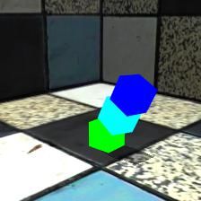
working memory inspired by cognitive science, and such a match can trigger computational actions
that update working memory or external actions that operate on the outside world.
Production systems were typically used to model high-level cognition, e.g., mathematical problem
solving or procedure following; perception was not the focus of these models. It was assumed
that the results of perception were placed into working memory in a symbolic form that could be
operated on with the rules. In this article, we revisit production systems but from a deep learning
perspective which naturally integrates perceptual processing and subsequent inference for visual
reasoning problems. We describe an end-to-end deep learning model that constructs object-centric
representations of entities in videos, and then operates on these entities with differentiable—and
thus learnable—production rules. The essence of these rules, carried over from traditional symbolic
system, is that they operate on variables that are bound, or linked, to the entities in the world. In the
deep learning implementation, each production rule is represented by a distinct MLP with query-key
attention mechanisms to specify the rule-entity binding and to determine when the rule should be
triggered for a given entity.
1.1 Variables and entities
What makes a rule general-purpose is that it
incorporates placeholder variables that can be
bound to arbitrary values or—the term we pre-
fer in this article—entities. This notion of bind-
ing is familiar in functional programming lan-
guages, where these variables are called argu-
ments. Analogously, the use of variables in the Rule 1 Rule 2
production rules we describe enable a model to 0.84 0.16
reason about any set of entities that satisfy the
0.62 0.38
selection criteria of the rule.
0.29 0.71
In order for rules to operate on entities, these
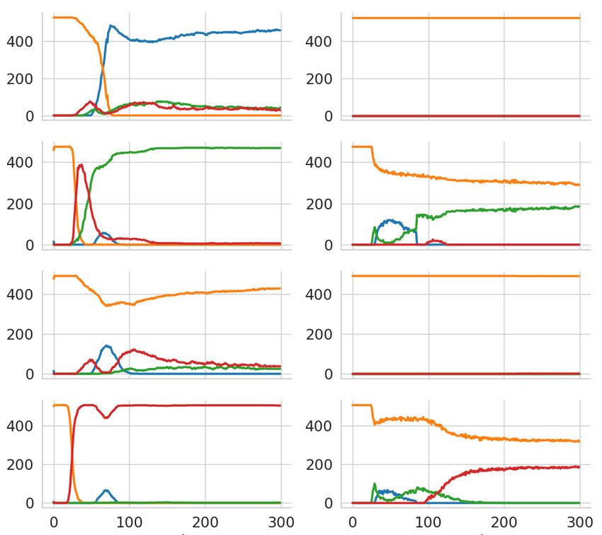
entities must be represented explicitly. That is, Figure 1: Here we show the rule selection statis-
the visual world needs to be parsed in a task- tics from the proposed model for all entities in the
relevant manner, e.g., distinguishing the sprites shapes stack dataset across all examples. Each ex-
in a video game or the vehicles and pedestrians ample contains 3 entities as shown above. Each
approaching an autonomous vehicle. Only in cell in the table shows the probability with which
the past few years have deep learning vision re- the given rule is triggered for the corresponding
searchers developed methods for object-centric entity. We can see that the bottom-most entity
representation (Le Roux et al., 2011; Eslami triggers rule 2 most of the time while the other 2
et al., 2016; Greff et al., 2016; Raposo et al., entities trigger rule 1 most often. This is quite intu-
2017; Van Steenkiste et al., 2018; Kosiorek itive as, for most examples, the bottom-most entity
et al., 2018; Engelcke et al., 2019; Burgess et al., remains static and does not move at all while the
2019; Greff et al., 2019; Locatello et al., 2020a; upper entities fall. Therefore, rule 2 captures in-
Ahmed et al., 2020; Goyal et al., 2019b; Zablot- formation which is relevant to static entities, while
skaia et al., 2020; Rahaman et al., 2020; Du rule 1 captures physical rules relevant to the inter-
et al., 2020; Ding et al., 2020; Goyal et al., 2020; actions and motion of the upper entities.
Ke et al., 2021). These methods differ in details
but share the notion of a fixed number of slots, also known as object files, each encapsulating informa-
tion about a single object. Importantly, the slots are interchangeable, meaning that it doesn’t matter if
a scene with an apple and an orange encodes the apple in slot 1 and orange in slot 2 or vice-versa.
A model of visual reasoning must not only be able to represent entities but must also express
knowledge about entity dynamics and interactions. To ensure systematic predictions, a model must
be capable of applying knowledge to an entity regardless of the slot it is in and must be capable of
applying the same knowledge to multiple instances of an entity. Several distinct approaches exist in
the literature. The predominant approach uses graph neural networks to model slot-to-slot interactions
(Scarselli et al., 2008; Bronstein et al., 2017; Watters et al., 2017; Van Steenkiste et al., 2018; Kipf
et al., 2018; Battaglia et al., 2018; Tacchetti et al., 2018). To ensure systematicity, the GNN must
share parameters among the edges. In a recent article, Goyal et al. (2020) developed a more general
framework in which parameters are shared but slots can dynamically select which parameters to use in
a state-dependent manner. Each set of parameters is referred to as a schema, and slots use a query-key
attention mechanism to select which schema to apply at each time step. Multiple slots can select the
same schema. In both GNNs and SCOFF, modeling dynamics involves each slot interacting with
2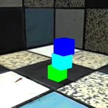
each other slot. In the work we describe in this article, we replace the direct slot-to-slot interactions
with rules, which mediate sparse interactions among slots.
Through our experiments, we show that factorization of knowledge into rules provides a strong
inductive bias for learning interaction dynamics among entities in rich physical environments. Rep-
resenting entity dynamics using NPS leads to impressive performance gains over commonly used
models such as GNNs in a wide variety of physical environments. We also find that the distinct rules
learned by the proposed model are quite intuitive and interpretable as shown in Figure 1. The figure
shows rule selection statistics of the proposed Neural Production System model for the shapes stack
dataset (Groth et al., 2018) when using 2 rules. The shapes stack dataset consists of 3 entities that
are stacked into a tower and fall under the influence of gravity. In the next section, we describe the
proposed model that learns neural representations of entities and rules.
2    Production System
Formally, our notion of a production system consists of a set of entities and a set of rules, along
with a mechanism for selecting rules to apply on subsets of the entities. Implicit in a rule is a
specification of the properties of relevant entities, e.g., a rule might apply to one type of sprite in a
video game but not another. The control flow of a production system dynamically selects rules as
well as bindings between rules and entities, allowing different rules to be chosen and different entities
to be manipulated at each point in time.
The neural production system we describe shares essential properties with traditional production
system, particularly with regard to the compositionality and generality of the knowledge they embody.
Lovett & Anderson (2005) describe four desirable properties commonly attributed to symbolic
systems that apply to our work as well.
Production rules are modular. Each production rule represents a unit of knowledge and are atomic
such that any production rule can be intervened (added, modified or deleted) independently of other
production rules in the system.
Production rules are abstract. Production rules allow for generalization because their conditions
may be represented as high-level abstract knowledge that match to a wide range of patterns. These
conditions specify the attributes of relationship(s) between entities without specifying the entities
themselves. The ability to represent abstract knowledge allows for the transfer of learning across
different environments as long as they fit within the conditions of the given production rule.
Production rules are sparse. In order that production rules have broad applicability, they involve
only a subset of entities. This assumption imposes a strong prior that dependencies among entities
are sparse. In the context of visual reasoning, we conjecture that this prior is superior to what has
often been assumed in the past, particularly in the disentanglement literature—independence among
entities Higgins et al. (2016); Chen et al. (2018).
Production rules represent causal knowledge and are thus asymmetric. Each rule can be decomposed
into a {condition, action} pair, where the action reflects a state change that is a causal consequence of
the conditions being met.
These four properties are sufficient conditions for knowledge to be expressed in production rule form.
These properties specify how knowledge is represented, but not what knowledge is represented. The
latter is inferred by learning mechanisms under the inductive bias provided by the form of production
rules.
3    Neural Production System: Slots and Sparse Rules
The Neural Production System (NPS), illustrated in Figure 2, provides an architectural backbone
that supports the detection and inference of entity (object) representations in an input sequence, and
the underlying rules which govern the interactions between these entities in time and space. The
input sequence indexed by time step t, {x1 , . . . , xt , . . . , xT }, for instance the frames in a video, are
processed by a neural encoder (Burgess et al., 2019; Greff et al., 2019; Goyal et al., 2019b, 2020)
applied to each xt , to obtain a set of M entity representations {V1t , . . . , . . . , VM t
                                                                                             }, one for each of
the M slots. These representations describe an entity and are updated based on both the previous
state, V t−1 and the current input, xt .
NPS consists of N separately encoded rules, {R1 , R2 , .., RN }. Each rule consists of two compo-
             ~ i , M LPi ), where R
nents, Ri = (R                    ~ i is a learned rule embedding vector, which can be thought of as

                                                      3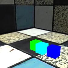
a template defining the condition for when a rule applies; and M LPi , which determines the action
                      ~ i and the parameters of M LPi are learned along with the other parameters of
taken by a rule. Both R
the model using back-propagation on an objective optimized end-to-end.
                                                                                                        RuleN
In the general form of the model, each slot se-

                                                                                                        …
                                                                      slot4
                                                                                                              Rule2
                                                                                                                Rule1
lects a rule that will be applied to it to change its
state. This can potentially be performed several

                                                                      slot3
times, with possibly different rules applied at

                                                                      slot2
each step. Rule selection is done using an atten-
tion mechanism described in detail below. Each

                                                                      slot1
rule specifies conditions and actions on a pair
of slots. Therefore, while modifying the state                                slot1   slot2   slot3   slot4

of a slot using a rule, it can take the state of an-
other slot into account. The slot which is being        Figure 2:       Rule and slot combinatorics.
modified is called the primary slot and other is        Condition-action rules specify how entities inter-
called the contextual slot. The contextual slot         act. Slots maintain the time-varying state of an
is also selected using an attention mechanism           entity. Every rule is matched to every pair of slots.
described in detail below.                              Through key-value attention, a goodness of match
                                                        is determined, and a rule is selected along with its
3.1 Computational Steps in NPS                          binding to slots.
In this section, we give a detailed description of
the rule selection and application procedure for
the slots. First, we will formalize the definitions of a few terms that we will use to explain our method.
We use the term primary slot to refer to slot Vp whose state gets modified by a rule Rr . We use the
term contextual slot to refer to the slot Vc that the rule Rr takes into account while modifying the
state of the primary slot Vp .
Notation. We consider a set of N rules {R1 , R2 , . . . , RN } and a set of T input frames
{x1 , x2 , . . . , xT }. Each frame xt is encoded into a set of M slots {V1t , V2t , . . . , VM
                                                                                              t
                                                                                                }. In the
following discussion, we omit the index over t for simplicity.
Step 1. is external to NPS and involves parsing an input image, xt , into slot-based entities conditioned
on the previous state of the slot-based entities. Any of the methods proposed in the literature to obtain
a slot-wise representation of entities can be used (Burgess et al., 2019; Greff et al., 2019; Goyal et al.,
2019b, 2020). The next three steps constitute the rule selection and application procedure.
Step 2. For each primary slot Vp , we attend to a rule Rr to be applied. Here, the queries come from
the primary slot: qp = Vp W q , and the keys come from the rules: ki = Ri W k ∀i ∈ {1, . . . , N }.
The rule is selected using a straight-through Gumbel softmax (Jang et al., 2016) to achieve a learnable
hard decision: r = argmaxi (qp ki + γ), where γ ∼ Gumbel(0, 1). This competition is a noisy
version of rule matching and prioritization in traditional production systems.
Step 3. For a given primary slot Vp and selected rule Rr , a contextual slot Vc is selected using another
attention mechanism. In this case the query comes from the primary slot: qp = Vp W q , and the
keys from all the slots: kj = Vj W q ∀j ∈ {1, . . . , M }. The selection takes place using a straight-
through Gumbel softmax similar to step 2: c = argmaxj (qp kj + γ), where γ ∼ Gumbel(0, 1).
Note that each rule application is sparse since it takes into account only 1 contextual slot for modifying
a primary slot, while other methods like GNNs take into account all slots for modifying a primary
slot.
Step 4. Rule Application: the selected rule Rr is applied to the primary slot Vp based on the rule and
the current contents of the primary and contextual slots. The rule-specific M LPr , takes as input the
concatenated representation of the state of the primary and contextual slots, Vp and Vc , and produces
an output, which is then used to change the state of the primary slot Vp by residual addition.
3.2 Rule Application: Sequential vs Parallel Rule Application
In the previous section, we have described how each rule application only considers another contextual
slot for the given primary slot i.e., contextual sparsity. We can also consider application sparsity,
wherein we use the rules to update the states of only a subset of the slots. In this scenario, only
the selected slots would be primary slots. This setting will be helpful when there is an entity in an
environment that is stationary, or it is following its own default dynamics unaffected by other entities.
Therefore, it does not need to consider other entities to update its state. We explore two scenarios for
enabling application sparsity.

                                                        4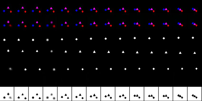
Rules

                                                                                               State Change
Parallel Rule Application. Each of the M slots                                                 No State Change
selects a rule to potentially change its state. To                     Sequential                        Parallel

enable sparse changes, we provide an extra Null
Rule in addition to the available N rules. If a
slot picks the null rule in step 2 of the above           Slots                             Slots

procedure, we do not update its state.
Sequential Rule Application. In this setting,
only one slot gets updated in each rule applica-
                                                    Figure 3: This figure demonstrates the sequential
tion step. Therefore, only one slot is selected
                                                    and parallel rule application.
as the primary slot. This can be facilitated by
modifying step 2 above to select one {primary slot, rule} pair among N M {rule, slot} pairs. The
queries come from each slot: qj = Vj W q ∀j ∈ {1, . . . , M }, the keys come from the rules:
ki = Ri W k ∀i ∈ {1, . . . , N }. The straight-through Gumbel softmax selects one (primary slot,
rule) pair: p, r = argmaxi,j (qp ki + γ), where γ ∼ Gumbel(0, 1). In the sequential regime, we
allow the rule application procedure (step 2, 3, 4 above) to be performed multiple times iteratively in
K rule application stages for each time-step t.
A pictorial demonstration of both rule application regimes can be found in Figure 3. We provide
detailed algorithms for the sequential and parallel regimes in Appendix.

4   Related Work
Key-Value Attention. Key-value attention (Bahdanau et al., 2014) defines the backbone of updates
to the slots in the proposed model. This form of attention is widely used in Transformer models
(Vaswani et al., 2017). Key-value attention selects an input value based on the match of a query
vector to a key vector associated with each value. To allow easier learnability, selection is soft and
computes a convex combination of all the values. Rather than only computing the attention once, the
multi-head dot product attention mechanism (MHDPA) runs through the scaled dot-product attention
multiple times in parallel. There is an important difference with NPS: in MHDPA, one can treat
different heads as different rule applications. Each head (or rule) considers all the other entities as
relevant arguments as compared to the sparse selection of arguments in NPS.
Sparse and Dense Interactions. GNNs model pairwise interactions between all the slots hence they
can be seen as capturing dense interactions (Scarselli et al., 2008; Bronstein et al., 2017; Watters
et al., 2017; Van Steenkiste et al., 2018; Kipf et al., 2018; Battaglia et al., 2018; Tacchetti et al., 2018).
Instead, verbalizable interactions in the real world are sparse (Bengio, 2017): the immediate effect
of an action is only on a small subset of entities. In NPS, a selected rule only updates the state of a
subset of the slots.
In NPS, one can view the computational graph as a dynamically constructed GNN resulting from
applying dynamically selected rules, where the states of the slots are represented on the different
nodes of the graph, and different rules dynamically instantiate an hyper-edge between a set of slots
(the primary slot and the contextual slot). It is important to emphasize that the topology of the graph
induced in NPS is dynamic, while in most GNNs the topology is fixed. Through a thorough set
of experiments, we show that learning sparse and dynamic interactions using NPS indeed works
better for the problems we consider than learning dense interactions using GNNs. We show that NPS
outperforms state-of-the-art GNN-based architectures such as C-SWM Kipf et al. (2019) and OP3
Veerapaneni et al. (2019) while learning action conditioned world models.

5   Experiments
We demonstrate the effectiveness of NPS on multiple tasks and compare to a comprehensive set of
baselines. To show that NPS can learn intuitive rules from the data generating distribution, we design
a couple of simple toy experiments with well-defined discrete operations. Results show that NPS
can accurately recover each operation defined by the data and learn to represent each operation using
a separate rule. We then move to a much more complicated and visually rich setting with abstract
physical rules and show that factorization of knowledge into rules as offered by NPS does scale up to
such settings. We study and comparison the parallel and sequential rule application procedures and
try to understand the settings which favour each. We then evaluate the benefits of reusable, dynamic
and sparse interactions as offered by NPS in a wide variety of physical environments by comparing
it against baselines with dense interactions like GNNs. We conduct ablation studies to assess the

                                                      5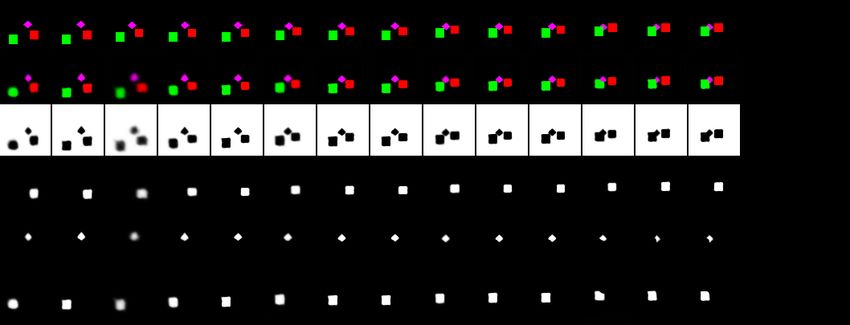
contribution of different components of NPS. Here we briefly outline the tasks considered and direct
the reader to the Appendix for full details on each task and details on hyperparameter settings.

5.1   Learning intuitive rules with NPS: Toy Simulations

We designed a couple of simple tasks with well-defined                      Table 1: This table shows the segrega-
discrete rules to show that NPS can learn intuitive and                     tion of rules for the MNIST Transforma-
interpretable rules. We also show the efficiency and effec-                 tion task. Each cell indicates the number
tiveness of the selection procedure (step 2 and step 3 in                   of times the corresponding rule is used
section 3.1) by comparing against a baseline with many                      for the given operation. We can see that
more parameters. Both tasks require a single modification                   NPS automatically and perfectly learns
of only one of the available entities, therefore the use of                 a separate rule for each operation.
sequential or parallel rule application would not make a
                                                                                              Rule 1 Rule 2 Rule 3 Rule 4
difference here since parallel rule application in which all-                  Translate Down 5039     0      0      0
but-one slots select the null rule is similar to sequential rule                Translate Up    0    4950     0      0
application with 1 rule application step. To simplify the                       Rotate Right    0      0    5030     0
                                                                                 Rotate Left    0      0      0    4981
presentation, we describe the setup for both tasks using the
sequential rule application procedure.
MNIST Transformation. We test whether NPS can learn simple rules for performing transforma-
tions on MNIST digits. We generate data with four transformations: {Translate Up, Translate Down,
Rotate Right, Rotate Left}. We feed the input image (X) and the transformation (o) to be performed
as a one-hot vector to the model. The detailed setup is described in Appendix. For this task, we
evaluate whether NPS can learn to use a unique rule for each transformation.
We use 4 rules corresponding to the 4 transformations with the hope that the correct transformations
are recovered. Indeed, we observe that NPS successfully learns to represent each transformation
using a separate rule as shown in Table 1. Our model achieves an MSE of 0.02. A visualization of
the outputs from our model can be found in Appendix C.
Coordinate Arithmetic Task. The model is                                                    Rule No.
                                                                               Rule 1    Rule 2        Rule 3        Rule 4
to perform arithmetic operations on 2D co-
ordinates. Given (X0 , Y0 ) and (X1 , Y1 ), we                                 NPS                              Baseline

can apply the following operations: {X Ad-

                                                                                                                                 X Addition
                                                                Frequency

dition: (Xr , Yr ) = (X0 + X1 , Y0 ), X Sub-
traction: (Xr , Yr ) = (X0 − X1 , Y0 ), Y Ad-
dition: (Xr , Yr ) = (X0 , Y0 + Y1 ), Y Subtrac-

                                                                                                                                X Subtraction
tion: Xr , Yr = (X0 , Y0 − Y1 )}, where (Xr , Yr )
                                                                Frequency

is the resultant coordinate.
In this task, the model is given 2 input coordi-                                                                              Y Addition

nates X = [(xi , yi ), (xj , yj )] and the expected
                                                                Frequency

output coordinates Y = [(x̂i , yˆi ), (xˆj , yˆj )] . The
model is supposed to infer the correct rule to
produce the correct output. The correct output
                                                                                                                              Y Subtraction
                                                                Frequency

is obtained by performing a randomly selected
transformation on a randomly selected coordi-
nate in X (primary coordinate), taking another
                                                                              Epochs                            Epochs
randomly selected coordinate from X (contex-
tual coordinate) into account. The detailed setup
                                                            Figure 4: Coordinate Arithmetic Task. Here,
is described in Appendix D. We use an NPS
                                                            we compare NPS to the baseline model in terms
model with 4 rules for this task, with the the
                                                            of segregation of rules as the training progresses.
selection procedure in step 2 and step 3 of algo-
                                                            X-axis shows the epochs and Y-axis shows the
rithm 1 to select the primary coordinate, contex-
                                                            frequency with which Rule i is used for the given
tual coordinate, and the rule. For the baseline
                                                            operation. We can see that NPS disentangles the
we replace the selection procedure in NPS (i.e.
                                                            operations perfectly as training progresses with a
step 2 and step 3 in algorithm 1) with a routing
                                                            unique rule specializing to every operation while
MLP similar to Fedus et al. (2021).
                                                            the baseline model fails to do so.
This routing MLP has 3 heads (one each for
selecting the primary coordinate, contextual coordinate, and the rule). The baseline has 4 times more
parameters than NPS. The final output is produced by the rule MLP which does not have access

                                                            6
to the correct output, hence the model cannot simply copy the correct output to produce the actual
output. Unlike the MNIST transformation task, we do not provide the operation to be performed as a
one-hot vector input to the model, therefore it needs to infer the available operations from the data
demonstrations.
We show the segregation of rules for NPS and the baseline Table 2: This table shows segregation
in Figure 4. We can see that NPS learns to use a unique of rules when we use NPS with 5 rules
rule for each operation while the baseline struggles to but the data generation distributions de-
disentangle the underlying operations properly. NPS scribes only 4 possible operations. We
also outperforms the baseline in terms of MSE achiev- can see that only 4 rules get majorly uti-
ing an MSE of 0.01±0.001 while the baseline achieves an lized thus confirming that NPS success-
MSE of 0.04±0.008 . To further confirm that NPS learns all fully recovers all possible operations de-
the available operations correctly from raw data demon- scribed by the data.
strations, we use an NPS model with 5 rules. We expect
Rule 1 Rule 2 Rule 3 Rule 4 Rule 5
that in this case NPS should utilize only 4 rules since
X Addition 360 99 45 13 0
the data describes only 4 unique operations and indeed
X Subtraction 0 482 0 1 0
we observe that NPS ends up mostly utilizing 4 of the Y Subtraction 0 39 453 2 0
available 5 rules as shown in Table 2. Y Addition 0 57 15 99 335
5.2 Parallel vs Sequential Rule Application
We compare the parallel and sequential rule application procedures, to understand the settings that
favour one or the other, over two tasks: (1) Bouncing Balls, (2) Shapes Stack. We use the term PNPS
to refer to parallel rule application and SNPS to refer to sequential rule application.
Shapes Stack. We use the shapes stack dataset introduced by Groth et al. (2018). This dataset
consists of objects stacked on top of each other as shown in Figure 1. These objects fall under the
influence of gravity. For our experiments, We follow the same setup as Qi et al. (2021). In this
task, given the first frame, the model is tasked with predicting the object bounding boxes for the
next t timesteps. The first frame is encoded using a convolutional network followed by RoIPooling
(Girshick (2015)) to extract object-centric visual features. The object-centric features are then passed
to the dynamics model to the predict object bounding boxes of the next t steps. Qi et al. (2021)
propose a Region Proposal Interaction Network (RPIN) to solve this task. The dynamics model in
RPIN consists of an Interaction Network proposed in Battaglia et al. (2016). To better utilize spatial
information, Qi et al. (2021) propose an extension of the interaction operators in interaction net to
operate on 3D tensors. This is achieved by replacing the MLP operations in the original interaction
networks with convolutions. They call this new network Convolutional Interaction Network (CIN).
For the proposed model, we replace this CIN by NPS. To ensure a fair comparison to CIN, we use
CNNs to represent rules in NPS instead of MLPs. CIN captures all pairwise interactions between
objects using a convolutional network. In NPS, we capture sparse interactions (contextual sparsity) as
compared to dense pairwise interactions captured by CIN. Also, in NPS we update only a few subset
of slots per step instead of all slots (application sparsity).
We consider two evaluation settings. (1) Test setting: The number of rollout timesteps is same as that
seen during training (i.e. t = 15); (2) Transfer Setting: The number of rollout timesteps is higher
than that seen during training (i.e. t = 30).
We present our results on the shapes stack dataset in Table Model Name Test Transfer
3. We can see that both PNPS and SNPS outperform the RPIN (Qi et al. (2021)) 1.24±0.01 6.12±0.22
baseline RPIN in the transfer setting, while only PNPS PNPS 1.23±0.01 5.22±0.52
outperforms the baseline in the test setting and SNPS fails SNPS 1.68±0.02 5.80±0.15
to do so. We can see that PNPS outperforms SNPS. We at-
Table 3: Prediction error of the com-
tribute this to the reduced application sparsity with PNPS,
pared models on the shapes stack
i.e., it is more likely that the state of a slot gets updated
in PNPS as compared to SNPS. For instance, consider an dataset (lower is better) for the test as
NPS model with N uniformly chosen rules and M slots. well as transfer setting. In the test set-
ting the number of rollout steps t is set
The probability that the state of a slot gets updated in PNPS
is PP N P S = N −1/N (since 1 rule is the null rule), while
to 15 and in the transfer setting it is set
the same probability for SNPS is PSN P S = 1/M (since to 30. We can see that PNPS outper-
only 1 slot gets updated per rule application step). forms the RPIN baseline in both the test
and transfer setting while SNPS fails to
For this task, we run both PNPS and SNPS for N =
do so.
{1, 2, 4, 6} rules and M = 3. For any given N , we can
7see that PP N P S > PSN P S . Even when we have multiple rule application steps in SNPS, it might
end up selecting the same slot to be updated in more than one of these steps. We report the best
performance obtained for PNPS and SNPS across all N , which is N = {2 + 1 Null Rule} for
PNPS and N = 4 for SNPS, in Table 3. Shapes stack is a dataset that would prefer a model with
less application sparsity since all the objects are tightly bound to each other (objects are placed on
top of each other), therefore all objects spend the majority of their time interacting with the objects
directly above or below them. We attribute the higher performance of PNPS compared to RPIN to
the higher contextual sparsity of PNPS. Each example in the shapes stack task consists of 3 objects.
Even though the blocks are tightly bound to each other, each block is only affected by the objects
it is in direct contact with. For example, the top-most object is only affected by the object directly
below it. The contextual sparsity offered by PNPS is a strong inductive bias to model such sparse
interactions while RPIN models all pairwise interactions between the objects. Figure 1 shows an
illustration of the PNPS model for the shapes stack dataset. In the figure, Rule 2 actually refers to the
Null Rule, while Rule 1 refers to all the other non-null rules. The bottom-most block picks the Null
Rule most times, as the bottom-most block generally does not move.
Bouncing Balls. We consider a bouncing-balls environ-
ment in which multiple balls move with billiard-ball dy- Model Name Test Transfer
namics. We validate our model on a colored version of this SCOFF 0.28 0.15
dataset. This is a next-step prediction task in which the SCOFF++ 0.8437 0.2632
model is tasked with predicting the final binary mask of PNPS (10 Rules+1 Null Rule) 0.7813 0.1997
each ball. We compare the following methods: (a) SCOFF SNPS (10 Rules) 0.8518 0.3553
(Goyal et al., 2020): factorization of knowledge in terms
of slots (object properties) and schemata, the latter captur- Table 4: Here we show the ARI
ing object dynamics; (b) SCOFF++: we extend SCOFF achieved by the models on the bouncing
by using the idea of iterative competition as proposed in balls dataset (higher is better). We can
slot attention (SA) (Locatello et al., 2020a); SCOFF + see that SNPS outperforms SCOFF and
PNPS/SNPS: We replace pairwise slot-to-slot interaction SCOFF++ while PNPS has a poor per-
in SCOFF++ with parallel or sequential rule application. formance in this task. Results average
For comparing different methods, we use the Adjusted across 2 seeds.
Rand Index or ARI (Rand, 1971). To investigate how the factorization in the form of rules allows
for extrapolating knowledge from fewer to more objects, we increase the number of objects from 4
during training to 6-8 during testing.
We present the results of our experiments in Table 4. Contrary to the shapes stack task, we see
that SNPS outperforms PNPS for the bouncing balls task. The balls are not tightly bound together
into a single tower as in the shapes stack. Most of the time, a single ball follows its own dynamics,
only occasionally interacting with another ball. Rules in NPS capture interaction dynamics between
entities, hence they would only be required to change the state of an entity when it interacts with
another entity. In the case of bouncing balls, this interaction takes place through a collision between
multiple balls. Since for a single ball, such collisions are rare, SNPS, which has higher application
sparsity (less probability of modifying the state of an entity), performs better as compared to PNPS
(lower application sparsity). Also note that, SNPS has the ability to compose multiple rules together
by virtue of having multiple rule application stages.
Given the analysis in this section, we can conclude that PNPS is expected to work better when
interactions among entities are more frequent while SNPS is expected to work better when interactions
are rare and most of the time, each entity follows its own dynamics. Note that, for both SNPS and
PNPS, the rule application considers only 1 other entity as context. Therefore, both approaches have
equal contextual sparsity while the baselines that we consider (SCOFF and RPIN) capture dense
pairwise interactions. We discuss the benefits of contextual sparsity in more detail in the next section.
More details regarding our setup for the above experiments can be found in Appendix.
5.3 Benefits of Sparse Interactions Offered by NPS
In this section, we compare NPS to GNNs across a wide variety of physical settings. GNNs offer
dense pairwise interactions and modify the state of each of the entities at every step while NPS
modifies the state of only a subset of entities per step and uses only one other entity as context while
modifying the state of an entity. In this section, we consider two types of tasks: (1) Learning Action
Conditioned World Models (2) Physical Reasoning. We use SNPS for all these experiments since in
the environments that we consider here, interactions among entities are rare.
8Learning Action-Conditioned World Models. Here, we present empirical results to support
the discussion in section 4. For learning action-conditioned world models, we follow the same
experimental setup as Kipf et al. (2019). Therefore, all the tasks in this section are next-K step
(K = {1, 5, 10}) prediction tasks, given the intermediate actions, and with the predictions being
performed in the latent space. We use the Hits at Rank 1 (H@1) metrics described by Kipf et al.
(2019) for evaluation. H@1 is 1 for a particular example if the predicted state representation is nearest
to the encoded true observation and 0 otherwise. We report the average of this score over the test set
(higher is better).
Physics Environment. The physics environment (Ke et al., 2021) simulates a simple physical
world. It consists of blocks of unique but unknown weights. The dynamics for the interaction between
blocks is that the movement of heavier blocks pushes lighter blocks on their path. This rule creates an
acyclic causal graph between the blocks. For an accurate world model, the learner needs to infer the
correct weights through demonstrations. Interactions in this environment are sparse and only involve
two blocks at a time, therefore we expect NPS to outperform dense architectures like GNNs. This
environment is demonstrated in Appendix Fig 9.
We follow the same setup as Kipf et al. (2019). We use their C-SWM model as baseline. For the
proposed model, we only replace the GNN from C-SWM by NPS. GNNs generally share parameters
across edges, but in NPS each rule has separate parameters. For a fair comparison to GNN, we use
an NPS model with 1 rule. Note that this setting is still different from GNNs as in GNNs at each
step every slot is updated by instantiating edges between all pairs of slots, while in NPS an edge is
dynamically instantiated between a single pair of slots and only the state of the selected slot (i.e.,
primary slot) gets updated.
Model Model
80 NPS 40 NPS
GNN GNN
70 35
60 30
50 25
H@1
H@1
40 20
30 15
20 10
10 5
0 0
1 5 10 1 5 10
Steps Steps
(a) Physics Env (b) Atari Games
Figure 5: Action-Conditioned World Models, with number of future steps to be predicted for the
world-model on the horizontal axes. (a) Here we show a comparison between GNNs and the proposed
NPS on the physics environment using the H@1 metric (higher is better). (b) Comparison of average
H@1 scores across 5 Atari games for the proposed model NPS and GNN.
The results of our experiments are presented in Figure 5(a). We can see that NPS outperforms
GNNs for all rollouts. Multi-step settings are more difficult to model as errors may get compounded
over time steps. The sparsity of NPS (only a single slot affected per step) reduces compounding of
errors and enhances symmetry-breaking in the assignment of transformations to rules, while in the
case of GNNs, since all entities are affected per step, there is a higher possibility of errors getting
compounded. We can see that even with a single rule, we significantly outperform GNNs thus proving
the effectiveness of dynamically instantiating edges between entities.
Atari Games. We also test the proposed model in the more complicated setting of Atari. Atari
games also have sparse interactions between entities. For instance, in Pong, any interaction involves
only 2 entities: (1) paddle and ball or (2) ball and the wall. Therefore, we expect sparse interactions
captured by NPS to outperform GNNs here as well.
We follow the same setup as for the physics environment described in the previous section. We
present the results for the Atari experiments in Figure 5(b), showing the average H@1 score across
5 games: Pong, Space Invaders, Freeway, Breakout, and QBert. As expected, we can see that the
proposed model achieves a higher score than the GNN-based C-SWM. The results for the Atari
experiments reinforce the claim that NPS is especially good at learning sparse interactions.
Learning Rules for Physical Reasoning. To show the effectiveness of the proposed approach for
physical reasoning tasks, we evaluate NPS on another dataset: Sprites-MOT (He et al., 2018). The
9Model MOTA ↑ MOTP ↑ Mostly Detected ↑ Mostly Tracked ↑ Match ↑ Miss ↓ ID Switches ↓ False Positives ↓
OP3 89.1±5.1 78.4±2.4 92.4±4.0 91.8±3.8 95.9±2.2 3.7±2.2 0.4±0.0 6.8±2.9
NPS 90.72±5.15 79.91±0.1 94.66±0.29 93.18±0.84 96.93±0.16 2.48±0.07 0.58±0.02 6.2±3.5
Table 5: Sprites-MOT. Comparison between the proposed NPS and the baseline OP3 for various
MOT (multi-object tracking) metrics on the sprites-MOT dataset (↑: higher is better, ↓: lower is
better). Average over 3 random seeds.
Sprites-MOT dataset was introduced by He et al. (2018). The dataset contains a set of moving objects
of various shapes. This dataset aims to test whether a model can handle occlusions correctly. Each
frame has consistent bounding boxes which may cause the objects to appear or disappear from the
scene. A model which performs well should be able to track the motion of all objects irrespective
of whether they are occluded or not. We follow the same setup as Weis et al. (2020). We use the
OP3 model (Veerapaneni et al., 2019) as our baseline. To test the proposed model, we replace the
GNN-based transition model in OP3 with the proposed NPS.
We use the same evaluation protocol as followed by Weis et al. (2020) which is based on the MOT
(Multi-object tracking) challenge (Milan et al., 2016). The results for this task are presented in Table
5. We ask the reader to refer to appendix F.1 for more details. We can see that for almost all metrics,
NPS outperforms the OP3 baseline. Although this dataset does not contain physical interactions
between the objects, sparse rule application should still be useful in dealing with occlusions. At
any time step, only a single object is affected by occlusions i.e., it may get occluded due to another
object or due to a prespecified bounding box, while the other objects follow their default dynamics.
Therefore, a rule should be applied to only the object (or entity) affected (i.e., not visible) due to
occlusion and may take into account any other object or entity that is responsible for the occlusion.
6 Discussion and Conclusion
Looking Backward. Production systems were one of the first AI research attempts to model cognitive
behaviour and form the basis of many existing models of cognition. However, in traditional symbolic
AI, both the key entities and the rules that operated on the entities were given. For AI agents such as
robots trying to make sense of their environment, the only observables are low-level variables like
pixels in images. To generalize well, an agent must induce high-level entities as well as discover and
disentangle the rules that govern how these entities actually interact with each other. Here we have
focused on perceptual inference problems and proposed NPS, a neural instantiation of production
systems by introducing an important inductive bias in the architecture following the proposals of
Bengio (2017); Goyal & Bengio (2020); Ke et al. (2021).
Limitations & Looking Forward. Our experiments on learning action-conditioned world models
and extrapolation of knowledge in the form of learned rules in video prediction highlight the advan-
tages brought by the factorization of knowledge into a small set of entities and sparse sequentially
applied rules. Immediate future work would investigate how to take advantage of these inductive
biases for more complex physical environments (Ahmed et al., 2020) and novel planning methods,
which might be more sample efficient than standard ones (Schrittwieser et al., 2020). Humans seem to
exploit the inductive bias in the sparsity of the rules and that reasoning about the application of these
rules in an abstract space can be very efficient.For such problems, exploration becomes a bottleneck
but we believe using rules as a source of behavioural priors can drive the necessary exploration
(Goyal et al., 2019a; Tirumala et al., 2020; Badia et al., 2020).
Social Impact. The authors do not foresee negative social impact of this work beyond that which
could arise from general improvements in ML.
7 Acknowledgements
The authors would like to thank Matthew Botvinick for useful discussions. The authors would also
like to thank Alex Lamb, Stefan Bauer, Nicolas Chapados, Danilo Rezende and Kelsey Allen for
brainstorming sessions. We are also thankful to Dianbo Liu, Damjan Kalajdzievski and Osama
Ahmed for proofreading.
10References
Ahmed, O., Träuble, F., Goyal, A., Neitz, A., Wüthrich, M., Bengio, Y., Schölkopf, B., and Bauer, S.
Causalworld: A robotic manipulation benchmark for causal structure and transfer learning. arXiv
preprint arXiv:2010.04296, 2020.
Anderson, J. R. Skill acquisition: Compilation of weak-method problem situations. Psychological
review, 94(2):192, 1987.
Andreas, J., Rohrbach, M., Darrell, T., and Klein, D. Neural module networks. In Proceedings of the
IEEE Conference on Computer Vision and Pattern Recognition, pp. 39–48, 2016.
Badia, A. P., Piot, B., Kapturowski, S., Sprechmann, P., Vitvitskyi, A., Guo, Z. D., and Blundell, C.
Agent57: Outperforming the atari human benchmark. In International Conference on Machine
Learning, pp. 507–517. PMLR, 2020.
Bahdanau, D., Cho, K., and Bengio, Y. Neural machine translation by jointly learning to align and
translate. arXiv preprint arXiv:1409.0473, 2014.
Battaglia, P. W., Pascanu, R., Lai, M., Rezende, D. J., and Kavukcuoglu, K. Interaction networks
for learning about objects, relations and physics. CoRR, abs/1612.00222, 2016. URL http:
//arxiv.org/abs/1612.00222.
Battaglia, P. W., Hamrick, J. B., Bapst, V., Sanchez-Gonzalez, A., Zambaldi, V., Malinowski, M.,
Tacchetti, A., Raposo, D., Santoro, A., Faulkner, R., et al. Relational inductive biases, deep
learning, and graph networks. arXiv preprint arXiv:1806.01261, 2018.
Bengio, Y. The consciousness prior. arXiv preprint arXiv:1709.08568, 2017.
Bottou, L. and Gallinari, P. A framework for the cooperation of learning algorithms. In Advances in
neural information processing systems, pp. 781–788, 1991.
Bronstein, M. M., Bruna, J., LeCun, Y., Szlam, A., and Vandergheynst, P. Geometric deep learning:
going beyond euclidean data. IEEE Signal Processing Magazine, 34(4):18–42, 2017.
Bunel, R., Hausknecht, M., Devlin, J., Singh, R., and Kohli, P. Leveraging grammar and reinforcement
learning for neural program synthesis. arXiv preprint arXiv:1805.04276, 2018.
Burgess, C. P., Matthey, L., Watters, N., Kabra, R., Higgins, I., Botvinick, M., and Lerchner, A.
Monet: Unsupervised scene decomposition and representation. arXiv preprint arXiv:1901.11390,
2019.
Cai, J., Shin, R., and Song, D. Making neural programming architectures generalize via recursion.
arXiv preprint arXiv:1704.06611, 2017.
Chen, R. T., Li, X., Grosse, R., and Duvenaud, D. Isolating sources of disentanglement in variational
autoencoders. arXiv preprint arXiv:1802.04942, 2018.
Ding, D., Hill, F., Santoro, A., and Botvinick, M. Object-based attention for spatio-temporal
reasoning: Outperforming neuro-symbolic models with flexible distributed architectures. arXiv
preprint arXiv:2012.08508, 2020.
Du, Y., Smith, K., Ulman, T., Tenenbaum, J., and Wu, J. Unsupervised discovery of 3d physical
objects from video. arXiv preprint arXiv:2007.12348, 2020.
Engelcke, M., Kosiorek, A. R., Jones, O. P., and Posner, I. Genesis: Generative scene inference and
sampling with object-centric latent representations. arXiv preprint arXiv:1907.13052, 2019.
Eslami, S., Heess, N., Weber, T., Tassa, Y., Szepesvari, D., Kavukcuoglu, K., and Hinton, G. E. Attend,
infer, repeat: Fast scene understanding with generative models. arXiv preprint arXiv:1603.08575,
2016.
Evans, R., Hernández-Orallo, J., Welbl, J., Kohli, P., and Sergot, M. Making sense of sensory input.
Artificial Intelligence, pp. 103438, 2019.
11Fedus, W., Zoph, B., and Shazeer, N. Switch transformers: Scaling to trillion parameter models with
simple and efficient sparsity. CoRR, abs/2101.03961, 2021. URL https://arxiv.org/abs/
2101.03961.
Fernando, C., Banarse, D., Blundell, C., Zwols, Y., Ha, D., Rusu, A. A., Pritzel, A., and Wierstra,
D. Pathnet: Evolution channels gradient descent in super neural networks. arXiv preprint
arXiv:1701.08734, 2017.
Girshick, R. B. Fast R-CNN. CoRR, abs/1504.08083, 2015. URL http://arxiv.org/abs/1504.
08083.
Goyal, A. and Bengio, Y. Inductive biases for deep learning of higher-level cognition. arXiv preprint
arXiv:2011.15091, 2020.
Goyal, A., Islam, R., Strouse, D., Ahmed, Z., Botvinick, M., Larochelle, H., Levine, S., and Bengio, Y.
Infobot: Transfer and exploration via the information bottleneck. arXiv preprint arXiv:1901.10902,
2019a.
Goyal, A., Lamb, A., Hoffmann, J., Sodhani, S., Levine, S., Bengio, Y., and Schölkopf, B. Recurrent
independent mechanisms, 2019b.
Goyal, A., Lamb, A., Gampa, P., Beaudoin, P., Levine, S., Blundell, C., Bengio, Y., and Mozer, M.
Object files and schemata: Factorizing declarative and procedural knowledge in dynamical systems.
arXiv preprint arXiv:2006.16225, 2020.
Graves, A., Wayne, G., and Danihelka, I. Neural turing machines. arXiv preprint arXiv:1410.5401,
2014.
Greff, K., Rasmus, A., Berglund, M., Hao, T. H., Schmidhuber, J., and Valpola, H. Tagger: Deep
unsupervised perceptual grouping. arXiv preprint arXiv:1606.06724, 2016.
Greff, K., Kaufman, R. L., Kabra, R., Watters, N., Burgess, C., Zoran, D., Matthey, L., Botvinick, M.,
and Lerchner, A. Multi-object representation learning with iterative variational inference. arXiv
preprint arXiv:1903.00450, 2019.
Groth, O., Fuchs, F., Posner, I., and Vedaldi, A. Shapestacks: Learning vision-based physical intuition
for generalised object stacking. CoRR, abs/1804.08018, 2018. URL http://arxiv.org/abs/
1804.08018.
He, Z., Li, J., Liu, D., He, H., and Barber, D. Tracking by animation: Unsupervised learning of
multi-object attentive trackers. CoRR, abs/1809.03137, 2018. URL http://arxiv.org/abs/
1809.03137.
Higgins, I., Matthey, L., Pal, A., Burgess, C., Glorot, X., Botvinick, M., Mohamed, S., and Lerchner,
A. beta-vae: Learning basic visual concepts with a constrained variational framework. 2016.
Jacobs, R. A., Jordan, M. I., Nowlan, S. J., Hinton, G. E., et al. Adaptive mixtures of local experts.
Neural computation, 3(1):79–87, 1991.
Jang, E., Gu, S., and Poole, B. Categorical reparameterization with gumbel-softmax. arXiv preprint
arXiv:1611.01144, 2016.
Ke, N. R., Didolkar, A. R., Mittal, S., Goyal, A., Lajoie, G., Bauer, S., Rezende, D. J., Mozer,
M. C., Bengio, Y., and Pal, C. Systematic evaluation of causal discovery in visual model based
reinforcement learning. 2021.
Kipf, T., Fetaya, E., Wang, K.-C., Welling, M., and Zemel, R. Neural relational inference for
interacting systems. arXiv preprint arXiv:1802.04687, 2018.
Kipf, T., van der Pol, E., and Welling, M. Contrastive learning of structured world models. arXiv
preprint arXiv:1911.12247, 2019.
Kirsch, L., Kunze, J., and Barber, D. Modular networks: Learning to decompose neural computation.
In Advances in Neural Information Processing Systems, pp. 2408–2418, 2018.
12Kosiorek, A., Kim, H., Teh, Y. W., and Posner, I. Sequential attend, infer, repeat: Generative
modelling of moving objects. Advances in Neural Information Processing Systems, 31:8606–8616,
2018.
Laird, J. E., Rosenbloom, P. S., and Newell, A. Chunking in soar: The anatomy of a general learning
mechanism. Machine learning, 1(1):11–46, 1986.
Lamb, A., Goyal, A., Słowik, A., Mozer, M., Beaudoin, P., and Bengio, Y. Neural function modules
with sparse arguments: A dynamic approach to integrating information across layers. arXiv
preprint arXiv:2010.08012, 2020.
Le Roux, N., Heess, N., Shotton, J., and Winn, J. Learning a generative model of images by factoring
appearance and shape. Neural Computation, 23(3):593–650, 2011.
Li, Y., Gimeno, F., Kohli, P., and Vinyals, O. Strong generalization and efficiency in neural programs.
arXiv preprint arXiv:2007.03629, 2020.
Locatello, F., Weissenborn, D., Unterthiner, T., Mahendran, A., Heigold, G., Uszkoreit, J., Dosovitskiy,
A., and Kipf, T. Object-centric learning with slot attention. arXiv preprint arXiv:2006.15055,
2020a.
Locatello, F., Weissenborn, D., Unterthiner, T., Mahendran, A., Heigold, G., Uszkoreit, J., Dosovitskiy,
A., and Kipf, T. Object-centric learning with slot attention, 2020b.
Lovett, M. C. and Anderson, J. R. Thinking as a production system. The Cambridge handbook of
thinking and reasoning, pp. 401–429, 2005.
McMillan, C., Mozer, M. C., and Smolensky, P. The connectionist scientist game: rule extraction and
refinement in a neural network. In Proceedings of the 13th Annual Conference of the Cognitive
Science Society, pp. 424–430, 1991.
Milan, A., Leal-Taixé, L., Reid, I. D., Roth, S., and Schindler, K. MOT16: A benchmark for multi-
object tracking. CoRR, abs/1603.00831, 2016. URL http://arxiv.org/abs/1603.00831.
Neelakantan, A., Le, Q. V., and Sutskever, I. Neural programmer: Inducing latent programs with
gradient descent. arXiv preprint arXiv:1511.04834, 2015.
Qi, H., Wang, X., Pathak, D., Ma, Y., and Malik, J. Learning long-term visual dynamics with region
proposal interaction networks. In International Conference on Learning Representations, 2021.
URL https://openreview.net/forum?id=_X_4Akcd8Re.
Rahaman, N., Goyal, A., Gondal, M. W., Wuthrich, M., Bauer, S., Sharma, Y., Bengio, Y., and
Schölkopf, B. S2rms: Spatially structured recurrent modules. arXiv preprint arXiv:2007.06533,
2020.
Rand, W. M. Objective criteria for the evaluation of clustering methods. Journal of the American
Statistical association, 66(336):846–850, 1971.
Raposo, D., Santoro, A., Barrett, D., Pascanu, R., Lillicrap, T., and Battaglia, P. Discovering objects
and their relations from entangled scene representations. arXiv preprint arXiv:1702.05068, 2017.
Reed, S. and De Freitas, N. Neural programmer-interpreters. arXiv preprint arXiv:1511.06279, 2015.
Ronco, E., Gollee, H., and Gawthrop, P. J. Modular neural networks and self-decomposition.
Technical Report CSC-96012, 1997.
Rosenbaum, C., Klinger, T., and Riemer, M. Routing networks: Adaptive selection of non-linear
functions for multi-task learning. arXiv preprint arXiv:1711.01239, 2017.
Rosenbaum, C., Cases, I., Riemer, M., and Klinger, T. Routing networks and the challenges of
modular and compositional computation. arXiv preprint arXiv:1904.12774, 2019.
Scarselli, F., Gori, M., Tsoi, A. C., Hagenbuchner, M., and Monfardini, G. The graph neural network
model. IEEE Transactions on Neural Networks, 20(1):61–80, 2008.
13Schrittwieser, J., Antonoglou, I., Hubert, T., Simonyan, K., Sifre, L., Schmitt, S., Guez, A., Lockhart,
E., Hassabis, D., Graepel, T., et al. Mastering atari, go, chess and shogi by planning with a learned
model. Nature, 588(7839):604–609, 2020.
Shazeer, N., Mirhoseini, A., Maziarz, K., Davis, A., Le, Q., Hinton, G., and Dean, J. Outra-
geously large neural networks: The sparsely-gated mixture-of-experts layer. arXiv preprint
arXiv:1701.06538, 2017.
Tacchetti, A., Song, H. F., Mediano, P. A., Zambaldi, V., Rabinowitz, N. C., Graepel, T., Botvinick,
M., and Battaglia, P. W. Relational forward models for multi-agent learning. arXiv preprint
arXiv:1809.11044, 2018.
Tirumala, D., Galashov, A., Noh, H., Hasenclever, L., Pascanu, R., Schwarz, J., Desjardins, G.,
Czarnecki, W. M., Ahuja, A., Teh, Y. W., et al. Behavior priors for efficient reinforcement learning.
arXiv preprint arXiv:2010.14274, 2020.
Trask, A., Hill, F., Reed, S. E., Rae, J., Dyer, C., and Blunsom, P. Neural arithmetic logic units. In
Advances in Neural Information Processing Systems, pp. 8035–8044, 2018.
Van Steenkiste, S., Chang, M., Greff, K., and Schmidhuber, J. Relational neural expectation maximiza-
tion: Unsupervised discovery of objects and their interactions. arXiv preprint arXiv:1802.10353,
2018.
Vaswani, A., Shazeer, N., Parmar, N., Uszkoreit, J., Jones, L., Gomez, A. N., Kaiser, L., and
Polosukhin, I. Attention is all you need, 2017.
Veerapaneni, R., Co-Reyes, J. D., Chang, M., Janner, M., Finn, C., Wu, J., Tenenbaum, J. B., and
Levine, S. Entity abstraction in visual model-based reinforcement learning. CoRR, abs/1910.12827,
2019. URL http://arxiv.org/abs/1910.12827.
Veerapaneni, R., Co-Reyes, J. D., Chang, M., Janner, M., Finn, C., Wu, J., Tenenbaum, J., and
Levine, S. Entity abstraction in visual model-based reinforcement learning. In Conference on
Robot Learning, pp. 1439–1456. PMLR, 2020.
Watters, N., Zoran, D., Weber, T., Battaglia, P., Pascanu, R., and Tacchetti, A. Visual interaction
networks: Learning a physics simulator from video. In Advances in neural information processing
systems, pp. 4539–4547, 2017.
Weis, M. A., Chitta, K., Sharma, Y., Brendel, W., Bethge, M., Geiger, A., and Ecker, A. S. Unmasking
the inductive biases of unsupervised object representations for video sequences, 2020.
Xu, D., Nair, S., Zhu, Y., Gao, J., Garg, A., Fei-Fei, L., and Savarese, S. Neural task programming:
Learning to generalize across hierarchical tasks. In 2018 IEEE International Conference on
Robotics and Automation (ICRA), pp. 1–8. IEEE, 2018.
Zablotskaia, P., Dominici, E. A., Sigal, L., and Lehrmann, A. M. Unsupervised video decomposition
using spatio-temporal iterative inference. arXiv preprint arXiv:2006.14727, 2020.
14You can also read