Originate-to-distribute Model and the Subprime Mortgage Crisis
←
→
Page content transcription
If your browser does not render page correctly, please read the page content below
Originate-to-distribute Model and the
Subprime Mortgage Crisis
Amiyatosh Purnanandam
Ross School of Business, University of Michigan

    An originate-to-distribute (OTD) model of lending, where the originator of a loan sells
    it to various third parties, was a popular method of mortgage lending before the onset
    of the subprime mortgage crisis. We show that banks with high involvement in the OTD
    market during the pre-crisis period originated excessively poor-quality mortgages. This
    result is not explained away by differences in observable borrower quality, geographical
    location of the property, or the cost of capital of high- and low-OTD banks. Instead, our
    evidence supports the view that the originating banks did not expend resources in screen-
    ing their borrowers. The effect of OTD lending on poor mortgage quality is stronger for
    capital-constrained banks. Overall, we provide evidence that lack of screening incentives
    coupled with leverage-induced risk-taking behavior significantly contributed to the current

                                                                                                                Downloaded from rfs.oxfordjournals.org at :: on September 14, 2011
    subprime mortgage crisis. (JEL G11, G12, G13, G14)

The recent crisis in the mortgage market is having an enormous impact on the
world economy. While the popular press has presented a number of anecdotes
and case studies, a body of academic research is fast evolving to understand
the precise causes and consequences of this crisis (see Greenlaw et al. 2008;
Brunnermeier 2009). Our study contributes to this growing literature by an-
alyzing the effect of banks’ participation in the originate-to-distribute (OTD)
method of lending on the crisis.
   As a part of their core operation, banks develop considerable expertise in
screening and monitoring their borrowers to minimize the costs of adverse
selection and moral hazard. It is possible that they are not able to take full ad-
vantage of this expertise due to market incompleteness, regulatory reasons, or
some other frictions. For example, regulatory capital requirements and frictions

I thank Sugato Bhattacharya, Uday Rajan, and George Pennacchi for extensive discussions and detailed com-
ments on the article. I want to thank an anonymous referee, Franklin Allen, Heitor Almeida, Sreedhar Bharath,
Charles Calomiris, Sudheer Chava, Douglas Diamond, Gary Fissel, Scott Frame, Chris James, Han Kim, Paul
Kupiec, Pete Kyle, M. P. Narayanan, Paolo Pasquariello, Raghuram Rajan, Joao Santos, Antoinette Schoar,
Amit Seru, Matt Spiegel, Bhaskaran Swaminathan, Sheridan Titman, Anjan Thakor, Peter Tufano, Haluk Unal,
Otto Van Hemert, Paul Willen, and seminar participants at the Board of Governors, Washington, D.C., FDIC,
Michigan State University, Loyola College, University of Texas at Dallas, University of Wisconsin-Madison,
Washington University, York University, AFA 2010, WFA 2009, FIRS 2010, Bank of Portugal Financial In-
termediation Conference 2009, and Texas Finance Festival 2009 for valuable suggestions. Kuncheng Zheng
provided excellent research assistance. I gratefully acknowledge financial support from the FDIC’s Center for
Financial Research. All remaining errors are mine. Send correspondence to Amiyatosh Purnanandam, Ross
School of Business, University of Michigan, Ann Arbor, MI 48109; telephone: (734) 764-6886. E-mail: amiy-
atos@umich.edu.

 c The Author 2010. Published by Oxford University Press on behalf of The Society for Financial Studies.
All rights reserved. For Permissions, please e-mail: journals.permissions@oup.com.
doi:10.1093/rfs/hhq106                                            Advance Access publication October 14, 2010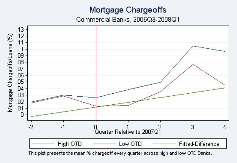
The Review of Financial Studies / v 24 n 6 2011

  in raising external capital might prohibit a bank from lending up to the first-best
  level (Stein 1998). Financial innovations naturally arise as a market response to
  these frictions (Tufano 2003; Allen and Gale 1994). The originate-to-distribute
  (OTD) model of lending, where the originator of loans sells them to third par-
  ties, emerged as a solution to some of these frictions. This model allows the
  originating financial institution to achieve better risk-sharing with the rest of
  the economy,1 economize on regulatory capital, and achieve better liquidity
  risk management.2
     These benefits of the OTD model come at a cost. As the lending practice
  shifts from an originate-to-hold to an originate-to-distribute model, it begins
  to interfere with the originating banks’ screening and monitoring incentives
  (Pennacchi 1988; Gorton and Pennacchi 1995; Petersen and Rajan 1994;
  Parlour and Plantin 2008). It is this cost of the OTD model that lies at the
  root of our analysis. Banks make lending decisions based on a number of bor-
  rower characteristics. While some of these characteristics are easy to credibly
  communicate to third parties, there are soft pieces of information that cannot
  be easily verified by parties other than the originating institution itself. Thus,

                                                                                                                         Downloaded from rfs.oxfordjournals.org at :: on September 14, 2011
  as the originating institution sheds the credit risk, and as the distance between
  the originator and the ultimate holder of risk increases, loan officers’ ex ante
  incentives to collect soft information decrease (see Stein 2002 and Rajan, Seru,
  and Vig 2009). If the ultimate holders of credit risk do not completely appre-
  ciate the true credit risk of mortgage loans, then it is easy to see the resulting
  dilution in the originator’s screening incentives. However, it is not a neces-
  sary condition for the dilution in screening standards to occur. For example, if
  the cost of communicating soft information is so high that all originators are
  pooled together by the outside investors, then the originator’s ex ante screening
  incentive goes down even without pricing mistakes by the ultimate investors.
  The screening incentives can deteriorate further if credit-rating agencies make
  mistakes, as some observers have argued, in assessing the true credit risk of
  mortgage-backed securities.
     Our key hypothesis is that banks with aggressive involvement in the OTD
  market had lower screening incentives, which in turn resulted in the origi-
  nation of loans with excessively poor soft information by these banks. The
  OTD model of lending allowed them to benefit from the origination fees with-
  out bearing the credit risk of the borrowers. As long as the secondary market
  for mortgage sale was functioning normally, they were able to easily offload
  these loans to third parties.3 When the secondary mortgage market came under

1 Allen and Carletti (2006) analyze conditions under which credit-risk transfer from banking to some other sector
  leads to risk-sharing benefits. They also argue that under certain conditions, these risk-transfer tools can lead to
  welfare-decreasing outcomes.
2 See Drucker and Puri (2005) for a survey of different theories behind loan sales.

3 The mortgage market was functioning normally until the first quarter of 2007. In March 2007, several subprime
  mortgage lenders filed for bankruptcy, providing some early signals of the oncoming mortgage crisis. The sign of
  stress in this market became visibly clear by the middle of 2007 (Greenlaw, Hatzius, Kashyap, and Shin 2008).

  1882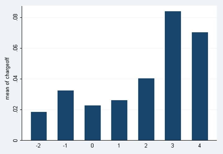
Originate-to-distribute Model and the Subprime Mortgage Crisis

pressure in the middle of 2007, banks with a higher volume of OTD loans were
stuck with large quantities of relatively inferior-quality mortgage loans. It can
take about two to three quarters from the origination to the sale of these loans in
the secondary market (Gordon and D’Silva 2008). In addition, the originators
typically guarantee the loan performance for the first 90 days of loans (Mishkin
2008). If banks with a high volume of OTD loans in the pre-disruption pe-
riod were originating loans of inferior quality, then in the immediate post-
disruption period, such banks are likely to be left with a disproportionately
large quantity of poor loans. We use the sudden drop in liquidity in the sec-
ondary mortgage market to identify the effect of OTD lending on mortgage
quality.
   We define the period up to the first quarter of 2007 as the pre-disruption
period, and later quarters as post-disruption. We first confirm that banks with
a large quantity of origination in the immediate pre-disruption period were
unable to sell their OTD loans in the post-disruption period. We then show
that banks with higher participation with the OTD model in the pre-disruption
period had significantly higher mortgage chargeoffs and defaults by their

                                                                                      Downloaded from rfs.oxfordjournals.org at :: on September 14, 2011
borrowers in the immediate post-disruption period. In addition, the mortgage
chargeoffs and borrower defaults are higher for those banks that were unable
to sell their pre-disruption OTD loans; i.e., for banks that were left with large
quantities of undesired mortgage portfolios.
   Overall, these results suggest that OTD loans were of inferior quality, and
banks that were stuck with these loans in the post-disruption period had dis-
proportionately higher chargeoffs and borrower defaults. In order to provide
convincing support for the diluted screening incentives hypothesis, it is im-
portant to rule out the effect of observable differences in the quality of loans
issued by high- and low-OTD banks on mortgage default rate. We conduct sev-
eral tests using detailed loan-level data from the Home Mortgage Disclosure
Act (HMDA) to address this issue. In these tests, we compare the default rate
of high- and low-OTD banks that are matched along several dimensions of
borrowers’ observable default risk, properties’ location, and the bank’s char-
acteristics. We show that our results remain strong in the matched subsamples.
Thus, the effect of OTD lending on mortgage default rates is not an artifact of
observable differences in the borrowers’ credit risk, the geographical location
of high- and low-OTD banks, or differences in the originating bank’s other
characteristics, such as size and cost of capital.
   We continue our investigation by analyzing the interest rates charged by
high- and low-OTD banks during the pre-disruption period. If a bank screens
its borrowers carefully on unobservable dimensions, then it is more likely to
charge different interest rates to observationally similar borrowers (see Rajan,
Seru, and Vig 2009). Therefore, we expect to find a wider distribution of inter-
est rates for the same set of observable characteristics for a bank that screens
its borrowers more actively. Based on this idea, we compare the distribution of
interest rates charged by the high- and low-OTD banks. Consistent with the lax

                                                                             1883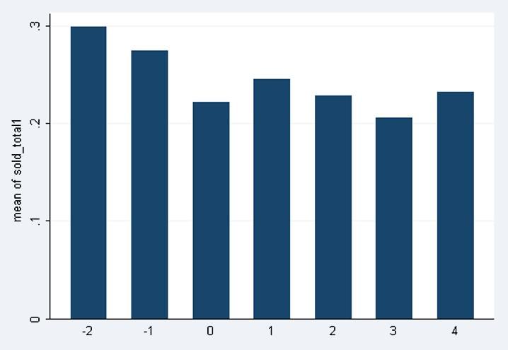
The Review of Financial Studies / v 24 n 6 2011

  screening hypothesis, we find evidence of tighter distribution for the high-OTD
  banks in our sample.
     In our final test, we focus on the determinants of poor screening by the high-
  OTD banks. We find that the effect of pre-disruption OTD lending on mortgage
  default rates is stronger among banks with lower regulatory capital. If banks
  used the OTD model of lending in response to binding capital constraints, then
  banks with a lower capital base should do no worse than the well-capitalized
  banks. In contrast, theoretical models such as Thakor (1996) and Holmstrom
  and Tirole (1997) suggest that banks with lower capital have a lower screening
  incentive due to the risk-shifting problem. Our results support the presence
  of lax screening incentives behind the origination of such loans. We also find
  that the effect of OTD loans on mortgage default is concentrated among banks
  with a lower dependence on demand deposits.4 The result supports the view
  that demand deposits worked as a governance device for commercial banks,
  as argued by Calomoris and Kahn (1991), Flannery (1994), and Diamond and
  Rajan (2001). Our study shows that banks that were primarily funded by non-
  demandable or market-based wholesale debt were the main originators of poor-

                                                                                                                     Downloaded from rfs.oxfordjournals.org at :: on September 14, 2011
  quality OTD loans.
     There is a growing literature in this area, with important contributions from
  Keys et al. 2010; Mian and Sufi 2010; Loutskina and Strahan 2008; Doms,
  Furlong, and Krainer 2007; Mayer and Pence 2008; Dell’Ariccia, Igan, and
  Laeven 2008; Demyanyk and Van Hemert 2009; and Titman and Tsyplakov
  2010. We make three unique contributions to the literature. This is one of
  the first academic studies that compares default rates of banks that originated
  loans to sell to third parties with banks that originated loans for their own
  portfolios. Our findings complement those of Keys et al. (2010), who ana-
  lyze default rates of securitized loans above and below the FICO score of
  620. In addition to the advantage of comparing sold versus retained loans,
  our analysis also shows that the dilution in screening standards was not con-
  fined to a particular range of borrowers’ FICO scores. Instead, it was a far
  more widespread phenomenon that occurred throughout the banking sector.
  Second, we focus on lending decisions of institutions that are directly originat-
  ing loans from borrowers or through their brokers. Thus, our study analyzes
  the screening behavior of economic agents that are directly responsible for
  originating loans at the front end of the lending-securitization channel. Third,
  our study advances the literature by showing that a bank’s capital position
  and reliance on non-demandable debt have significant effects on its screening
  incentives.
     Overall, our findings have important implications for banking regulations. In
  addition, we contribute to the credit-risk pricing literature by showing that in
  an information-sensitive asset market, the issuer’s capital position and liability

4 Since the capital structure and the demand deposit mix of large banks are generally very different from those of
  the small banks, we pay careful attention to the effect of bank size in these tests.

  1884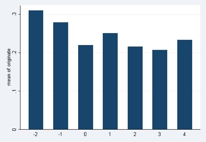
Originate-to-distribute Model and the Subprime Mortgage Crisis

   structure have important implications for the pricing of assets in the secondary
   market. It is important to note that our results come from a period of turmoil
   in the financial markets. To draw strong policy implications, one obviously
   has to compare these costs of securitization with the potential benefits of risk-
   management tools (Stulz 1984; Smith and Stulz 1985; Froot, Scharfstein, and
   Stein 1993; Froot and Stein 1998; Drucker and Puri 2009).5 It is also worth
   pointing out that the role of other macroeconomic factors, such as the aggregate
   borrowing and savings rate and monetary policies across the globe, cannot be
   ignored as a potential explanation for the crisis (see Allen 2009). Our study is
   essentially cross-sectional in nature, which limits our ability to comment on
   the role of these macroeconomic factors.
      The rest of the article is organized as follows. Section 1 describes the data
   and provides descriptive statistics. Section 2 presents empirical results relat-
   ing OTD market participation to mortgage defaults. Section 3 provides the
   matched sample results. Section 4 explores the linkages with capital position
   and liability structure, and Section 5 concludes.

                                                                                                                      Downloaded from rfs.oxfordjournals.org at :: on September 14, 2011
1. Data
   We use two sources of data for our study: the call report database for bank in-
   formation and the HMDA (Home Mortgage Disclosure Act) database for loan
   details. All Federal Deposit Insurance Corporation (FDIC)-insured commer-
   cial banks are required to file call reports with the regulators on a quarterly
   basis. These reports contain detailed information on the bank’s income state-
   ment, balance-sheet items, and off-balance-sheet activities. The items required
   to be filed in this report change over time to reflect the changing nature of bank-
   ing business. As the mortgage sale and securitization activities grew in recent
   years, there have been concomitant improvements in the quality of reporting
   with respect to these items as well.
      Beginning with the third quarter of 2006, banks started to report two key
   items regarding their mortgage activities: (a) the origination of 1–4 family
   residential mortgages during the quarter with a purpose to resell in the market;
   and (b) the extent of 1–4 family residential mortgages actually sold during the
   quarter. These variables allow us to measure the extent of participation in the
   OTD market as well as the extent of loans that were actually offloaded by a
   bank in a given quarter. Both items are provided in schedule RC-P of the call
   report. This schedule is required to be filed by banks with $1 billion or more in
   total assets and by smaller banks if they exceed $10 million in their mortgage-
   selling activities. The data, in effect, are available for all banks that participate
   significantly in the OTD market.

 5 See also Ashcraft and Santos (2008) for a study on the costs and benefits of credit default swaps, and Gande and
   Saunders (2007) for the effect of the secondary loan sales market on the bank-specialness.

                                                                                                           1885
The Review of Financial Studies / v 24 n 6 2011
We construct our key measure of OTD activity as the ratio of loans origi-
nated for resale during the quarter scaled by the beginning of the quarter mort-
gage loans of the bank. This ratio captures the extent of a bank’s participation
in the OTD market as a fraction of its overall mortgage portfolio. We measure
the extent of selling in the OTD market as the ratio of loans sold during the
quarter scaled by the mortgage loans from the beginning of the quarter.
We obtain two measures of mortgage quality from the call reports: (1)
chargeoffs on 1–4 family residential mortgages; and (2) non-performing assets
(NPAs) for this category; i.e., mortgage loans that are past due or delinquent.
We use net chargeoffs (net of recoveries) as the first proxy of loan quality. It
measures the immediate effect of mortgage defaults on a bank’s profitability.
However, chargeoffs may be subject to the reporting bank’s discretionary ac-
counting rules. Mortgage NPAs, on the other hand, are free from this bias and
provide a more direct measure of the borrowers’ default rate.
We get information on the banks’ assets, profitability, mortgage loans, liq-
uidity ratio, capital ratios, and several other variables from the call report. It
is important to construct these variables in a consistent manner across quar-
Downloaded from rfs.oxfordjournals.org at :: on September 14, 2011
ters since the call report’s reporting format changes somewhat over time. Our
study spans only seven quarters—from 2006Q3, the first quarter with OTD
data available, to 2008Q1. The reporting requirement has been fairly stable
over this time period, and we check every quarter’s format to ensure that our
data are consistent over time. We provide detailed information on the variables
and construction of key ratios in the Appendix.
We obtain detailed loan-level information from the HMDA database. The
HMDA was enacted by Congress in 1975 to improve reporting requirements
in the mortgage lending business. The HMDA database is an annual database
that contains loan-by-loan information on borrower quality, applicant’s de-
mographic information, and interest rate on the loan if it exceeds a certain
threshold. We match the call report and HMDA database for 2006 to obtain in-
formation on the quality of borrowers and geographical location of loans made
by banks during the pre-disruption period.
1.1 Descriptive statistics
Our sample consists of all banks with available data on mortgage origination
for resale from 2006Q3 to 2008Q1. We intersect this sample with banks cov-
ered in the HMDA database in 2006. We create a balanced panel of banks,
requiring the sample bank to be present in all seven quarters. This filter re-
moves only a few banks and does not change any of our results. We impose
this filter because we want to exploit the variation in mortgage default rates of
the same bank over time as the mortgage market passed through the period of
stress.
We begin the discussion of descriptive statistics with a few charts. In
Figure 1, we plot the quarterly average of loans originated for resale as a
1886Originate-to-distribute Model and the Subprime Mortgage Crisis
Figure 1
Mortgage originated for distribution over time
Downloaded from rfs.oxfordjournals.org at :: on September 14, 2011
The figure plots the ratio of OTD loans to total mortgages on a quarterly basis. We plot the average value of this
ratio across all banks with available information in the sample. Quarter zero corresponds to the quarter ending
on March 31, 2007.
fraction of the bank’s outstanding mortgage loans (measured at the beginning
of the quarter). This ratio measures the bank’s desired level of credit-risk trans-
fer through the OTD model. The ratio averaged just below 30% during 2006Q3
and 2006Q4 and dropped to about 20% in the subsequent quarters. The drop
is consistent with the popular belief that the OTD market came under tremen-
dous stress during this period. Figure 2 plots the quarterly average of loans sold
scaled by the beginning of the quarter loans outstanding. This measures the ex-
tent of credit-risk transfer that the bank was actually able to achieve during the
quarter. There is a noticeable decline in the extent of loan sales starting with
2007Q1. As we show later, the decline was especially pronounced in banks that
were aggressively participating in the OTD market in or before 2007Q1. Over-
all, these graphs show that the extent of loan origination and loans transferred
to other parties came down appreciably over this time period.
Figure 3 plots the average percentage chargeoff on 1–4 family residential
mortgage loans on a quarterly basis. As expected, the quarterly chargeoffs
have increased steadily since 2007Q1. The chargeoffs increased fourfold from
2007Q1 to 2007Q4—a very significant increase for highly leveraged finan-
cial institutions. We find a similar trend for non-performing mortgages as well
(unreported).
Table 1 provides the descriptive statistics of other key variables used in the
study. We winsorize data at 1% from both tails to minimize the effects of out-
liers. The average bank in our sample has an asset base of $5.9 billion (median
$1.1 billion). These numbers show that our sample represents relatively large
1887The Review of Financial Studies / v 24 n 6 2011
Figure 2
Mortgage sold over time
Downloaded from rfs.oxfordjournals.org at :: on September 14, 2011
The figure plots the extent of loans sold as a fraction of mortgages outstanding as of the beginning of the quarter.
We plot the average value of this ratio across all banks with available information in the sample. Quarter zero
corresponds to the quarter ending on March 31, 2007.
Figure 3
Mortgage chargeoff over time
The figure plots the average net chargeoff as a percentage of mortgage outstanding on a quarterly basis. Quarter
zero corresponds to the quarter ending on March 31, 2007.
banks, due to the fact that we require data on OTD mortgage origination and
sale for a bank to be available to be included in our sample. We provide the
distribution of other key variables in the table. These numbers are in line with
other studies involving large bank samples.
1888Originate-to-distribute Model and the Subprime Mortgage Crisis
Table 1
Summary statistics
variable N mean p50 min max
ta 5397.00 5.92 1.05 0.06 168.65
mortgage/ta 5397.00 0.17 0.15 0.01 0.49
cil/ta 5397.00 0.11 0.10 0.00 0.39
td/ta 5397.00 0.78 0.80 0.44 0.92
dd/td 5397.00 0.09 0.08 0.01 0.33
leverage 6636.00 0.90 0.91 0.77 0.94
nii/ta 5397.00 0.89 0.87 0.32 1.51
chargeoff(%) 5397.00 0.04 0.00 −0.07 0.79
npa/ta(%) 5397.00 0.73 0.44 0.00 5.40
mortnpa(%) 5397.00 2.03 1.35 0.00 13.86
tier1cap 5397.00 0.11 0.10 0.07 0.29
liquid 5397.00 0.15 0.12 0.02 0.50
absgap 5397.00 0.14 0.11 0.00 0.51
preotd 771.00 0.23 0.05 0.00 3.06
This table provides the summary statistics of key variables used in the study. All variables are computed using
call report data for seven quarters starting from 2006Q3 and ending in 2008Q1. We provide the number of
observations (N), mean, median, minimum, and maximum values for each variable. ta is total assets in billions
of dollars; mortgage/ta is the ratio of 1–4 family residential mortgages outstanding to total assets; cil/ta is the
ratio of commercial and industrial loans to total assets; td/ta is the ratio of total deposits to total assets; dd/td is
the ratio of demand deposits to total deposits; nii/ta is the ratio of net interest income to total assets; chargeoff
Downloaded from rfs.oxfordjournals.org at :: on September 14, 2011
measures the chargeoff on mortgage portfolio (net of recoveries) as a percentage of mortgage assets; npa/ta
is the ratio of non-performing assets to total assets; mortnpa is the ratio of non-performing mortgages to total
mortgages; tier1cap measures the ratio of tier-one capital to risk-adjusted assets; liquid is the bank’s liquid assets
to total assets ratio, absgap is the absolute value of one-year maturity gap as a fraction of total assets. preotd
measures the originate-to-distribute loans, i.e., mortgages originated with a purpose to sell, as a fraction of total
mortgages. This variable is constructed at the bank level based on its average quarterly values during 2006Q3,
2006Q4, and 2007Q1.
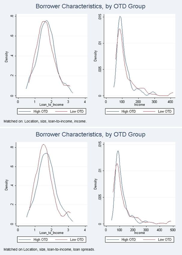
Figure 4 provides a graphical preview of our results. We take the average
value of OTD ratio for every bank during 2006Q3, 2006Q4, and 2007Q1;
i.e., during quarters prior to the serious disruption in the market. We call this
variable preotd.6 We classify banks into high- or low-OTD groups based on
whether they fall into the top or bottom one-third of the preotd distribution. We
track mortgage chargeoffs of these two groups of banks over quarters and plot
them in Figure 4. Consistent with our earlier graph on the aggregate charge-
offs, this figure shows that both groups have experienced a significant increase
in chargeoffs over time. However, there is a remarkable difference in their
slopes. While both groups started at similar levels of chargeoffs in 2006Q3
and they show parallel trends before the beginning of the crisis, the high-OTD
group’s chargeoffs increased five times by the end of the sample period as
compared with a significantly lower increase of about two to three times for
the low-OTD group. We also plot the fitted difference between the two groups
over time. The fitted difference measures the difference in the rate of increase
in chargeoffs across the two groups and therefore gives a graphical snapshot
of the difference-in-difference estimation results. The fitted difference shows a
6 Our results are robust to alternative ways of constructing this variable; for example, by averaging over only
2006Q3 and 2006Q4 or by only taking 2007Q1 value as the measure of preotd.
1889The Review of Financial Studies / v 24 n 6 2011
Downloaded from rfs.oxfordjournals.org at :: on September 14, 2011
Figure 4
Mortgage chargeoff and OTD participation
The figure plots the average net chargeoff (as a percentage of mortgage outstanding) on the bank’s mortgage
portfolio across two groups of banks sorted on the basis of their participation in the OTD market prior to March
31, 2007.
remarkable linear increase over this time period. The difference in default rate
becomes especially high after a couple of quarters from the onset of the crisis.
In summary, we find that banks with higher OTD participation before the
subprime mortgage crisis increased their chargeoffs significantly more than
banks with lower OTD. Are these differences significant after accounting for
differences in bank characteristics and the quality of borrowers they face? And
why does this difference exist across the two groups? We explore these ques-
tions through formal econometric tests in the rest of the article.
2. Mortgage Default Rate and OTD
We first establish that there was a significant drop in the extent of mortgages
sold in the secondary market in the post-disruption period. We follow this up
with our main test that examines the relationship between a bank’s mortgage
default rate and the extent of its participation in the OTD market.
2.1 Empirical design and identification strategy
Our key argument is that banks with aggressive involvement in the OTD model
of lending did not actively screen their borrowers along the soft informa-
tion dimension. The OTD model allowed them to benefit from the origination
fees without bearing the ultimate credit risk of the borrowers. These banks
originated large amounts of loans with inferior soft information, which were
subsequently sold to investors. As long as the secondary loan market had
1890Originate-to-distribute Model and the Subprime Mortgage Crisis
enough liquidity, banks were able to offload their originated loans without
any disruption. The delay from origination to the final sale of these loans did
not impose significant credit risk on the originating banks during normal pe-
riods. However, when the secondary mortgage market came under pressure
in the middle of 2007, banks with high-OTD loans were stuck with dispro-
portionately large amounts of inferior-quality mortgage loans. The problem
was exacerbated by the early pay default warranties that the sellers of OTD
loans typically provide to their buyers for the first 90 days after the loan sale
(Mishkin 2008). Therefore, immediately after the liquidity shock of summer
2007, these banks were left with disproportionately large amounts of OTD
mortgage loans that they had originated with an intention to sell but could not
sell. If these loans had relatively lower screening standards, then we expect
to find relatively higher mortgage default rates for high-OTD banks in quar-
ters immediately following the onset of the crisis as compared with otherwise
similar low-OTD banks that originated most of their loans with an intention to
keep them on their balance sheets.
To test this hypothesis in an idealized experimental setting, we need two ran-
Downloaded from rfs.oxfordjournals.org at :: on September 14, 2011
domly selected groups of banks that are identical in every respect except for
their involvement in the OTD method of lending. To be more precise, we want
to compare banks with varying intensity of OTD lending that have made loans
to borrowers with observationally similar risk characteristics. This will allow
us to estimate the effect of OTD lending on the screening efforts of banks along
the soft information dimension without contaminating the results from differ-
ences in observable risk characteristics of the borrowers. Because we have
only observational data, we control for these differences by including several
bank and borrower characteristics in the regression model. More importantly,
we conduct our tests in a difference-in-difference setting with carefully cho-
sen matched samples of high- and low-OTD banks. In these tests, we attempt
to find pairs of banks that are similar and have made loans to observationally
similar borrowers before the crisis. Then we exploit differences along the OTD
dimension in these samples to estimate the effect of OTD lending on screening
efforts.
2.1.1 Extent of mortgage resale. Since our identification strategy relies on
banks’ inability to sell their loans in the secondary markets, we first document
evidence in support of this argument. We estimate the following model:
k=K
X
soldit = β0 + β1 aftert + β2 preotdi + β3 aftert ∗ preotdi + β X it + it .
k=1
soldit measures bank i’s mortgage sale as a fraction of its total mortgage loans
at the beginning of quarter t.7 As described earlier, preotdi is a time-invariant
7 Our results are similar if we add the mortgages originated during the quarter in the denominator.
1891The Review of Financial Studies / v 24 n 6 2011
variable that measures the extent of bank i’s participation in the OTD market
prior to the disruption in this market in the middle of 2007. We expect to find
a positive and significant coefficient on this variable because banks with large
OTD loans, almost by construction, are more likely to sell large quantities
of these loans in the secondary market. a f tert is an indicator variable that
equals one for quarters after 2007Q1, and zero otherwise. The coefficient on
this variable captures the difference in mortgages sold before and after the
crisis. The coefficient on the interaction term pr eotdi ∗ a f tert is the estimate
of interest. This coefficient measures the change in the intensity of loans sold
around the disruption period across banks with different degrees of pr eotd.
We control for several bank characteristics denoted by vector X it to account
for the effect of bank size, liquidity, maturity gap, and the ratio of commercial
and industrial loans to total assets. More importantly, we also include a variable
pr emor tgage that measures the extent of mortgages made by the bank during
the pre-disruption period. This variable is computed as the average of the ratio
of mortgage loans to total assets during 2006Q3, 2006Q4, and 2007Q1. We
include this variable and its interaction with a f ter to separate the effect of
Downloaded from rfs.oxfordjournals.org at :: on September 14, 2011
high-mortgage banks from the high-OTD banks.8
To provide a benchmark specification, we first estimate this model using the
OLS method. All standard errors are clustered at the bank level to account for
correlated errors across all quarters for the same bank (see Bertrand, Duflo,
and Mullainathan 2004). In the OLS model, we include indicator variables for
the bank’s state to control for state-specific differences in mortgage activities.
Results are provided in Model 1 of Table 2. As expected, we find a large and
positive coefficient on the pr eotd variable. The coefficient on the interaction
of a f ter and pr eotd is negative and highly significant. In this specification,
we find a positive coefficient on the a f ter dummy variable. In unreported tests,
we estimate an OLS regression of soldit on a f ter and obtain a coefficient of
−0.031(t − stat = −1.97) on a f ter . Therefore, the sharp decline in the loan
resale is concentrated within the set of high pr eotd banks.
We provide bank fixed-effect estimation results in Models 2 and 3 of Table 2.
This estimation method is more appealing, as it controls for bank-specific un-
observable effects and allows us to more precisely estimate the effect of disrup-
tion in the mortgage market on the high-OTD banks. pr eotd and pr emor tgage
are omitted from this model because they are captured in the bank fixed ef-
fects. Our identification comes from the interaction of a f ter with pr eotd.
In Model 2, we find a significant negative coefficient on the interaction term,
which confirms that banks with large OTD loans in the pre-disruption period
suffered a significant decline in mortgage resale during the post-disruption pe-
riod. In unreported tests, we estimate this model without the interaction term
a f ter ∗ pr eotd and find a significant negative coefficient on a f ter (coefficient
8 Our results are similar without the inclusion of the pr emor tgage variable in the regression models.
1892Originate-to-distribute Model and the Subprime Mortgage Crisis
Table 2
Intensity of mortgages sold
Model 1 Model 2 Model 3
Estimate t-stat Estimate t-stat Estimate t-stat
preotd 0.9591 (54.64)
premortgage 0.0403 (0.85)
after 0.0273 (1.95) 0.0182 (1.23) 0.0205 (1.24)
after*preotd −0.1889 (−3.34) −0.2037 (−3.74) −0.2120 (−3.86)
after*premortgage 0.0163 (0.21) 0.0235 (0.29) 0.0428 (0.49)
logta −0.0031 (−0.54) 0.1475 (2.88) 0.1575 (2.44)
cil/ta −0.0248 (−0.22) −0.8606 (−2.74) −0.7744 (−2.40)
liquid 0.0339 (0.48) −0.0292 (−0.21) 0.0570 (0.38)
absgap −0.0320 (−0.55) 0.2866 (2.79) 0.3171 (2.82)
R2 0.8156 0.9039 0.9054
N 4476 4476 4100
State dummies Yes No No
Bank fixed effect No Yes Yes
Exclude large banks No No Yes
This table provides the regression results of the following model:
k=K
X
soldit = β0 + β1 a f tert + β2 pr eotdi + β3 a f tert ∗ pr eotdi + β X + it .
Downloaded from rfs.oxfordjournals.org at :: on September 14, 2011
k=1
The dependent variable, soldit , measures bank i ’s mortgage sale as a fraction of its total mortgage loans at the
beginning of quarter t . a f tert is a dummy variable that is set to zero for quarters before and including 2007Q1,
and one after that. pr eotdi is the average value of OTD mortgages to total mortgages during quarters 2006Q3,
2006Q4, and 2007Q1. X stands for a set of control variables. Model 1 is estimated using the OLS method.
Models 2 and 3 are estimated with bank fixed effects. Model 3 excludes banks with more than $10 billion in
assets. These models omit pr eotd and pr emor tgage as right-hand-side variables since they remain constant
across all seven quarters for a given bank. premortgage is the average ratio of mortgage assets to total assets
for 2006Q3, 2006Q4, and 2007Q1. logta measures the log of total assets; cil/ta is the ratio of commercial and
industrial loans to total assets; liquid is the bank’s liquid assets to total asset ratio; absgap is the absolute value of
one-year maturity gap as a fraction of total assets. Adjusted R-squared and number of observations are provided
in the bottom rows. All standard errors are clustered at the bank level.
estimate of −0.0251 with t-statistics of −2.74). These findings show that the
decline in mortgage resale is concentrated among high pr eotd banks. In Model
3, we re-estimate the fixed-effect model after removing banks with more than
$10 billion in asset size from the sample because it is often argued that large
money-centric banks have a different business model than regional and local
banks. We find that our results are equally strong after excluding these large
banks from the sample.
These results are economically significant as well. For example, a one-
standard-deviation increase in OTD lending prior to the disruption results in
a decline of 10% in selling intensity after the crisis based on the estimates of
Model 2. Overall, these results are consistent with our assertion that the dis-
ruption in the mortgage market created warehousing risk for the banks, which
in turn led to an accumulation of undesired loans; i.e., loans that were initially
intended to be sold but could not be sold due to an unexpected decline in the
market conditions.
1893The Review of Financial Studies / v 24 n 6 2011
2.2 Mortgage defaults
We now estimate the effect of OTD lending on a bank’s quarterly mortgage
default rates with the following bank fixed-effect regression model:
defaultit = μi + β1 aftert + β2 aftert ∗ preotdi + β3 aftert ∗ premortgagei
k=K
X
+ β X it + it .
k=1
The dependent variable of this model measures the default rate of the mortgage
portfolio of bank i in quarter t. We use two measures of default: net-chargeoffs
and non-performing mortgages; i.e., mortgages that are in default for more than
30 days. We scale them by the bank’s total mortgage loans measured as of the
beginning of the quarter. μi stands for bank fixed effects, and X it is a vec-
tor of bank characteristics.9 The coefficient on the a f ter variable captures the
time trend in default rate before and after the mortgage crisis. The coefficient
on the interaction term (i.e., a f tert ∗ pr eotdi ) measures the change in char-
geoffs/NPAs around the crisis period across banks with varying intensities of
Downloaded from rfs.oxfordjournals.org at :: on September 14, 2011
participation in the OTD market prior to the crisis. Said differently, β2 mea-
sures the change in default rate for banks that originated loans primarily to sell
them to third parties, as compared with the corresponding change for banks
that originated loans primarily to retain them on their own balance sheets. We
include the interaction of a f ter with pr emor tgage to ensure that the relation-
ship between OTD loans and mortgage performance is not simply an artifact
of higher involvement in mortgage lending by higher OTD banks.10
We control for a host of bank characteristics that can potentially affect the
quality of mortgage loans. We control for the bank’s size by including the log
of total assets in the regression model. We include the ratio of commercial and
industrial loans to total assets to control for the broad business mix of the bank.
A measure of the 12-month maturity gap is included to control for the interest-
rate risk faced by the banks. Finally, we include the ratio of liquid assets to
total assets to control for the liquidity position. The last three variables broadly
capture the extent and nature of credit risk, interest-rate risk, and liquidity risk
faced by the banks.
Table 3 provides the results. We provide results for the entire sample in
Models 1 and 2. In Models 3 and 4, we exclude large banks with asset size
more than $10 billion from the sample. We find that the extent of participation
in the OTD market during the pre-disruption period has a significant effect
9 In an alternative specification, we also estimate this model without bank fixed effects (similar to the one de-
scribed in the previous section for the extent of mortgage resale). The advantage of this model is that it also
allows us to estimate the coefficient on pr eotd . However, we prefer the bank fixed-effect approach as it allows
us to control for unobservable factors that are time-invariant and unique to a bank. All key results remain similar
for the alternative econometric model.
10 We re-estimate these models without including the interaction of a f ter and pr emor tgage and obtain similar
results.
1894Originate-to-distribute Model and the Subprime Mortgage Crisis
Table 3
Mortgage defaults
All Banks Excludes Large Banks
Model 1 Model 2 Model 3 Model 4
Chargeoffs NPA Chargeoffs NPA
Dependent Var: Estimate t-stat Estimate t-stat Estimate t-stat Estimate t-stat
after 0.0116 (1.91) 0.3411 (3.03) 0.0134 (2.03) 0.3076 (2.52)
after*preotd 0.0420 (2.76) 0.4439 (2.44) 0.0428 (2.76) 0.4015 (2.21)
after*premortgage 0.0060 (0.21) 0.6600 (1.22) −0.0062 (−0.20) 0.4261 (0.82)
logta 0.0925 (4.15) 0.2266 (0.51) 0.0776 (2.67) 0.6896 (1.42)
cil/ta 0.2010 (1.65) 2.6103 (1.37) 0.1662 (1.32) 2.2626 (1.13)
liquid 0.0745 (1.24) 1.3732 (0.90) 0.1089 (1.64) −0.1540 (−0.14)
absgap −0.0672 (−1.59) −3.2639 (−3.85) −0.0742 (−1.64) −3.1248 (−3.66)
R2 0.3805 0.7297 0.3621 0.7135
N 5397 5397 4977 4977
This table provides the regression results of the following fixed-effects model:
k=K
X
defaultit = μi + β1 aftert + β2 aftert ∗ preotdi + β X + it .
k=1
The dependent variable, de f aultit , is measured by either the mortgage chargeoffs or the non-performing mort-
Downloaded from rfs.oxfordjournals.org at :: on September 14, 2011
gages (scaled by the outstanding mortgage loans) of bank i during quarter t . a f tert is a dummy variable that is
set to zero for quarters before and including 2007Q1, and one after that. pr eotdi is the average value of OTD
mortgages to total mortgages during quarters 2006Q3, 2006Q4, and 2007Q1. μi denotes bank fixed effects;
X stands for a set of control variables. premortgage is the average ratio of mortgage assets to total assets for
2006Q3, 2006Q4, and 2007Q1. logta measures the log of total assets; cil/ta is the ratio of commercial and in-
dustrial loans to total assets; liquid is the bank’s liquid assets to total assets ratio; absgap is the absolute value of
one-year maturity gap as a fraction of total assets. Adjusted R-squared and number of observations are provided
in the bottom rows. All standard errors are clustered at the bank level.
on a bank’s mortgage default rates during the post-disruption quarters. In the
chargeoff regression model (Model 1), we find a positive and significant co-
efficient of 0.0420 on a f ter ∗ pr eotd. In Model 2, we repeat the analysis
with non-performing mortgages as the measure of loan quality and again find
a positive and significant coefficient on the interaction term. These effects are
economically large as well. For example, based on the estimates of Model 2, a
one-standard-deviation increase in pr eotd results in an increase of about 11%
in the mortgage default rate as compared with the unconditional sample mean.
We repeat our analysis after excluding large banks from the sample and obtain
similar results.11
In our next test, we model mortgage defaults as a function of the extent
of OTD loans that a bank is stuck with. For every bank in the sample, we
create a measure of stuck loans in the following manner. We first compute
the quarterly average of OTD loans originated during the pre-crisis quarters;
i.e., during the quarters 2006Q3, 2006Q4, and 2007Q1. From this, we subtract
the quarterly average of loans sold during the post-crisis periods; i.e., during
11 In an unreported robustness exercise, we drop the first two quarters after the beginning of the crisis from our
sample. We do so to allow more time for the mortgages to default after the beginning of the crisis. Our results
become slightly stronger for this specification.
1895The Review of Financial Studies / v 24 n 6 2011
Table 4
Mortgage default and inability to sell
All Banks Excludes Large Banks
Model 1 Model 2 Model 3 Model 4
Chargeoffs NPA Chargeoffs NPA
Dependent Var: Estimate t-stat Estimate t-stat Estimate t-stat Estimate t-stat
after 0.0131 (2.18) 0.3113 (2.81) 0.0148 (2.25) 0.2791 (2.35)
after*stuck 0.0922 (3.03) 1.4342 (3.64) 0.0940 (3.02) 1.2756 (3.39)
after*premortgage 0.0000 (0.00) 0.5888 (1.11) −0.0110 (−0.35) 0.3892 (0.75)
logta 0.1004 (4.64) 0.3684 (0.85) 0.0855 (3.02) 0.8078 (1.67)
cil/ta 0.1964 (1.62) 2.3276 (1.25) 0.1675 (1.34) 2.0930 (1.07)
liquid 0.0633 (1.05) 1.1788 (0.83) 0.1047 (1.60) −0.2045 (−0.19)
absgap −0.0603 (−1.43) −3.1394 (−3.79) −0.0690 (−1.54) −3.0421 (−3.59)
R2 0.3818 0.7330 0.3635 0.7162
N 5397 5397 4977 4977
This table provides regression results for the following fixed-effect model:
k=K
X
de f aultit = μi + β1 a f tert + β2 a f tert ∗ stucki + β X + it .
k=1
The dependent variable, de f aultit , is measured by either the mortgage chargeoffs or the non-performing mort-
Downloaded from rfs.oxfordjournals.org at :: on September 14, 2011
gages of bank i during quarter t . a f tert is a dummy variable that is set to zero for quarters before and including
2007Q1, and one after that. stucki measures the difference between loans originated before 2007Q1 and loans
sold after this quarter. μi denotes bank fixed effects; X stands for a set of control variables. premortgage is the
average ratio of mortgage assets to total assets for 2006Q3, 2006Q4, and 2007Q1. logta measures the log of
total assets; cil/ta is the ratio of commercial and industrial loans to total assets; liquid is the bank’s liquid assets
to total assets ratio; absgap is the absolute value of one-year maturity gap as a fraction of total assets. Adjusted
R-squared and number of observations are provided in the bottom rows. All standard errors are clustered at the
bank level.
2007Q2 to 2008Q1. We scale the difference by the bank’s average mortgage
assets during the pre-crisis quarters. This variable refines the earlier pr eotd
measure by subtracting the extent of loans that a bank could actually sell in
the post-disruption period. This variable allows us to more directly analyze
the effect of loans that a bank had originated to distribute but was unable to
distribute due to the drop in liquidity in the secondary market.12
We re-estimate the de f ault regression model by replacing pr eotd with
stuck. Results are presented in Table 4. We find a large positive coefficient
on the interaction term pr eotd ∗ stuck in Model 1. In unreported tests, we run
a horse race between a f ter ∗ pr eotd and a f ter ∗ stuck and find that the effect
of OTD loans on mortgage chargeoffs mainly comes from the variation in the
stuck variable. Similar results hold for mortgage default rate using NPA as the
dependent variable (see Model 2). Models 3 and 4 show that our results are
robust to the exclusion of large banks. In a nutshell, these results provide more
direct evidence that banks that were stuck with OTD loans experienced larger
mortgage defaults in the post-disruption period.
12 It is worth pointing out that this measure is not a perfect proxy for stuck loans because it does not directly match
loan origination with selling at the loan-by-loan level. However, in the absence of detailed loan-level data, it is a
reasonable proxy for the cross-sectional dispersion of stuck loans at the bank level.
1896Originate-to-distribute Model and the Subprime Mortgage Crisis
Overall, we show that OTD loans were of inferior quality because banks that
were stuck with these loans in the post-disruption period had disproportion-
ately higher chargeoffs and borrower defaults. While these results are consis-
tent with the hypothesis of dilution in screening standards of high-OTD banks,
there are two important alternative explanations: (a) Do high-OTD banks ex-
perience higher default rates because of observable differences in their borrow-
ers’ characteristics? and (b) Do these banks make riskier loans because they
have a lower cost of capital (e.g., see Pennacchi 1988)? Our key challenge is
to establish a causal link from OTD lending to mortgage default rate that is not
explained away by these differences. Since the pullback in liquidity happened
at the same time for all banks, we need to be especially careful in ruling out
the effect of macroeconomic factors from the screening effect of pr eotd on
mortgage defaults. We extend our study in two directions to address these con-
cerns. We first use a series of matched sample tests using detailed loan-level
data to compare banks that made loans to observationally equivalent borrow-
ers before the onset of the crisis. The key idea behind these tests is to compare
borrowers that look similar on the hard information dimension so that we can
Downloaded from rfs.oxfordjournals.org at :: on September 14, 2011
attribute higher default rates of high-OTD banks to their lower underwriting
standards in a clear manner. In our second set of tests, we exploit the variation
in mortgage default rates within the set of high-OTD banks. In particular, we
analyze the effect of banks’ liability structure on the quality of OTD loans to
isolate the effect of screening standards. These tests also help us understand
the key driving forces behind the origination of poor-quality OTD loans.
3. Matched sample analysis
We use the Home Mortgage Disclosure Act (HMDA) database to obtain infor-
mation on the characteristics of mortgages made by commercial banks during
2006. HMDA was enacted by Congress in 1975 to improve disclosure and pro-
mote fairness in the mortgage lending market. The HMDA database is a com-
prehensive source of loan-level data on mortgages made by commercial banks,
credit unions, and savings institutions. The database provides detailed infor-
mation on the property’s location, borrower’s income, and loan amount along
with a host of borrower and geographical characteristics on a loan-by-loan ba-
sis. We match bank-level call report data with loan-level HMDA data using
the FDIC certificate number (call report data item RSSD 9050), FRS identi-
fication number (RSSD 9001), and OCC charter number (RSSD 9055) of the
commercial banks. With the matched sample of banks and individual loans, we
proceed in four steps to rule out several possible alternative hypotheses.
3.1 Matching based on observable borrower characteristics
Are our results completely driven by differences in observable borrower and
loan characteristics of high- and low-OTD banks? We construct a matched
sample of high- and low-OTD banks that are similar on key observable
1897The Review of Financial Studies / v 24 n 6 2011
dimensions of credit risk to rule out this hypothesis. We divide sample banks
into two groups (above and below median) based on their involvement in the
OTD market prior to the disruption (i.e., pr eotd variable). Our goal is to match
every high-OTD bank with a low-OTD bank that has made mortgages in a sim-
ilar geographical area to observationally similar borrowers.
We first match on the geographical location of properties to control for the
effect of changes in house prices for loans made by high- and low-OTD banks.
We compute the fraction of loans issued by a given bank in every state and then
take the state with the highest fraction as the bank’s main state. This method
allows us to match on the location of property rather than on the state of incor-
poration in case they are different. There can be considerable variation in hous-
ing returns within a state or even within a metropolitan statistical area (MSA)
(e.g., see Goetzmann and Spiegel 1997). Our choice of state-level matching
is driven purely by empirical data limitations. As we show later, our matched
sample is well balanced along several important characteristics, such as the
median household income of the neighborhood, that are shown to explain the
within-MSA variation in house prices. In unreported robustness tests, we carry
Downloaded from rfs.oxfordjournals.org at :: on September 14, 2011
out a matched sample analysis based on matching within the MSA and find
similar results. Since our sample size drops considerably as we narrow the ge-
ographical unit of matching, all results in the article are based on state-level
matching.
We obtain two key measures of the borrower’s credit quality from the HMDA
dataset: (1) loan-to-income ratio; and (2) borrower’s annual income. We com-
pute the average income and the average loan-to-income ratio of all loans made
by a bank during 2006 on a bank-by-bank basis. Our matching procedure pro-
ceeds as follows. We take a high-OTD bank (i.e., above-median pr eotd bank)
and consider all low-OTD banks in the same state as potential matching banks.
We break banks into three size groups based on their total assets: (1) below
$100 million; (2) between $100 million and $1 billion; and (3) between $1
billion and $10 billion. We do not include banks with asset size more than $10
billion in this analysis to ensure that our results are not contaminated by very
large banks operating across multiple markets.13 From the set of all low-OTD
banks in the same state, we consider banks in the same size group as the high-
OTD bank’s size group. We further limit this subset to banks that are within
50% of the high-OTD bank in terms of average income and average loan-to-
income ratio of their borrowers.14 From this subset, we take the bank with the
closest average loan-to-income ratio as the matched bank. We match without
replacement to find unique matching banks.
Our goal is to find pairs of banks that have made mortgages to observa-
tionally equivalent borrowers, but with varying intensity of OTD loans. We
13 We have estimated the model without this restriction, and all results remain similar.
14 Similar results hold if we narrow this band to 25%.
1898Originate-to-distribute Model and the Subprime Mortgage Crisis
have conducted several alternative matching criteria by changing the cutoffs
for bank size, borrower’s income, and loan-to-income ratio. Our results are ro-
bust. To save space, we provide estimation results for the base model only. Due
to the strict matching criteria, our sample size drops for this study. We are able
to match 180 high-OTD banks using this methodology.15
Given the matching criteria, this sample is dominated by regional banks.
The average asset size of banks in this matched sample is $1.71 billion for
the high-OTD banks and $1.65 billion for the low-OTD banks. In Figure 5,
we plot the distribution of loan-to-income ratio and borrower’s annual income
across high- and low-OTD banks in the matched sample. Not surprisingly, the
two distributions are almost identical. In unreported tests, we find that these
two groups are well balanced along several geographical dimensions such as
neighborhood median income and the population of the census tract. Thus our
banks are matched along the socioeconomic distance as well, which provides
further confidence in the comparability of house price changes across these two
groups (see Goetzmann and Spiegel 1997). In unreported analysis, we compare
several other characteristics across the two groups and analyze them using the
Downloaded from rfs.oxfordjournals.org at :: on September 14, 2011
Kolmogorov-Smirnov test for the equality of distribution. We find that these
two groups are statistically indistinguishable in terms of the following charac-
teristics: borrower’s income, loan-to-income ratio, loan amount, loan security,
and neighborhood income.
We conduct our tests on the matched sample and report the bank fixed-effect
estimation results in Table 5. Since our results remain similar for both measures
of mortgage default, to save space we report results based on non-performing
assets only. We find a positive and significant coefficient of 0.89–0.90 on the
interaction term a f ter ∗ pr eotd in Models 1 and 3. Thus, even after condition-
ing our sample to banks that are comparable along several risk characteristics
and property locations, banks that engaged in a higher fraction of OTD lending
experienced higher default rates on their mortgage portfolios in quarters just
after the onset of the crisis. Models 2 and 4 of the table use a f ter ∗ stuck as
the key right-hand-side variable to assess the impact of OTD lending on mort-
gage default rates for banks that are more likely to be stuck with these loans.
We find strong results. Banks that originated a significant amount of mortgage
loans with an intention to sell them to third parties, but could not offload them
in the secondary market, suffered much higher mortgage default rates.
In economic terms, our estimation shows that banks with one-standard-
deviation-higher OTD lending have a mortgage default rate that is about 0.45%
higher. This represents a default rate that is 32% higher than the unconditional
sample median of this variable. The economic magnitude of the matched sam-
ple results are stronger than the base case specification presented in Table 3.
15 Since we impose a restriction of balanced panel in our study, in regressions we lose few observation due to the
non-availability of other data items for all seven quarters. Our results remain robust to the inclusion of these
observations in the sample.
1899You can also read