Incorporation of pollen data in source maps is vital for pollen dispersion models
←
→
Page content transcription
If your browser does not render page correctly, please read the page content below
Atmos. Chem. Phys., 20, 2099–2121, 2020
https://doi.org/10.5194/acp-20-2099-2020
© Author(s) 2020. This work is distributed under
the Creative Commons Attribution 4.0 License.

Incorporation of pollen data in source maps is vital for pollen
dispersion models
Alexander Kurganskiy1,2,3,a , Carsten Ambelas Skjøth3 , Alexander Baklanov4 , Mikhail Sofiev5 , Annika Saarto6 ,
Elena Severova7 , Sergei Smyshlyaev2 , and Eigil Kaas1
1 NielsBohr Institute, University of Copenhagen, Copenhagen, Denmark
2 Department  of Meteorology, Russian State Hydrometeorological University, St. Petersburg, Russia
3 School of Science and the Environment, University of Worcester, Worcester, UK
4 Science and Innovation Department, World Meteorological Organization, Geneva, Switzerland
5 Atmospheric Composition Research, Finnish Meteorological Institute, Helsinki, Finland
6 Biodiversity Unit, University of Turku, Turku, Finland
7 Biological Faculty, Department of Higher Plants, Lomonosov Moscow State University, Moscow, Russia
a now at: University of Exeter, Penryn Campus, Penryn, Cornwall, UK

Correspondence: Alexander Kurganskiy (a.kurganskiy@exeter.ac.uk)

Received: 14 May 2019 – Discussion started: 15 July 2019
Revised: 10 September 2019 – Accepted: 23 December 2019 – Published: 26 February 2020

Abstract. Information about distribution of pollen sources,      or hybrid-based source maps provide the best model per-
i.e. their presence and abundance in a specific region, is im-   formance. This study highlights the importance of including
portant, especially when atmospheric transport models are        pollen data in the production of source maps for pollen dis-
applied to forecast pollen concentrations. The goal of this      persion modelling and for exposure studies.
study is to evaluate three pollen source maps using an atmo-
spheric transport model and study the effect on the model re-
sults by combining these source maps with pollen data. Here
we evaluate three maps for the birch taxon: (1) a map de-        1   Introduction
rived by combining a land cover data and forest inventory,
(2) a map obtained from land cover data and calibrated using     Aeroallergens are a specific type of atmospheric aerosols
model simulations and pollen observations, and (3) a statisti-   causing allergic reactions among people suffering from aller-
cal map resulting from analysis of forest inventory and forest   gic rhinitis, which is often connected with asthma (Bachert
plot data. The maps were introduced to the Enviro-HIRLAM         et al., 2004). The number of allergic patients sensitive to
(Environment – High Resolution Limited Area Model) as            pollen is assessed to be 20 % of the European population
input data to simulate birch pollen concentrations over Eu-      (WHO, 2003). There are substantial variations in sensitiza-
rope for the birch pollen season 2006. A total of 18 model       tion levels towards specific aeroallergens in Europe (Heinz-
runs were performed using each of the selected maps in turn      erling et al., 2009). In northern Europe, pollen from the
with and without calibration with observed pollen data from      Poaceae (grasses) and Betulaceae (e.g. hazel, alder, and
2006. The model results were compared with the pollen ob-        birch) families show the highest sensitization among patients
servation data at 12 measurement sites located in Finland,       (Heinzerling et al., 2009). Birch pollen is generally the most
Denmark, and Russia. We show that calibration of the maps        abundant of those four pollen types (Skjøth et al., 2013b),
using pollen observations significantly improved the model       often with large interannual fluctuations in the overall pollen
performance for all three maps. The findings also indicate the   integral (e.g. Piotrowska and Kaszewski, 2011). In particular,
large sensitivity of the model results to the source maps and    for northern Europe the pollen season of 2006 was character-
agree well with other studies on birch showing that pollen       ized by abundant birch pollen concentrations that resulted in
                                                                 an increase in patient calls for medical assistance during the

Published by Copernicus Publications on behalf of the European Geosciences Union.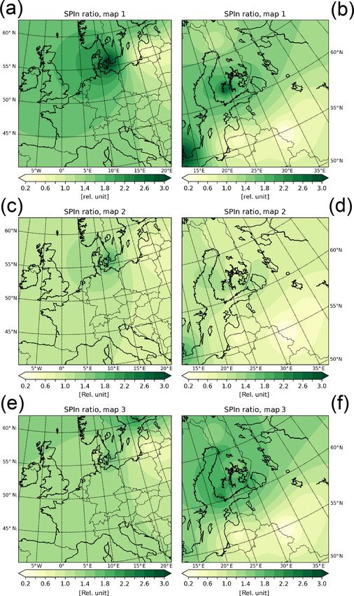
2100                                                        A. Kurganskiy et al.: Incorporation of pollen data in source maps

spring period (Sofiev et al., 2011). Such episodes can poten-       cupancy and climatic habitat quality maps for ragweed from
tially be described and forecast using atmospheric dispersion       an ecological model. The map covering Europe has been in-
models (Sofiev et al., 2006), helping sensitized individuals to     troduced to the atmospheric models as input data, run for
minimize their symptoms. Several European countries, such           several years and calibrated using pollen observation data.
as Denmark, have seen an increase in sensitized individuals         A birch pollen source map has been derived by Pauling et al.
over the past few decades (e.g. Rasmussen, 2002; Linneberg          (2012). The methodology includes using a forest inventory
et al., 2007). Generally, skin prick testing (SPT) is performed     combined with local and global land use datasets. The ob-
to identify sensitization of patients to common pollen aller-       tained map has been calibrated by observational pollen data
gens (e.g. Heinzerling et al., 2009). Haahtela et al. (2015)        and it covers Europe. An urban-scale grass pollen source in-
showed that the percentage of the population with positive          ventory has been obtained by Skjøth et al. (2013a) using GIS
SPT was about 35 % and 20 % in Finnish and Russian Kare-            and remote sensing data. A high-resolution (1 km) pollen
lia, respectively. These facts demonstrate the importance of        source inventory based on 12 taxa of trees, grass, and weeds
pollen studies using atmospheric dispersion models applied          has been produced by McInnes et al. (2017) for the UK to
for research and operational purposes (Klein et al., 2012).         be mainly used in exposure studies as well as other possi-
   A variety of pollen types are considered to be biological        ble applications. Many of these different pollen source maps
components by several atmospheric dispersion models such            show substantial variation, exemplified by the birch maps
as SILAM, COSMO-ART, WRF/CMAQ, Enviro-HIRLAM,                       over the UK produced by McInnes et al. (2017) and Pauling
and others (see e.g. Zink et al., 2012, 2013; Zhang et al.,         et al. (2012) or the European scale by comparing the maps
2014; Sofiev et al., 2015a; Baklanov et al., 2017; Sofiev,          by Pauling et al. (2012) with those by Siljamo et al. (2013).
2017; Zink et al., 2017). Information about distribution of         This suggests substantial disagreement or uncertainty in the
pollen sources, i.e. their presence and abundance in a re-          production of the pollen source maps – the key input data for
gion of study, plays a crucial role in aerobiological modelling     pollen dispersion models. An additional problem is the large
and forecasting using atmospheric dispersion models (e.g.           variability of the pollen production per plant in each specific
Zink et al., 2017). In other words, it is one of the key input      year. Several approaches have been proposed to address this
data used to simulate or forecast pollen emission, its atmo-        issue (e.g. Masaka and Maguchi, 2001; Ranta et al., 2005;
spheric transport, and depositions in these models. For this        Ritenberga et al., 2018).
reason, recent studies (e.g. Pauling et al., 2012; Bonini et al.,      Zink et al. (2017) applied an atmospheric dispersion model
2018) are devoted to developing pollen source inventories           to compare different ragweed pollen source maps using the
and maps. Two main approaches aiming to build/construct             COSMO-ART model. The results show that the pollen source
the pollen source inventories are suggested in the literature:      map resulting from combining land cover and pollen obser-
bottom-up and top-down (Skjøth et al., 2013b). The bottom-          vation data provides the best model performance. The ad-
up approach is based on statistical data of pollen source dis-      vantage of including a dispersion model is that, in principle,
tribution combined with land cover data obtained from re-           such models take into account atmospheric transport and its
mote sensing (Skjøth et al., 2008a). The limitation of this ap-     effect on pollen concentrations during a specific year (e.g.
proach is that statistical data are either unavailable or cover     Prank et al., 2013). A recent study showed high potential of
too large of a territory (e.g. the whole country) in some re-       extended four-dimensional variational data assimilation as a
gions. The top-down approach uses pollen observations as            rigorous procedure for obtaining the source maps’ calibra-
a starting point to estimate the abundance of different pollen      tions (Sofiev, 2019).
taxa and it can be combined with land use data and/or models           The literature review presented in this section shows there
for more detailed assessment of pollen sources on a regional        are multiple pollen source maps produced for different pollen
scale. Poor geographical and temporal coverage of the pollen        types and regions and using different approaches and data.
observation data can limit this approach in some regions.           Despite this, they are rarely applied to and intercompared us-
   Skjøth et al. (2008a) used the bottom-up approach to cre-        ing atmospheric dispersion models. This study aims to eval-
ate the Tree Species Inventory (TSI) for 39 species (including      uate three pollen source maps for the birch taxon using an
birch, oak, alder, etc.) redistributed to a 50 km grid to be used   atmospheric dispersion model and study the effect on the
in atmospheric dispersion models. The top-down approach             model results by combining these source maps with pollen
has been used to produce ragweed pollen inventories for the         data. The maps and model are described in the Methods sec-
Pannonian Basin (Skjøth et al., 2010), France (Thibaudon            tion below.
et al., 2014), Austria (Karrer et al., 2015), and Italy (Bonini
et al., 2018). The inventories are based on a combination
of pollen observation data, knowledge on ragweed ecology,
and detailed land cover information. The last (i.e. Bonini
et al., 2018) also includes influence of the Ophraella com-
muna beetle on the plants. Prank et al. (2013) as well as
Hamaoui-Laguel et al. (2015) have both used combined oc-

Atmos. Chem. Phys., 20, 2099–2121, 2020                                              www.atmos-chem-phys.net/20/2099/2020/
A. Kurganskiy et al.: Incorporation of pollen data in source maps                                                           2101

2     Methods                                                      cess: 23 January 2020) and National Forest Inventory (NFI)
                                                                   plot data as well as the NFI statistics (Brus et al., 2012).
2.1    Birch pollen source maps                                    Two techniques were used to derive the map: compositional
                                                                   kriging in areas with NFI plot data and regression modelling
Three birch pollen source maps have been chosen in this            outside of the areas. The National Forest Inventory statistics
study: (1) a map derived by combining land cover data and          were used to scale the regression model results. The map
forest inventory, (2) a map obtained from land cover data and      has 1 km horizontal resolution and covers most of Europe.
calibrated using model simulations and pollen observations,        However, information about birch pollen sources in Russia is
and (3) a statistical map resulting from analysis of forest in-    missing in Map 3. Therefore, the Russian sources were ex-
ventory and forest plot data (see Fig. A1 in the Appendix sec-     tracted from Map 1 and combined with Map 3 to fill the gap.
tion). The maps have been preprocessed for two modelling              The maps were introduced to Enviro-HIRLAM (Environ-
domains: P15 and T15. P15 covers part of Spain in the south        ment – High Resolution Limited Area Model) as input data
to part of Scandinavia in the north, with Denmark near the         to simulate birch pollen concentrations for the modelling do-
centre of the model domain (Fig. 1a). T15 covers Finland,          mains.
parts of Sweden, northwest Russia, the Baltic states, and Be-
larus (Fig. 1b).                                                   2.2   Model description
   Map 1 (see Fig. 2a, b) has been obtained by com-
bining three datasets: Global Land Cover Characteristics           Enviro-HIRLAM is an online coupled meteorology–
(GLCC, https://doi.org/10.5066/F7GB230D) version 2 (Bel-           chemistry model allowing us to take into account spatial–
ward et al., 1999), European Forest Institute tree cover (EFI;     temporal evolution of atmospheric chemical (Korsholm,
Päivinen et al., 2001), and Tree Species Inventory (TSI;           2009; Baklanov et al., 2017) and biological (Kurgan-
Skjøth et al. (2008a)). GLCC has global coverage and in-           skiy, 2017) aerosols simulated inside the meteorological
cludes geographical distribution of land cover, soil type, and     HIRLAM model (Undén et al., 2002). The current version
other various properties with 1 km horizontal resolution. EFI      of the Enviro-HIRLAM model is based on HIRLAM v7.2
covers Europe, has 1 km horizontal resolution, and contains        (https://hirlam.org). The detailed model description of all
spatial distribution of forest with subclasses, i.e. broadleaved   components can be found in Korsholm (2009), Kurganskiy
forest and coniferous forest. TSI is presented by 39 types of      (2017), and Baklanov et al. (2017) while this article is fo-
tree species (birch, oak, alder, etc.) and covers Europe with      cused on description of the Enviro-HIRLAM features rel-
50 km horizontal resolution and it is based on national forest     evant to pollen. In order to simulate birch pollen concen-
inventories and national statistics. The following layers have     trations, Enviro-HIRLAM requires external information/data
been extracted from these databases and combined to derive         on the spatial pollen source distribution and phenology, i.e.
the birch pollen source: land mask, forest, vegetation, urban      start of birch flowering, pollen production, characteristics of
territories (from GLCC), broadleaved forest (from EFI), and        pollen release (emissions) within the given study region, and
birch forest fraction in broadleaved forest (from TSI). For de-    where the spatial pollen source distribution is represented by
tails of the combining procedure see Kurganskiy et al. (2015)      the maps described above in Sect. 2.1. Atmospheric transport
and Kurganskiy (2017).                                             and dispersion as well as dry and wet depositions are calcu-
   Map 2 (see Fig. 2c, d) is a product of two datasets and         lated within Enviro-HIRLAM at each time step. In numeri-
a calibration using model simulations. The two datasets are        cal models, the start of birch pollen flowering is often deter-
EFI tree cover and ECOCLIMAP (Masson et al., 2003).                mined by applying simple crop growth models (e.g. McMas-
ECOCLIMAP is a global dataset with 1 km resolution and it          ter and Wilhelm, 1997); here the growing degree day (GDD)
includes 215 ecosystems. The model simulations have been           method is implemented in Enviro-HIRLAM. GDD is based
performed with the System for Integrated modeLing of At-           on accumulation of 2 m daily mean air temperatures above a
mospheric coMposition (SILAM, http://silam.fmi.fi, last ac-        given threshold (cut-off temperature) as this is the WMO def-
cess: 23 January 2020, Sofiev et al., 2015b) and pollen ob-        inition of GDD. It is assumed here that birch flowering starts
servation data for several years to ensure average unbiased        as soon as the accumulated temperature (GDD) reaches a cer-
representation of the Seasonal Pollen Integral (SPIn) with the     tain value depending on geographical location. These tem-
SILAM model, where SPIn is the integral of pollen concen-          perature sum threshold maps have been produced by Sofiev
trations over time (Galán et al., 2017). The calibrated map is     et al. (2013) and have been implemented and used as in-
calculated for a 1 km grid covering the whole of Europe with       put data for the GDD parameterization in Enviro-HIRLAM.
nearby regions. Details of the map calibration procedure are       The data were obtained by the fitting procedure applied using
described by Prank et al. (2013) using ragweed, and its appli-     the observed leaf unfolding dates (Siljamo et al., 2008) and
cation to birch in the SILAM model can be found in Sofiev          modelled ones by the GDD parameterization and ECMWF’s
(2017).                                                            ERA-40 reanalysis air temperature data (Uppala et al., 2005)
   Map 3 (see Fig. 2e, f) is the result of combining ICP-          utilized as input for GDD. It was shown in Kurganskiy
Level-I forest plot data (http://www.icp-forests.org, last ac-     (2017) that the temperature sum threshold maps are appli-

www.atmos-chem-phys.net/20/2099/2020/                                               Atmos. Chem. Phys., 20, 2099–2121, 2020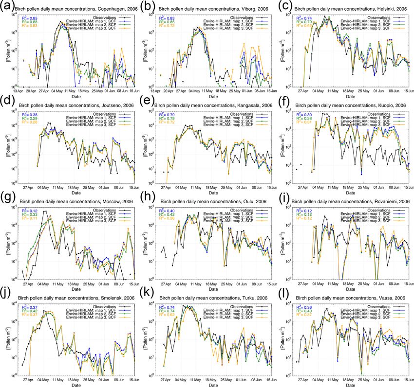
2102                                                          A. Kurganskiy et al.: Incorporation of pollen data in source maps

Figure 1. Location of the selected birch pollen observation sites with boundaries of the modelling domains: P15 (a) and T15 (b).

cable for use to simulate the birch flowering start in Enviro-          2.3   Model configuration
HIRLAM, even though another model (ERA-40) had been
originally used to obtain the maps. GDD is an integral part of          The Enviro-HIRLAM model is used to calculate pollen con-
Enviro-HIRLAM, and GDD calculations are performed for                   centrations in two different modelling domains shown in
the same dates as the model is run over. Birch pollen emis-             Fig. 1. Both domains have about 15 km horizontal resolu-
sion is meteorology-dependent and uses parameterizations                tion and 40 hybrid vertical levels. Input meteorological ini-
proposed by Sofiev et al. (2013). It is based on dimensionless          tial and boundary conditions were taken from the ECMWF
functions correcting the seasonal pollen productivity, here             IFS model (Persson, 2011) with 15 km resolution and 6 h in-
chosen to be 3.7×10⁸ pollen m−2 season−1 as a default value             tervals. The birch pollen emission module has the same set-
obtained for SILAM (Sofiev et al., 2013). The main meteo-               tings as described in Sofiev et al. (2013) and Siljamo (2013).
rological parameters affecting the emissions are air temper-            The Enviro-HIRLAM model was run from 1 March until
ature, relative humidity, wind speed, and accumulated pre-              15 June 2006 with the ECMWF input data covering the same
cipitation. The emitted birch pollen particles are subject to           period. The two model domains have been simulated with
atmospheric transport, which is parameterized in the same               three types of calculations: (1) a standard calculation, (2) a
way as for aerosols using the locally mass-conserving semi-             calculation that includes a correction for 2 m air temperature
Lagrangian (LMCSL) scheme (Kaas, 2008; Sørensen et al.,                 (T2 m ) bias between assimilated and simulated T2 m (termed
2013). The scheme provides proper mass conservation, shape              COR), and (3) a calculation that includes both the correc-
preservation, and multi-tracer efficiency required from a nu-           tion for temperature and a grid-based scaling factor for pollen
merical point of view. Dry deposition of birch pollen par-              emissions (termed SCF). These calculations were performed
ticles is determined by gravitational settling (Seinfeld and            using each of the selected pollen source maps, hence nine
Pandis, 2006). The gravitational settling parameterization is           model calculations for each of the two domains. The model
based on calculation of settling velocity according to Stokes           results from model simulations 2 and 3 are presented in the
law and taking into account density of birch pollen particles           Results section. The correction for T2 m bias is done in two
(800 kg m−3 ) and an estimated size of 22 µm (e.g. Mäkelä,              steps. Firstly, the model output from the simulations of type
1996) with near spherical shape (Sofiev et al., 2006). Wet              1 is used to calculate the biases (differences between sim-
deposition distinguishes between in-cloud (Stier et al., 2005)          ulated and assimilated T2 m ) for each assimilation window
and below-cloud (Baklanov and Sørensen, 2001) scavenging,               (i.e. 6 h). Secondly, the calculated biases are introduced in
i.e. removal of pollen particles from the atmosphere by pre-            the model simulations of type 2 (COR) where the simulated
cipitation. Both scavenging types are parameterized through             T2 m is corrected at each model time step using the average
the scavenging coefficients used for aerosol particles with             bias between the two nearest/closest assimilation windows.
r ≥ 10 µm.                                                              Further details of this procedure can be found in Kurganskiy
                                                                        (2017). The scaling factor for pollen emissions is based on
                                                                        the ratio between simulated and observed seasonal pollen in-
                                                                        tegral (SPIn) (see next section) from the simulations of type
                                                                        2 (COR). This provides 15 point values that have been in-

Atmos. Chem. Phys., 20, 2099–2121, 2020                                                   www.atmos-chem-phys.net/20/2099/2020/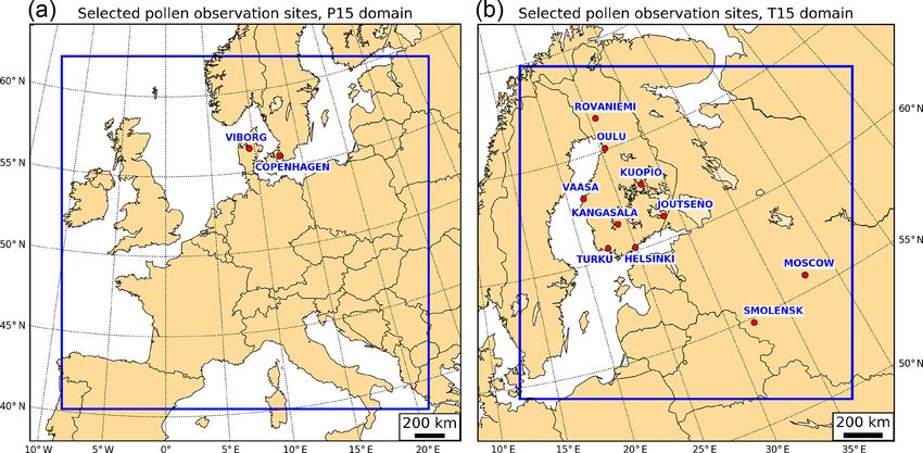
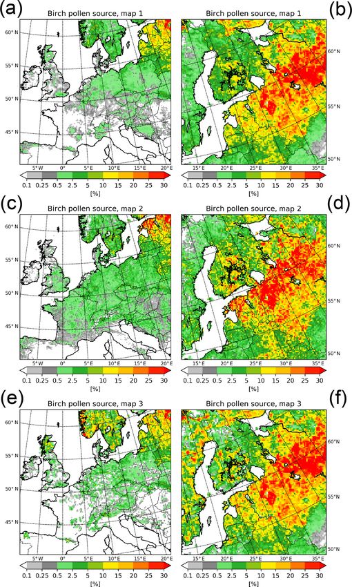
A. Kurganskiy et al.: Incorporation of pollen data in source maps                                                                     2103

Figure 2. Birch pollen source maps processed for two different modelling domains P15 (a, c, e) and T15 (b, d, f) with 15 km grid resolution.
Panels (a, b) correspond to Map 1, (c, d) to Map 2, and (e, f) to Map 3. The maps are shown as a percentage – the percentage cover of birch
in each 15 km × 15 km grid square.

www.atmos-chem-phys.net/20/2099/2020/                                                      Atmos. Chem. Phys., 20, 2099–2121, 2020
2104                                                      A. Kurganskiy et al.: Incorporation of pollen data in source maps

terpolated to the entire model domain, thereby providing a        culated according to Yu et al. (2006) since RMSE is highly
grid-based scaling factor for each of the tree source maps.       sensitive to outliers. The R 2 values are shown on the time
The interpolation procedure takes into account the weighted       series plots for each station, map, and run type as well as
distance between each observation point and grid cell with a      on the global scatter plots. The standard statistical metrics
constant radius of influence (1 km in this study). The proce-     have been calculated for the “main” pollen season (30 April–
dure also ensures the scaling factors are equal to around 1 in    15 June 2006) due to non-ergodicity (i.e. non-similarity in
the areas located far away from the observation points. This      space and time) and non-stationarity of the birch pollen time
is especially visible in P15 domain, e.g. in France (Fig. 3a,     series (Sofiev et al., 2015a). The threshold-based statistical
c, e). Further details of the interpolation procedure can be      approach (Siljamo et al., 2013) comprises calculations of the
found in Kurganskiy (2017). The grid-based scaling factor         model accuracy (MA), probability of detection (POD), false
has then been extracted for each model domain, thus pro-          alarm ratio (FAR), probability of false detection (POFD), and
viding six grid-based scaling factors (Fig. 3) applied for the    odds ratio (OR) using the threshold value for birch pollen
SCF simulations for all maps. The principal difference be-        concentrations Cth = 50 pollen m−3 . The threshold value Cth
tween the runs is that the COR runs include a constant value      is chosen since most of the population with pollen allergies
for birch pollen productivity (3.7×10⁸ pollen m−2 season−1 )      might start suffering from allergic reactions when daily mean
in each grid cell, whereas the productivity is calibrated using   birch pollen concentration C ≥ Cth in the air (Jantunen et al.,
the grid-based scaling factor (obtained from the COR runs         2012). Additionally, the modelled and observed birch pollen
and shown in Fig. 3) in the SCF runs. The model results           concentrations have been sorted into classes in order to es-
were compared with the pollen observation data at 12 mea-         timate the number of cases for low (1–10 pollen m−3 ), mod-
surement sites located in Finland, Denmark, and Russia (see       erate (10–100 pollen m−3 ), high (100–1000 pollen m−3 ), and
Fig. 1) for all model runs.                                       very high (> 1000 pollen m−3 ) birch pollen concentrations.
                                                                  The sorted data plotted with corresponding standard errors
2.4    Used observations and statistical evaluation of            are shown in the Results section. Hit rates (HRs) are calcu-
       model results                                              lated for the classes, and their results are shown in tables in
                                                                  the Results section. The results of the statistical significance
Daily concentrations of birch pollen were used from 12 sites      test (chi-squared test) performed for the HR values are also
(Fig. 1a, b), and furthermore annual SPIn values were ob-         discussed. For summary of the thresholds, classes, and met-
tained from three additional sites in Lithuania, published        rics used to calculate the threshold-based statistics, the reader
by Veriankaite (2010), in order to strengthen the calcula-        is referred to Tables A5–A6 in the Appendix section.
tion of the grid-based scaling factor (Sect. 2.3). The obser-
vational data were obtained using 7 d volumetric samplers
(Hirst, 1952) and analysed according to standard methods          3   Results
in aerobiology (Galán et al., 2014). Station names and co-
ordinates are presented in the Appendix section along with        The simulated time series of birch pollen concentrations have
statistical summaries for each station (see Tables A1–A4),        been compared to the selected pollen observation sites by de-
while overall results are presented in the Results section. The   termining the start and end of the birch pollen season and
statistical evaluation includes standard and threshold-based      applying the standard statistics as well as threshold-based
statistical approaches, e.g. previously used by Siljamo et al.    statistics described in the Methods section. The modelled and
(2013) and Sofiev et al. (2015a) and calculated in this pa-       observed time series are also shown in Figs. 4–5 for COR and
per for each map (1, 2, 3) and run (COR, SCF) type. The           SCF runs, respectively. The start of the birch pollen season
start and end of the birch pollen season are calculated us-       is simulated quite well for both runs and all maps. Station-
ing the retrospective method according to Nilsson and Pers-       wise the bias does not exceed 2–3 d at all stations and indi-
son (1981), here defined as the dates when the total sums         cates 2 d too early flowering on average for all maps. Simu-
of birch pollen concentrations (SPIn) reach 5 % and 95 %,         lation of the last flowering day turns out to be the most chal-
correspondingly. The criteria are chosen to provide filtration    lenging for Enviro-HIRLAM. The bias shows too late flow-
of LRT (long-range-transport) episodes which have a signif-       ering at almost all stations. On average, it varies from 15 d
icant impact in northern Europe, especially in the beginning      (Map 3) to 9 d (Map 2) according to the COR run. Rescal-
of the birch pollen season (Ranta et al., 2006; Skjøth et al.,    ing of the pollen productivity (SCF run) reduced the bias by
2007; Mahura et al., 2007; Veriankaite, 2010). The standard       2–3 d for each map. The largest biases for the last flowering
statistical approach includes calculations of correlation co-     day are found at five Finnish sites (Helsinki, Joutseno, Kan-
efficient (R), coefficient of determination (R 2 ), mean bias     gasala, Vaasa, and Kuopio) and two Russian sites (Moscow
(MB), and root-mean-square error (RMSE), and the evalu-           and Smolensk), and they are related to overestimation of the
ation primarily concerns correlation and RMSE. Two addi-          observed birch pollen concentrations at the end of the season
tional metrics, normalized mean bias factor (NMBF) and nor-       for both COR and SCF runs (see Figs. 4 and 5). It can be
malized mean absolute error factor (NMAEF), are also cal-         addressed to large variations in the year-to-year pollen pro-

Atmos. Chem. Phys., 20, 2099–2121, 2020                                            www.atmos-chem-phys.net/20/2099/2020/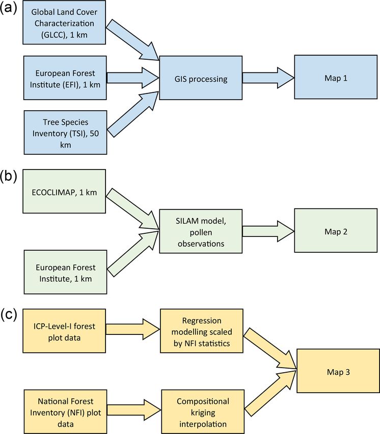
A. Kurganskiy et al.: Incorporation of pollen data in source maps                                                                         2105

Figure 3. SPIn ratio used to calibrate pollen productivity in the SCF runs for two different domains P15 (a, c, e) and T15 (b, d, f). Panels (a,
b) correspond to Map 1, (c, d) to Map 2, and (e, f) to Map 3.

www.atmos-chem-phys.net/20/2099/2020/                                                        Atmos. Chem. Phys., 20, 2099–2121, 2020
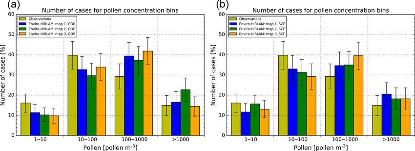
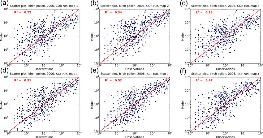
2106                                                       A. Kurganskiy et al.: Incorporation of pollen data in source maps

duction in that region which, in turn, introduce a large bias in   ceed 7 %. The model accuracy (MA) – the fraction of correct
the model simulations.                                             simulations – is higher than 70 % for all model simulations.
   Generally, the time series of the modelled birch pollen         The POD values show that the Enviro-HIRLAM model sim-
concentrations (Figs. 4 and 5) show good agreement with            ulates the high concentrations (> 50 pollen m−3 ) correctly in
observations for all maps at most of the selected stations. The    more than 70 % of cases. The fraction of incorrect simula-
COR run indicates that the model behaves similarly with re-        tions for the high concentrations (FAR values) is less than
spect to describing variance in observations (see R 2 values       30 % for the model setups. The POFD values show that the
in Fig. 4), except for some stations (e.g. Moscow, Helsinki)       fraction of the cases when concentrations are simulated as
where Map 2 provides higher R 2 values in comparison with          high but observed as low (i.e. < 50 pollen m−3 ) is more than
Map 1 and Map 3. The SCF run did not affect the R 2 values         30 % for the COR runs, and it decreases below 30 % after
significantly, but it reduced the mean bias (MB, NMBF) at          rescaling of the pollen productivity (SCF run). As expected
the stations (see Tables A1–A4). The highest R 2 values are        the odds ratio (OD) values increase in the SCF run for all
found at two Danish sites (Copenhagen and Viborg) where            maps. The modelled and observed birch pollen concentra-
the model explains more than 70 % of variance found in ob-         tions have been grouped in order to estimate the number of
servations for all considered maps and model runs. It should       cases for low, moderate, high, and very high birch pollen con-
be noted here that the R 2 values decrease slightly at the Dan-    centrations (see Fig. 7). As can be seen, the Enviro-HIRLAM
ish sites according to the SCF runs. The reason for this is that   model simulates the low and very high pollen concentrations
the simulated concentrations in the SCF runs are increased         quite well with a difference less than ±5 % between the mod-
almost every single day, which has the effect of reducing the      elled and observed number of cases for both COR (Fig. 7a)
underestimation found in the central season (e.g. Fig. 5a) and     and SCF (Fig. 7b) runs and all maps. The largest differences
increasing LRT, most likely originating from sources found         between the modelled and observed number of cases are
in Germany and Poland at the beginning of the season and           found for the moderate and high pollen concentrations, but
from Scandinavia at the end of the season. For more detailed       the differences are within the error bars (see Fig. 7). Map 2
statistical summaries at the stations, the reader is referred to   underestimates the number of cases for the moderate con-
tables in the Appendix section.                                    centrations by 10 %, whereas Map 3 overestimates the high
   The global standard statistical metrics for all stations are    ones by more than 10 % (COR run). The SCF run slightly
presented in Table 1. According to the COR run the model           improves the results for the moderate and high number of
performs slightly better with Map 2. It is supported by a          cases.
higher correlation coefficient (R = 0.59) and lower mean              The HR calculations (see Tables 3–4) show that simula-
bias (MB = 69.08 pollen m−3 , NMBF = 0.09) in comparison           tions of the moderate and high birch pollen concentrations
with two other maps. One can assume that this result should        are the most challenging for all model setups. The SCF run
be expected since pollen observations are already included         (Table 4) indicates improvements of the model score for the
in the methodology used to obtain Map 2. Rescaling of the          moderate and high birch pollen concentrations. However, the
pollen productivity (SCF run) provides improvement of the          hit rates still do not exceed 50 % for all maps. This feature
Enviro-HIRLAM model performance by increasing the R                is also visible on the scatter plots in Fig. 6. The HR values
values (R = 0.72 for Maps 1 and 2 and R = 0.68 for Map 3)          for the low pollen concentrations are quite high and exceed
and decreasing the MB, NMBF, and NMAEF values. How-                90 % for COR and 80 % for SCF runs. The very high pollen
ever, RMSE is large (i.e. > 1000 pollen m−3 ) for all maps         concentrations are simulated slightly better by using Map 3
and both model runs. It can be explained by sensitivity of         with HR = 70 %. However, according to the chi-square test
RMSE to large differences between modelled and observed            the differences between the HR values for different maps are
values. The large bias for the last flowering day simulation       not statistically significant for both COR and SCF runs.
contributes significantly to the RMSE values.
   The global scatter plots (Fig. 6) also indicate improve-
ments in the modelled–observed concentration agreement             4   Discussion
expressed as an increase in the R 2 for the SCF model setup.
As seen, the coefficients of determination do not exceed 0.34      Analysis of the start of birch pollen season showed good
(Map 2) for all maps in the COR run. The SCF run provides          model performance for all maps with the bias not exceed-
R 2 values around 0.5 for all maps. This means that the model      ing 2 d on average. Such error is acceptable by state-of-the-
can explain about 50 % of variance found in observations af-       art atmospheric dispersion models (e.g. Sofiev et al., 2015a).
ter the rescaling using any of the maps.                           The analysis did not reveal significant dependency of the start
   The threshold-based statistical metrics calculated for each     of the birch pollen season on the underlying pollen source
map and model run are shown in Table 2. The results indicate       map and/or pollen productivity. This could be explained by
similar behaviour of the model when comparing performance          the fact that the start of the birch pollen season is calculated
of the maps. The values of the statistical metrics are slightly    using meteorological parameters (i.e. temperate sum thresh-
different between the maps, but the difference does not ex-        olds) employed in GDD parameterization in the model. How-

Atmos. Chem. Phys., 20, 2099–2121, 2020                                             www.atmos-chem-phys.net/20/2099/2020/
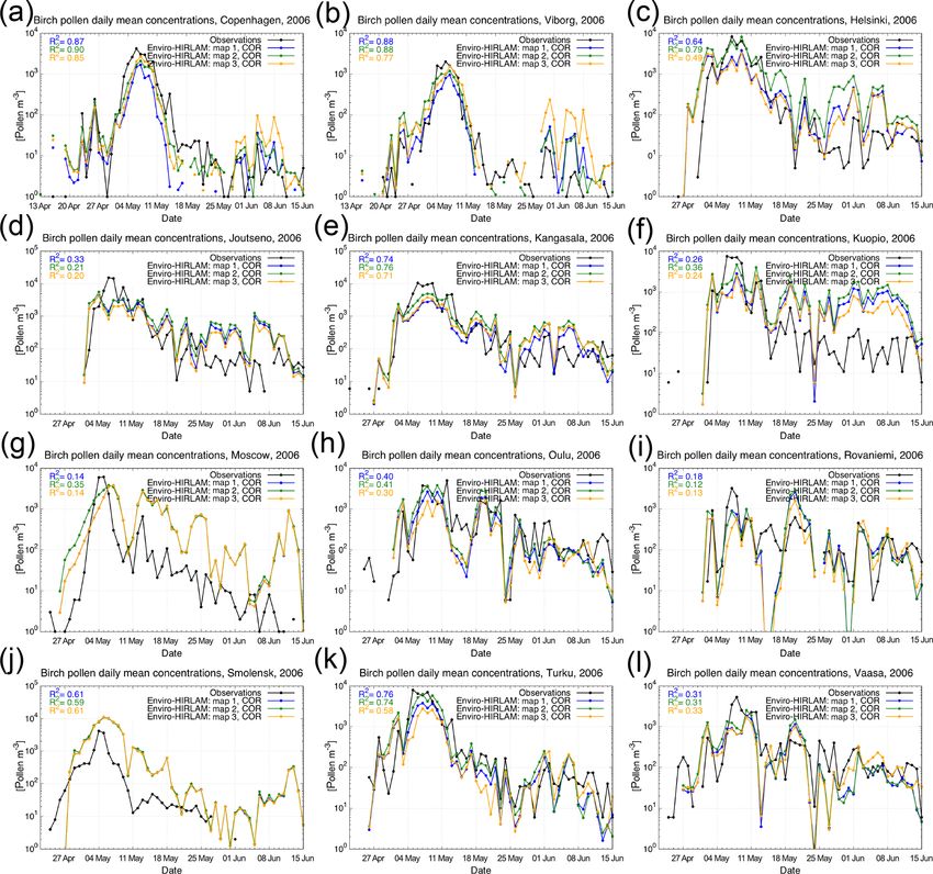
A. Kurganskiy et al.: Incorporation of pollen data in source maps                                                                 2107

Figure 4. Time series of the modelled and observed birch pollen daily mean concentrations for the selected pollen observation sites. The
modelled concentrations correspond to each simulated map according to the COR run. A base-10 log scale is used for the y axis.

ever, long-distance transport of birch pollen has often been          suggestion from other studies that long-distance transport of
observed in that region (e.g. Hjelmroos, 1992; Mahura et al.,         pollen is an episodic phenomenon (e.g. Smith et al., 2008;
2007), which can systematically affect the start of the pollen        Fernández-Rodríguez et al., 2014) and that the overall con-
season (Skjøth et al., 2007). It could therefore be assumed           tribution to locally observed birch pollen concentration is due
that changing the source term in remote regions such as               to sources found within the region (Sofiev, 2017). Add to this
Poland could affect the start of the calculated pollen season in      that urban areas have previously been identified as areas that
Denmark and Sweden. This phenomenon was not observed,                 may enhance pollen production of flowering plants (Ziska
which may be explained by the fact that the scaling factor for        et al., 2003). This may be particularly relevant for Copen-
Poland was near unity for all three maps, while the scaling           hagen as a substantial fraction of the birch pollen observed
factor for Copenhagen and the close surroundings was sub-             is expected to originate from a source found in the city itself
stantially higher. This observation therefore complements the         (Skjøth et al., 2008b). The last flowering day simulation was

www.atmos-chem-phys.net/20/2099/2020/                                                   Atmos. Chem. Phys., 20, 2099–2121, 2020
2108                                                        A. Kurganskiy et al.: Incorporation of pollen data in source maps

Figure 5. Time series of the modelled and observed birch pollen daily mean concentrations for the selected pollen observation sites. The
modelled concentrations correspond to each simulated map according to the SCF run. A base-10 log scale is used for the y axis.

the most challenging for Enviro-HIRLAM. Map 2 showed                  is that the large pollen emission area found in Russia, north
the lowest bias estimated as 6 d (delay of end of flowering)          of Moscow and Smolensk, is overestimated for this partic-
on average for the stations according to the SCF runs. How-           ular year. The source is found in all three source maps and
ever, such bias is a known feature for state-of-the-art atmo-         the overestimation is further supported by the fact that the
spheric models (e.g. Sofiev et al., 2015a). Introducing more          model simulates large amounts of birch pollen concentration
pollen observation stations and performing more iterations            very late in the season at Moscow and Smolensk (Fig. 4g
for rescaling of pollen emissions (i.e. repeating SCF runs            and j), most likely originating from more northerly regions.
several times) would strengthen the current approach, and it          This area will occasionally also affect the Finnish stations
could potentially improve the modelling of the last flowering         as it is well known that this region receives LRT from Rus-
day. Station-wise the Finnish and Russian sites had bias ≥ 2          sia (e.g. Sofiev et al., 2006). The study therefore comple-
weeks in all model runs. One of the possible reasons for this         ments a multi-model ensemble that demonstrated generally

Atmos. Chem. Phys., 20, 2099–2121, 2020                                                 www.atmos-chem-phys.net/20/2099/2020/
A. Kurganskiy et al.: Incorporation of pollen data in source maps                                                                       2109

Table 1. Global “standard” statistical metrics obtained by comparing the modelled (Cm ) and observed (Co ) daily mean birch pollen concen-
trations. The metrics were calculated using all available station data for both simulated domains, over the 30 April–15 June 2006 period. Cm ,
Co , MB, and RMSE are given (pollen m−3 ). The results were statistically significant for all maps (p value < 0.01 according to a Student’s
t test).

                         Run                R       Cm          Co         MB      RMSE       NMBF      NMAEF
                         COR, Map 1      0.47    545.89    683.63     −137.74     1587.81     −0.25          1.12
                         COR, Map 2      0.59    752.71    683.63       69.08     1465.79      0.09          0.81
                         COR, Map 3      0.42    509.49    683.63     −174.14     1639.47     −0.34          1.21
                         SCF, Map 1      0.72    661.64    683.63      −21.99     1229.16     −0.03          0.77
                         SCF, Map 2      0.72    630.02    683.63      −53.61     1223.95     −0.09          0.76
                         SCF, Map 3      0.68    614.41    683.63      −69.22     1290.04     −0.10          0.75

Figure 6. Scatter plots for birch pollen concentrations when comparing COR (a–c) and SCF (d–f) model runs with observations for Map 1 (a,
d), Map 2 (b, e), and Map 3 (c, f).

                                                                         good results for Europe and also highlighted that large vari-
                                                                         ations in the year-to-year pollen production in that region
Table 2. The threshold-based statistical metrics obtained by com-        can introduce a large bias in the model simulations (Sofiev
paring model simulations with observed daily mean concentrations.        et al., 2015a). Large annual variations in the birch pollen in-
MA, POD, FAR, and POFD are given as a percentage.                        tegral are well known for a number of European countries
                                                                         (Latałowa et al., 2002; Dahl et al., 2013; Piotrowska and
      Run, map         MA      POD     FAR      POFD      OR             Kaszewski, 2011), as these annual fluctuations are generally
      COR, Map 1       76.3    74.6    25.4      31.9     2.3            not accounted for in the atmospheric models (e.g. Ritenberga
      COR, Map 2       74.7    71.1    28.9      38.3     1.9            et al., 2018).
      COR, Map 3       75.4    72.7    27.3      35.0     2.1               The standard statistical metrics indicated a slightly better
      SCF, Map 1       79.5    77.7    22.3      27.6     2.8            performance of the Enviro-HIRLAM with Map 2 on average
      SCF, Map 2       79.8    79.1    20.9      24.8     3.2            for the stations according to the COR run. However, even
      SCF, Map 3       79.7    77.1    22.9      29.1     2.7            for this map, the model explained less than 35 % of vari-
                                                                         ance in observations. It is therefore plausible to attribute the
                                                                         remaining part of the disagreement to small-scale patterns

www.atmos-chem-phys.net/20/2099/2020/                                                       Atmos. Chem. Phys., 20, 2099–2121, 2020
2110 A. Kurganskiy et al.: Incorporation of pollen data in source maps Figure 7. Histogram of the observed and modelled birch pollen concentrations sorted into low (1–10 pollen m−3 ), moderate (10– 100) pollen m−3 , high (100–1000 pollen m−3 ), and very high (> 1000 pollen m−3 ) classes. Panel (a) corresponds to COR and (b) to the SCF model simulations. of the birch habitation, which are neither captured by ex- of the moderate and high birch pollen concentrations ap- isting calibration methods nor satisfactorily reproduced by peared to be the most challenging for Enviro-HIRLAM for the land cover datasets. In this study, a scaling of the pollen all maps. The hit rates were less than 50 % for all model se- productivity improved the model results significantly for all tups. This reveals a need for improvement of the rescaling of source terms and provided near-identical results for Map 1 birch pollen productivity by introducing more observational and Map 2. The small-scale pattern in birch habitation will points, in particular in areas sparse with data or regions with be difficult to capture by the land cover datasets, which will high emissions such as parts of Russia, and/or performing have the effect that a small but diffuse emission source found more iterations. The differences of the HR values appeared in many locations is not present, causing the model to un- to be not significant during inter-comparison of the maps. derestimate medium concentration levels. Conversely, the This study concerning birch pollen complements other stud- large emission source found in parts of Russia will cause the ies on ragweed (Prank et al., 2013; Hamaoui-Laguel et al., model to overestimate periods when long-distance transport 2015), which also demonstrated the need for recalibration of is present. This effect of over- and underestimation will vary the source term. However, it has since been shown by Zink from year to year, depending on pollen productivity, which is et al. (2017) that source terms combining pollen data from known to vary from year to year and between regions (Ranta several years with detailed land cover data can outperform et al., 2005). This suggests that accurate exposure calcula- other approaches minimizing the need for local calibrations. tions that use dispersion models should preferably use data This approach is also limited by the fact that only a few re- fusion that combines a detailed inventory-based source term gions have a sufficiently high number of pollen observations (e.g. Skjøth et al., 2008a; Pekkarinen et al., 2009; Sofiev, (Zink et al., 2017). Furthermore, abrupt annual changes in 2017) along with observed pollen concentrations covering the underlying pollen integral can be caused by changes in the period of interest. Other possible sources of error (e.g. the pollen emission (Bonini et al., 2015; Bonini et al., 2018). timing of pollen release, quality of meteorological parame- The insufficient density of the observational network also ters, simulation of atmospheric transport and removal pro- became the methodological limitation of the current study: cesses) could also be taken into account. However, their ef- we have used the same data from the same stations and for fect is less important in comparison with the quality of emis- the same years for both calibration and evaluation. However, sion (source) maps – the main uncertainty in air pollution and we separated them frequency-wise: calibration uses the an- pollen dispersion modelling. nual or multi-annual average whereas the evaluation primar- The threshold-based statistics calculated relative to one ily concerned correlation and RMSE. It should be noted that threshold value (Cth = 50 pollen m−3 ) showed a good model an independent evaluation that does not use pollen data is agreement with observations independently of the map used. shown by analysis of the COR runs in the study. Another The threshold-based analysis was also carried out for low (1– approach could be to carry out a cross-validation procedure 10 pollen m−3 ), moderate (10–100 pollen m−3 ), high (100– using the so-called leave-one-out procedure as this tests the 1000 pollen m−3 ), and very high (> 1000 pollen m−3 ) birch sensitivity of individual data points. However, such a sensi- pollen concentrations. According to the analysis, simulations tivity study requires 15 additional model simulations for each Atmos. Chem. Phys., 20, 2099–2121, 2020 www.atmos-chem-phys.net/20/2099/2020/
A. Kurganskiy et al.: Incorporation of pollen data in source maps                                                            2111

                                                                    map and each modelling domain, hence 90 simulations. The
                                                                    increased computational cost makes this exercise unfeasible,
Table 3. Hit rates of the Enviro-HIRLAM birch pollen simulations
                                                                    suggesting that other approaches need to be developed.
(COR run) for the classes
zero or low, moderate, high, and very high. The classes are based
on daily mean pollen concentrations (pollen m−3 ).                  5   Conclusions
    Observation      0–10    10–100     100–1000    > 1000          The aim of the study was to evaluate three birch pollen
    model                                                           source maps using the atmospheric dispersion model Enviro-
    COR run, Map 1                                                  HIRLAM. The evaluation has been performed for 12 pollen
                                                                    observation sites located in Denmark, Finland, and Russia.
    0–10           94.5 %      4.6 %        0.9 %     0.0 %
                                                                    The modelled and observed time series of birch pollen con-
    10–100         29.1 %     46.0 %       24.9 %     0.0 %
                                                                    centrations have been analysed for the start and end of flow-
    100–1000        6.1 %     41.3 %       38.5 %    14.1 %
    > 1000          0.0 %     11.5 %       25.3 %    63.2 %         ering as well as by calculating the standard and threshold-
                                                                    based statistical metrics for two sets of the Enviro-HIRLAM
    COR run, Map 2                                                  model runs: without and with calibration using pollen obser-
    0–10           95.2 %      3.9 %        0.9 %     0.0 %         vations.
    10–100         29.0 %     47.9 %       23.1 %     0.0 %            The analysis did not reveal significant dependency of the
    100–1000        9.2 %     44.4 %       37.7 %     8.7 %         start–end of the birch pollen season on the underlying pollen
    > 1000          0.0 %     15.1 %       28.6 %    56.3 %         source map. The statistical analysis showed a good model
    COR run, Map 3                                                  agreement with the observed birch pollen concentrations in
                                                                    the region studied. The model can explain up to 50 % of
    0–10           95.0 %      4.2 %        0.8 %     0.0 %         variance found in observations after the calibration with all
    10–100         34.0 %     44.2 %       21.8 %     0.0 %         maps. It was shown that the remaining part of the disagree-
    100–1000        6.9 %     40.5 %       40.1 %    12.5 %
                                                                    ment should be attributed to small-scale patterns of the birch
    > 1000          0.0 %     10.0 %       20.0 %    70.0 %
                                                                    habitation, which are neither captured by existing calibra-
                                                                    tion methods nor satisfactorily reproduced by the land cover
                                                                    datasets. The analysis also revealed that the insufficient den-
                                                                    sity of the observational network was the methodological
                                                                    limitation of the study.
Table 4. Hit rates of the Enviro-HIRLAM birch pollen simulations       Generally, it was shown that calibration of the maps using
(SCF run) for the classes zero or low, moderate, high, and very     pollen observations covering the investigation year signifi-
high. The classes are based on daily mean pollen concentrations     cantly improved the model performance for all three maps.
(pollen m−3 ).                                                      The findings also indicate the large sensitivity of the model
                                                                    results to the source maps and agree well with other studies
    Observation      0–10    10–100     100–1000    > 1000          on birch showing that pollen or hybrid-based source maps
    model
                                                                    provide the best model performance. This study highlights
    SCF run, Map 1                                                  the importance of including pollen data in the production of
                                                                    source maps for pollen dispersion modelling and for expo-
    0–10           85.5 %    12.1 %       2.4 %      0.0 %
    10–100         32.0 %    49.5 %      18.5 %      0.0 %          sure studies.
    100–1000       5.3 %     40.0 %      46.8 %      7.9 %
    > 1000          0.0 %    12.7 %      23.6 %      63.7 %
    SCF run, Map 2
    0–10           84.8 %    13.2 %       2.0 %      0.0 %
    10–100         29.6 %    48.5 %      21.9 %      0.0 %
    100–1000       5.7 %     41.8 %      46.3 %      6.2 %
    > 1000          0.0 %    11.4 %      23.7 %      64.9 %
    SCF run, Map 3
    0–10           84.0 %    14.3 %       1.7 %      0.0 %
    10–100         34.9 %    46.3 %      18.8 %      0.0 %
    100–1000       6.4 %     42.7 %      44.0 %      6.9 %
    > 1000          0.0 %     5.1 %      24.2 %      70.7 %

www.atmos-chem-phys.net/20/2099/2020/                                                Atmos. Chem. Phys., 20, 2099–2121, 2020
2112 A. Kurganskiy et al.: Incorporation of pollen data in source maps Appendix A Figure A1. Flowcharts outlining the data and methods used to ob- tain Map 1 (a), Map 2 (b), and Map 3 (c). Atmos. Chem. Phys., 20, 2099–2121, 2020 www.atmos-chem-phys.net/20/2099/2020/
A. Kurganskiy et al.: Incorporation of pollen data in source maps                                                                      2113

Table A1. Birch pollen statistical metrics for the selected observation sites: COR run. Cm , Co , MB, and RMSE are in pollen per cubic metre;
p value < 0.05.

         Site name     Map       Lat         Long           R         Cm          Co         MB       RMSE      NMBF       NMAEF
         Helsinki                60.17◦ N    24.90◦ E
                       Map 1                             0.80     574.69      879.28    −299.59      1269.56     −0.53         1.05
                       Map 2                             0.89    1233.00      879.28     353.72       895.53      0.40         0.64
                       Map 3                             0.70     515.97      879.28    −363.31      1412.44     −0.70         1.28
         Joutseno                61.10◦ N    28.50◦ E
                       Map 1                             0.57     838.61     1345.81     −507.2      2865.20     −0.60         1.30
                       Map 2                             0.46    1002.84     1345.81    −342.97      2945.21     −0.34         1.21
                       Map 3                             0.45     659.18     1345.81    −686.63      3070.78     −1.04         1.71
         Kangasala               61.47◦ N    24.08◦ E
                       Map 1                             0.86     569.86     1442.55    −872.69      2369.17     −1.53         1.80
                       Map 2                             0.87    1018.23     1442.55    −424.32      1841.15     −0.42         0.87
                       Map 3                             0.84     701.75     1442.55     −740.8      2252.54     −1.06         1.46
         Kuopio                  62.88◦ N    27.63◦ E
                       Map 1                             0.51     672.75      777.23    −104.48      1627.23     −0.16         1.28
                       Map 2                             0.60    1032.18      777.23     254.95      1508.64      0.33         1.25
                       Map 3                             0.49     530.67      777.23    −246.56      1665.51     −0.46         1.45
         Oulu                    65.07◦ N    25.52◦ E
                       Map 1                             0.63     469.77      682.43    −212.66       845.99     −0.45         0.85
                       Map 2                             0.64     686.56      682.43       4.13       883.44      0.01         0.67
                       Map 3                             0.55     333.85      682.43    −348.58       950.66     −1.04         1.33
         Rovaniemi               66.55◦ N    25.73◦ E
                       Map 1                             0.42     302.92      309.64       −6.72      574.93     −0.02         0.92
                       Map 2                             0.35     324.04      309.64       14.40      646.57      0.05         0.98
                       Map 3                             0.36     211.50      309.64      −98.14      544.39     −0.46         1.14

www.atmos-chem-phys.net/20/2099/2020/                                                      Atmos. Chem. Phys., 20, 2099–2121, 2020
2114 A. Kurganskiy et al.: Incorporation of pollen data in source maps
Table A2. Birch pollen statistical metrics for the selected observation sites: COR run. Cm , Co , MB, and RMSE are in pollen per cubic metre;
p value < 0.05.
Site name Map Lat Long R Cm Co MB RMSE NMBF NMAEF
Turku 60.53◦ N 22.47◦ E
Map 1 0.87 548.80 925.02 −376.22 1269.02 −0.69 0.89
Map 2 0.86 862.73 925.02 −62.29 1011.47 −0.07 0.50
Map 3 0.76 404.71 925.02 −520.31 1605.97 −1.29 1.58
Vaasa 63.10◦ N 21.62◦ E
Map 1 0.56 307.10 548.43 −241.33 902.99 −0.79 1.24
Map 2 0.56 389.07 548.43 −159.36 871.11 −0.41 1.06
Map 3 0.57 294.52 548.43 −253.91 913.76 −0.86 1.29
Moscow 55.74◦ N 37.55◦ E
Map 1 0.37 647.42 388.28 259.14 1269.87 0.67 1.74
Map 2 0.59 733.42 388.28 345.14 1100.18 0.89 1.65
Map 3 0.37 647.40 388.28 259.12 1270.04 0.67 1.74
Smolensk 54.78◦ N 32.05◦ E
Map 1 0.78 1382.37 259.32 1123.05 2542.82 4.33 4.33
Map 2 0.77 1368.29 259.32 1108.97 2466.38 4.28 4.28
Map 3 0.78 1377.17 259.32 1117.85 2537.15 4.31 4.31
Copenhagen 55.72◦ N 12.57◦ E
Map 1 0.93 144.63 445.83 −301.2 717.53 −2.08 2.10
Map 2 0.95 231.68 445.83 −214.15 560.20 −0.92 0.95
Map 3 0.92 263.55 445.83 −182.28 503.85 −0.69 0.79
Viborg 56.45◦ N 9.40◦ E
Map 1 0.94 91.72 199.70 −107.98 325.90 −1.18 1.34
Map 2 0.94 150.53 199.70 −49.17 229.32 −0.33 0.64
Map 3 0.88 173.58 199.70 −26.12 251.93 −0.15 0.58
Atmos. Chem. Phys., 20, 2099–2121, 2020 www.atmos-chem-phys.net/20/2099/2020/A. Kurganskiy et al.: Incorporation of pollen data in source maps 2115
Table A3. Birch pollen statistical metrics for the selected observation sites: SCF run. Cm , Co , MB, and RMSE are in pollen per cubic metre;
p value < 0.05.
Site name Map Lat Long R Cm Co MB RMSE NMBF NMAEF
Helsinki 60.17◦ N 24.90◦ E
Map 1 0.86 841.46 879.28 −37.82 942.66 −0.04 0.55
Map 2 0.89 981.76 879.28 102.48 833.56 0.12 0.51
Map 3 0.79 785.22 879.28 −94.06 1122.77 −0.12 0.68
Joutseno 61.10◦ N 28.50◦ E
Map 1 0.62 1224.33 1345.81 −121.48 2601.02 −0.10 0.92
Map 2 0.54 989.56 1345.81 −356.25 2823.36 −0.36 1.15
Map 3 0.53 1015.47 1345.81 −330.34 2812.42 −0.33 1.12
Kangasala 61.47◦ N 24.08◦ E
Map 1 0.89 1100.24 1442.55 −342.31 1595.21 −0.31 0.73
Map 2 0.89 1135.93 1442.55 −306.62 1575.66 −0.27 0.69
Map 3 0.85 1200.14 1442.55 −242.41 1633.02 −0.20 0.72
Kuopio 62.88◦ N 27.63◦ E
Map 1 0.55 953.83 777.23 176.6 1559.38 0.23 1.23
Map 2 0.62 817.90 777.23 40.67 1474.81 0.05 1.07
Map 3 0.56 755.99 777.23 −21.24 1543.05 −0.03 1.09
Oulu 65.07◦ N 25.52◦ E
Map 1 0.63 669.43 682.43 −13.00 876.15 −0.02 0.68
Map 2 0.65 676.29 682.43 −6.14 861.12 −0.01 0.66
Map 3 0.60 583.34 682.43 −99.09 857.18 −0.17 0.78
Rovaniemi 66.55◦ N 25.73◦ E
Map 1 0.35 368.22 309.64 58.58 691.80 0.19 1.06
Map 2 0.34 309.19 309.64 −0.45 632.14 0.00 0.97
Map 3 0.34 332.60 309.64 22.96 611.50 0.07 0.98
www.atmos-chem-phys.net/20/2099/2020/ Atmos. Chem. Phys., 20, 2099–2121, 20202116 A. Kurganskiy et al.: Incorporation of pollen data in source maps
Table A4. Birch pollen statistical metrics for the selected observation sites: SCF run. Cm , Co , MB, and RMSE are in pollen per cubic metre;
p value < 0.05.
Site name Map Lat Long R Cm Co MB RMSE NMBF NMAEF
Turku 60.53◦ N 22.47◦ E
Map 1 0.86 958.24 925.02 33.22 1032.33 0.04 0.49
Map 2 0.86 924.51 925.02 −0.51 1033.30 0.00 0.49
Map 3 0.79 732.00 925.02 −193.02 1241.52 −0.26 0.66
Vaasa 63.10◦ N 21.62◦ E
Map 1 0.60 507.24 548.43 −41.19 831.66 −0.08 0.84
Map 2 0.63 475.72 548.43 −72.71 811.14 −0.15 0.86
Map 3 0.61 503.97 548.43 −44.46 817.61 −0.09 0.82
Moscow 55.74◦ N 37.55◦ E
Map 1 0.34 392.03 388.28 0.01 1206.26 0.01 1.25
Map 2 0.57 334.68 388.28 −0.16 1047.91 −0.16 1.18
Map 3 0.33 375.92 388.28 −0.03 1208.18 −0.03 1.28
Smolensk 54.78◦ N 32.05◦ E
Map 1 0.61 505.21 259.32 245.89 859.77 0.95 1.34
Map 2 0.65 415.25 259.32 155.93 693.79 0.60 1.14
Map 3 0.61 494.46 259.32 235.14 854.60 0.91 1.32
Copenhagen 55.72◦ N 12.57◦ E
Map 1 0.92 261.39 445.83 −184.44 494.49 −0.71 0.77
Map 2 0.94 312.42 445.83 −133.41 407.55 −0.43 0.50
Map 3 0.91 370.93 445.83 −74.90 418.39 −0.20 0.47
Viborg 56.45◦ N 9.40◦ E
Map 1 0.91 158.00 199.70 −41.7 239.74 −0.26 0.57
Map 2 0.92 187.03 199.70 −12.67 201.17 −0.07 0.43
Map 3 0.85 222.83 199.70 23.13 261.80 0.12 0.64
Atmos. Chem. Phys., 20, 2099–2121, 2020 www.atmos-chem-phys.net/20/2099/2020/A. Kurganskiy et al.: Incorporation of pollen data in source maps 2117
Table A5. Thresholds and classes used to calculate the threshold-based statistical metrics for 12 selected pollen observational sites.
Threshold/class Value/value range
Cth – the threshold for daily mean pollen concentration 50 pollen m−3
Low pollen concentration 1–10 pollen m−3
Moderate pollen concentration 10–100 pollen m−3
High pollen concentration 100–1000 pollen m−3
Very high pollen concentration > 1000 pollen m−3
Table A6. Definitions of the threshold-based statistical metrics used to compare the modelled and observed daily mean birch pollen concen-
trations. See Siljamo et al. (2013) for more details.
Metric Abbreviation Definition
Model accuracy MA The fraction of correct model predictions.
Probability of detection POD The fraction of correct model predictions for concentrations > Cth .
False alarm ratio FAR The fraction of incorrect model predictions for concentrations > Cth .
Probability of false detection POFD The fraction of the observed pollen concentrations < Cth predicted as > Cth .
Odds ratio OR OR shows the likelihood of obtaining concentrations > Cth
compared to concentrations < Cth when the model prediction is > Cth , hence POD/POFD.
Hit rates HR The percentage of correct model predictions for the classes of pollen concentrations.
www.atmos-chem-phys.net/20/2099/2020/ Atmos. Chem. Phys., 20, 2099–2121, 20202118 A. Kurganskiy et al.: Incorporation of pollen data in source maps
Code and data availability. The model code and data are available Baklanov, A. and Sørensen, J.: Parameterisation of radionuclide de-
from the authors upon request. The pollen observational data are position in atmospheric long-range transport modelling, Phys.
available by contacting the data owners, i.e. AS, ES, and the Danish Chem. Earth Pt. B, 26, 787–799, https://doi.org/10.1016/S1464-
Asthma Allergy. 1909(01)00087-9, 2001.
Baklanov, A., Smith Korsholm, U., Nuterman, R., Mahura,
A., Nielsen, K. P., Sass, B. H., Rasmussen, A., Zakey,
Author contributions. AK contributed to the overall developments A., Kaas, E., Kurganskiy, A., Sørensen, B., and González-
of Enviro-HIRLAM for birch pollen, set up the model, performed Aparicio, I.: Enviro-HIRLAM online integrated meteorology–
the model simulations and analysis, and created graphical outputs chemistry modelling system: strategy, methodology, develop-
and the initial paper draft; CAS participated in the analysis and ments and applications (v7.2), Geosci. Model Dev., 10, 2971–
preparation of the initial paper draft and contributed to writing the 2999, https://doi.org/10.5194/gmd-10-2971-2017, 2017.
paper; EK, AB, and SS supervised AK, provided research advice Belward, A., Estes, J., and Kline, K.: The IGBP-DIS 1-Km Land-
and infrastructure, and contributed to the paper writing. MS partic- Cover Data Set DISCover: A Project Overview, Photogramm.
ipated in the experiment planning and execution and contributed to Eng. Rem. S., 65, 1013–1020, 1999.
the paper writing; AS and ES provided the pollen observation data Bonini, M., Šikoparija, B., Prentović, M., Cislaghi, G., Colombo,
and contributed to the paper writing. P., Testoni, C., Grewling, L., Lommen, S. T. E., Müller-Schärer,
H., and Smith, M.: Is the recent decrease in airborne Ambrosia
pollen in the Milan area due to the accidental introduction of
Competing interests. The authors declare that they have no conflict the ragweed leaf beetle Ophraella communa?, Aerobiologia, 31,
of interest. 499–513, 2015.
Bonini, M., Šikoparija, B., Skjøth, C. A., Cislaghi, G., Colombo, P.,
Testoni, C., A.I.A.-R.I.M.A.®, POLLnet, and Smith, M.: Am-
brosia pollen source inventory for Italy: a multi-purpose tool to
Acknowledgements. The authors are thankful to Suleiman Mosta-
assess the impact of the ragweed leaf beetle (Ophraella communa
mandy (RSHU/KAUST), Brain Højen-Sørensen (NBI UC/FCOO),
LeSage) on populations of its host plant, Int. J. Biometeorol., 62,
and Roman Nuterman (NBI UC) for useful advice on Enviro-
597–608, https://doi.org/10.1007/s00484-017-1469-z, 2018.
HIRLAM code development; Alexander Mahura (DMI/UH) and
Brus, D. J., Hengeveld, G. M., Walvoort, D. J. J., Goedhart, P. W.,
Alix Rasmussen (DMI) for fruitful discussions of the birch pollen
Heidema, A. H., Nabuurs, G. J., and Gunia, K.: Statistical map-
modelling issues; the European Forest Institute (EFI) for provid-
ping of tree species over Europe, Eur. J. For. Res., 131, 145–157,
ing broadleaved forest data; Adomas Mazeikis for useful advices
https://doi.org/10.1007/s10342-011-0513-5, 2012.
on GIS analysis; the Danish Asthma Allergy Association for birch
Dahl, Å., Galán, C., Hajkova, L., Pauling, A., Sikoparija, B., Smith,
pollen observation data; and RSHU for providing HPC facilities.
M., and Vokou, D.: The Onset, Course and Intensity of the Pollen
The SILAM pollen module was developed with Finnish Academy
Season, 29–70, Springer Netherlands, Dordrecht, 2013.
projects APTA (no. 266314) and PS4A (no. 318194). Support of the
Fernández-Rodríguez, S., Skjøth, C. A., Tormo-Molina, R., Bran-
Copernicus CAMS-50 service is kindly acknowledged.
dao, R., Caeiro, E., Silva-Palacios, I., Gonzalo-Garijo, Á., and
Smith, M.: Identification of potential sources of airborne Olea
pollen in the Southwest Iberian Peninsula, Int. J. Biometeorol.,
Financial support. The research has been supported by the Schol- 58, 337–348, 2014.
arship of the President of the Russian Federation for Students Galán, C., Smith, M., Thibaudon, M., Frenguelli, G., Oteros,
and PhD Students Training Abroad, Eu-MetChem – COST Action J., Gehrig, R., Berger, U., Clot, B., Brandao, R., and EAS
(grant no. ES1004). The work was partly supported by the Rus- QC Working Group: Pollen monitoring: minimum requirements
sian Science Foundation (grant no. 19-17-00198). Enviro-HIRLAM and reproducibility of analysis, Aerobiologia, 30, 385–395,
model adaptation for the Russian conditions was supported by the https://doi.org/10.1007/s10453-014-9335-5, 2014.
Russian Ministry of High Education and Science state task. It has Galán, C., Ariatti, A., Bonini, M., Clot, B., Crouzy, B., Dahl, A.,
also been supported by the grant “GNSS Zenith Tropospheric De- Fernandez-González, D., Frenguelli, G., Gehrig, R., Isard, S.,
lay: supervision” (grant no. 95-7843). Levetin, E., Li, D. W., Mandrioli, P., Rogers, C. A., Thibaudon,
M., Sauliene, I., Skjoth, C., Smith, M., and Sofiev, M.: Rec-
ommended terminology for aerobiological studies, Aerobiologia,
Review statement. This paper was edited by Yafang Cheng and re- 33, 293–295, https://doi.org/10.1007/s10453-017-9496-0, 2017.
viewed by Rachel McInnes and two anonymous referees. Haahtela, T., Laatikainen, T., Alenius, H., Auvinen, P., Fyhrquist,
N., Hanski, I., Hertzen, L., Jousilahti, P., Kosunen, T. U.,
Markelova, O., Mäkelä, M. J., Pantelejev, V., Uhanov, M., Zil-
ber, E., and Vartiainen, E.: Hunt for the origin of allergy – com-
paring the Finnish and Russian Karelia, Clinical & Experimental
References Allergy, 45, 891–901, https://doi.org/10.1111/cea.12527, 2015.
Hamaoui-Laguel, L., Vautard, R., Liu, L., Solmon, F., Viovy, N.,
Bachert, C., Vignola, A. M., Gevaert, P., Leynaert, B., Van Cauwen- Khvorostyanov, D., Essl, F., Chuine, I., Colette, A., Semenov,
berge, P., and Bousquet, J.: Allergic rhinitis, rhinosinusitis, and M. A., Schaffhauser, A., Storkey, J., Thibaudon, M., and Epstein,
asthma: one airway disease, Immunol. Allergy Clin., 24, 19–43, M. M.: Effects of climate change and seed dispersal on airborne
2004.
Atmos. Chem. Phys., 20, 2099–2121, 2020 www.atmos-chem-phys.net/20/2099/2020/You can also read