Optimal design of hydrometric station networks based on complex network analysis - GFZpublic
←
→
Page content transcription
If your browser does not render page correctly, please read the page content below
Hydrol. Earth Syst. Sci., 24, 2235–2251, 2020
https://doi.org/10.5194/hess-24-2235-2020
© Author(s) 2020. This work is distributed under
the Creative Commons Attribution 4.0 License.

Optimal design of hydrometric station networks based on complex
network analysis
Ankit Agarwal1,2,3,4 , Norbert Marwan3 , Rathinasamy Maheswaran5 , Ugur Ozturk2 , Jürgen Kurths2,3 , and
Bruno Merz1,2
1 GFZ German Research Centre for Geosciences, Section 4.4: Hydrology, Telegrafenberg, Potsdam, 14473 Germany
2 Institute
         for Environmental Sciences and Geography, University of Potsdam, Potsdam, 14476 Germany
3 Complexity Science research department, Potsdam Institute for Climate Impact Research, Member of the Leibniz

Association, Telegrafenberg, Potsdam, 14473 Germany
4 Department of Hydrology, Indian Institute of Technology Roorkee, Roorkee, 247667, India
5 Department of Civil Engineering, MVGR College of Engineering, Vizianagaram, 535005, India

Correspondence: Ankit Agarwal (ankit.agarwal@hy.iitr.ac.in)

Received: 5 March 2018 – Discussion started: 13 March 2018
Revised: 24 March 2020 – Accepted: 11 April 2020 – Published: 8 May 2020

Abstract. Hydrometric networks play a vital role in pro-         tifies the importance of rain gauges, although the benefits of
viding information for decision-making in water resource         the method need to be investigated in more detail.
management. They should be set up optimally to provide as
much information as possible that is as accurate as possi-
ble and, at the same time, be cost-effective. Although the de-
sign of hydrometric networks is a well-identified problem in     1   Introduction
hydrometeorology and has received considerable attention,
there is still scope for further advancement. In this study,     Hydrometric observation networks monitor a wide range of
we use complex network analysis, defined as a collection of      water quantity and water quality parameters such as precip-
nodes interconnected by links, to propose a new measure that     itation, streamflow, groundwater, or surface water tempera-
identifies critical nodes of station networks. The approach      ture (Keum et al., 2017). Designing adequate hydrometric
can support the design and redesign of hydrometric station       monitoring is key in water resource management, e.g., flood
networks. The science of complex networks is a relatively        estimation, water budget analysis, hydraulic design, and cli-
young field and has gained significant momentum over the         mate change monitoring. Even after the advent of remote-
last few years in different areas such as brain networks, so-    sensing-based information, such as satellite precipitation es-
cial networks, technological networks, or climate networks.      timates, in situ observations are considered to be an essen-
The identification of influential nodes in complex networks      tial source of information in hydrometeorology (Rossi et al.,
is an important field of research. We propose a new node-        2017).
ranking measure – the weighted degree–betweenness (WDB)             The basic characteristics of hydrometric networks com-
measure – to evaluate the importance of nodes in a network.      prise the number of stations, their locations, observation pe-
It is compared to previously proposed measures used on syn-      riods, and sampling frequency (Keum et al., 2017). The gen-
thetic sample networks and then applied to a real-world rain     eral understanding is that the higher the number of moni-
gauge network comprising 1229 stations across Germany to         toring stations, the more reliable the quantification of areal
demonstrate its applicability. The proposed measure is eval-     average estimates and point estimates at any ungauged loca-
uated using the decline rate of the network efficiency and the   tion. However, a higher station number elevates the cost of in-
kriging error. The results suggest that WDB effectively quan-    stallation, operation, and maintenance, but it may provide re-
                                                                 dundant information and, therefore, not increase the informa-
                                                                 tion content obtained from the observation network. Scarcity

Published by Copernicus Publications on behalf of the European Geosciences Union.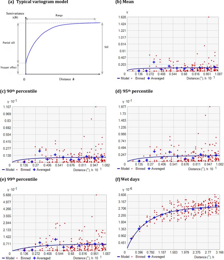
2236                                                    A. Agarwal et al.: Optimal design of hydrometric station networks

of funds for hydrometric monitoring has led to a slow but        analysis (Donges et al., 2015). EOFs, CPs, and related meth-
steady teardown of hydrometric stations over the last few        ods rely on dimensionality reduction, whereas the complex
decades globally, increasing the need for cost-effective de-     network approach allows for the study of the full complexity
sign (Mishra and Coulibaly, 2009). For example, Putthivid-       and different aspects of the statistical interdependence struc-
hya and Tanaka (2012) made an effort to design an optimal        ture and are not limited to linear and spatial-proximity con-
rain gauge network based on station redundancy and the ho-       nections. Moreover, higher-order complex network measures
mogeneity of the rainfall distribution. Adhikary et al. (2015)   (betweenness centrality, closeness centrality, and the partici-
proposed a kriging-based geostatistical approach for opti-       pation coefficient) provide additional information on the hid-
mizing rainfall networks, and Chacon-Hurtado et al. (2017)       den structure of statistical interrelationships in climatological
provided a generalized procedure for optimal rainfall and        data (Donges et al., 2015).
streamflow monitoring in the context of rainfall–runoff mod-        In this study, we propose a complex network-based
eling. Yeh et al. (2017) optimized a rain gauge network,         method to identify the influential and expendable stations
applying the entropy method on radar datasets. Most of           in a rainfall network. Several methods in the field of com-
the aforementioned studies inherently assume that expand-        plex networks have been proposed to evaluate the impor-
ing the gauge network with supplementary stations provides       tance of nodes (Chen et al., 2012; Hou et al., 2012; Jensen
more information that ultimately leads to less uncertainty       et al., 2016; Kitsak et al., 2010; Zhang et al., 2013); how-
(Wadoux et al., 2017). However, increasing the number of         ever, the application and interpretation of complex networks
stations does not necessarily decrease uncertainty (Stosic et    in hydrology (or meteorological observations) is in its in-
al., 2017). There may be expendable (not very significant)       fancy. Degree (k), betweenness centrality (B), and closeness
stations that contribute little to no information which have     centrality (CC) are measures commonly used in complex net-
the same maintenance cost as influential (highly significant)    works (Gao et al., 2013). Studies in different disciplines have
stations (Mishra and Coulibaly, 2009).                           shown that degree and betweenness centrality often outper-
   This study aims to discriminate between influential and       form other node-ranking measures (Gao et al., 2013; Liu
expendable stations in hydrometric station networks based        et al., 2016). We propose a novel measure, the weighted
on their relative information content. We propose complex        degree–betweenness (WDB), which combines k and B, to
networks as a suitable tool for this optimization problem. A     identify the stations providing the largest information to the
complex network is defined as a collection of nodes, such as     network. Our main objective is to develop a node-ranking
rain gauge stations, interconnected with links, where a link     method using complex network theory that can be used to
represents statistical similarity of the connected rain gauge    identify not only the influential but also the expendable sta-
stations. Complex networks are powerful tools in extracting      tions in large hydrometric station networks. Our study is a
information from large high-dimensional datasets (Donges         first effort to explore the benefits of complex networks in hy-
et al., 2009; Kurths et al., 2019). This nonparametric method    drology, and we acknowledge that further studies are neces-
allows for the investigation of the topology of local and non-   sary before the methodology can be considered a trustworthy
local statistical interrelationships. An example of nonlocal     optimization tool for measurement networks. Our aim is not
connections in a climate network, i.e., a complex network us-    to question the credibility of operating stations but, instead,
ing climate variables, is the global influence of the El Niño–   to propose an alternative evaluation procedure towards opti-
Southern Oscillation (ENSO) on regional rainfall (Agarwal,       mal design and redesign of observational hydrometric moni-
2019; Ferster et al., 2018) and the impact of the Atlantic       toring networks based on complex networks.
Meridional Overturning Circulation (AMOC) on air surface
temperature (Agarwal et al., 2019) via teleconnections and
ocean circulation, respectively. Once the spatial network of     2     Basics of complex networks
stations has been constructed, statistical network measures
(e.g., degree and betweenness centrality) are used to quantify   2.1    Network construction
the behavior of the network and its components for a range of
applications. Examples are the identification of the commu-      A network or a graph is a collection of entities (nodes
nity structure of stations or homogeneous regions to unravel     and vertices) interconnected with lines (links and edges), as
dominant climate modes (Agarwal et al., 2018a; Halverson         shown in Fig. 1. These entities could be anything, such as
and Fleming, 2015), catchment classification indicating hy-      humans defining a social network (Arenas et al., 2008), com-
drologic similarity (Fang et al., 2017), short- and long-range   puters constructing a web network (Zlatić et al., 2006), neu-
spatial connections in rainfall (Agarwal et al., 2018a; Boers    rons forming brain networks (Bullmore and Sporns, 2012),
et al., 2014; Jha et al., 2015), and spatiotemporal hydro-       streamflow stations creating a hydrological network (Halver-
logic patterns (Halverson and Fleming, 2015; Konapala and        son and Fleming, 2015), or climate stations describing a cli-
Mishra, 2017). Complex network analysis complements clas-        mate network (Agarwal et al., 2018b). Formally, a network
sical eigen techniques, such as empirical orthogonal func-       or graph is defined as an ordered pair Z = {N, E}; contain-
tions (EOFs) or coupled patterns (CP) maximum covariance         ing a set N = {N1 , N2 , . . .NN } of nodes and a set E of links

Hydrol. Earth Syst. Sci., 24, 2235–2251, 2020                                  www.hydrol-earth-syst-sci.net/24/2235/2020/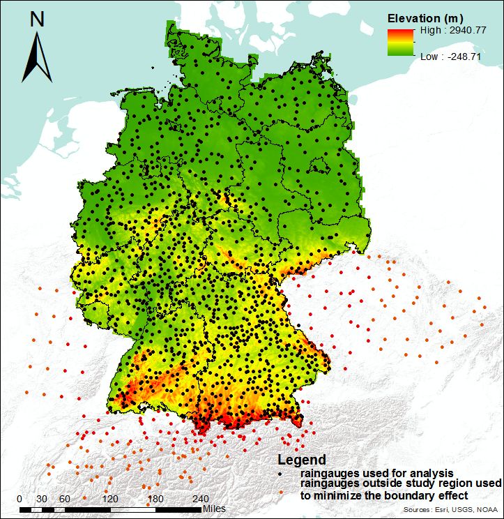
A. Agarwal et al.: Optimal design of hydrometric station networks 2237
to study heavy precipitation. Events then occur at times tlx
y
and tm , where l = 1, 2, 3, 4. . .Sx , and m = 1, 2, 3, 4. . .. . .Sy .
Events in x(t) and y(t) are considered to coincide if they
xy
occur within a time lag ±τlm , which is defined as follows:
xy x y y y y
τlm = min tl+1 − tlx , tlx − tl−1
x
, tm+1 − tm , tm − tm−1 }/2 , (2)
where Sx and Sy are the total number of such events (greater
than threshold α) that occurred in the signal x (t) and y (t),
respectively. The above definition of the time lag helps to
Figure 1. Topology of two sample networks to explain network separate independent events, which, in turn, allows one to
structures and measures. (a) Network N1 with four nodes and three
consider the fact that different processes may be responsible
links; (b) network N2 with four nodes and six links.
for the generation of events. We need to count the number of
times an event occurs in the signal x (t) after it appears in the
{i, j }, which are two-element subsets of N . In this work, we signal y (t), and vice versa, and this is achieved by defining
consider undirected and unweighted simple networks, where the quantities C (x|y) and C (y|x), where
only one link can exist between a pair of vertices, and self- Sy
Sx X
loops of the type {i, i} are not allowed. This type of net- X
C (x|y) = Jxy (3)
work can be represented by the symmetric adjacency matrix
l=1 m=1
(Eq. 1):
and
0 {i, j } 6 ∈ E
Ai,j = (1) y xy
if 0 < tlx − tm < τlm
1 {i, j } ∈ E, 1
1 y
Jxy = 2 if tlx = tm (4)
where Ai,j = 1 denotes a link between the ith and j th station,
0 else,
and 0 denotes otherwise. The adjacency matrix represents
the connections in the network. Figure 1 is a simple repre- This definition of Jxy prevents counting a synchronized
sentation of such a network, i.e., one with a set of identical event twice. When two synchronized events match exactly
y
nodes (Ni , where i = 1 to 4) connected by identical links. In (tlx = tm ), we use a factor of 1/2, as they are counted in both
general, (large) networks of real-world entities with irregular C(x|y) and C(y|x). Similarly, we can define C (y|x), and
topology are called complex networks. The links represent a from these quantities we obtain
similar evolution or variability at different nodes and can be
identified from data using a similarity measure such as the C (x|y) + C (y|x)
Qxy = q , (5)
Pearson correlation (Ekhtiari et al., 2019), synchronization (Sx − 2) Sy − 2
(Agarwal et al., 2017; Boers et al., 2019; Conticello et al.,
2018), or mutual information (Paluš, 2018). where Qxy is a normalized measure of the strength of event
synchronization between signal x (t) and y (t). This im-
2.2 Event synchronization plies Qxy = 1 for perfect synchronization and Qxy = 0 if no
events are synchronized. After repeating this procedure for
Event synchronization (ES) has been specifically designed
all pairs (x 6 = y) of stations, we obtain a similarity matrix.
to calculate nonlinear correlations among bivariate time se-
In this case, the similarity matrix for precipitation data is a
ries with events defined on them (Quiroga et al., 2002). This
square, symmetric matrix, which represents the strength of
method has advantages over other time-delayed correlation
synchronization of the extreme rainfall events between each
techniques (e.g., Pearson lag correlation), as it allows us to
pair of stations.
investigate extreme event series (such as non-Gaussian and
event-like datasets) and uses a dynamic time delay (Ozturk et 2.3 Node-ranking measures
al., 2018). The latter refers to a time delay that is adjusted ac-
cording to the two time series being compared, which allows A large number of measures have been defined to charac-
for better adaptability to the variable and region of interest. terize the behavior of complex networks. We focus here on
Various extensions for ES have been proposed, addressing, the traditional and contemporary network measures that have
for instance, boundary effects (Rheinwalt et al., 2016) and been proposed to quantify the importance of nodes in a net-
bias by varying event rates. work: degree, k; betweenness centrality, B (Agarwal et al.,
In the following, we define events by applying an α per- 2018a); “bridgeness”, Bri (Jensen et al., 2016); and degree
centile threshold at the signals x(t) and y(t). The α percentile and influence of line, DIL (Liu et al., 2016).
threshold is selected to trade off between a sufficient number
of rainfall events at each location and a rather high threshold
www.hydrol-earth-syst-sci.net/24/2235/2020/ Hydrol. Earth Syst. Sci., 24, 2235–2251, 20202238 A. Agarwal et al.: Optimal design of hydrometric station networks
2.3.1 Traditional network measures node i, NG (i). Mathematically, it is represented as
N
The degree (k) of a node in a network counts the number of
X σi (j, k)
Brii = (8)
connections linked to the node directly. The degree of any i j 6∈NG (i)∨k6∈NG (i)
σ (j, k)
node is calculated as
The neighborhood of node i(NG (i)) consists of all of the
N
X direct neighbors of node i. For example, in the networks N1
ki = Ai,j , (6) and N2, all nodes (except node 3 in N1) have B = 0; hence,
j =1 Bri = 0. However, node 3 in network N1 has all of the nodes
in the direct neighborhood; hence, it also has Bri = 0.
where N is the total number of nodes in a network. For exam- The degree and influence of line (DIL), introduced by Liu
ple, the degree of nodes 1, 2, and 4 in network N1 (Fig. 1a) et al. (2016), considers the node degree (k) and the impor-
is 1, and for node 3 it is 3. In network N2 (Fig. 1b), all tance of line (I ) to rank the nodes in a network:
nodes have degree 3. The degree can explain the importance X ki − 1
of nodes to some extent, but nodes that have the same de- DILi = ki + Ieij · , (9)
gree may not play the same role in a network. For instance, j =N (i)
ki + kj − 2
G
a bridging node connecting two important nodes might be
where the line between node i and j is eij , and its importance
very relevant, although its degree could be much lower than
is defined as Ieij = Uλ , where U = (ki − p − 1) · (kj − p − 1)
the value of less important nodes.
reflects the connectivity ability of a line (link), p is the num-
The betweenness centrality (B) is a measure of the con-
ber of triangles with one edge eij , and λ = p2 +1 is defined as
trol that a particular node exerts over the interaction between
an alternative index of line eij . NG (i)) is the set of neighbors
the remaining nodes. In simple words, B describes the abil-
of node i (for detailed explanation see Liu et al., 2016). The
ity of nodes to control the information flow in networks. To
equation for DIL suggests that all the nodes with ki = 1 will
calculate betweenness centrality, we consider every pair of
have DILi = 1, as the second term of the equation will be
nodes and count how many times a third node can interrupt
zero. Hence, in network N1, all nodes, except node 3, have
the shortest paths between the selected node pair. Mathemat-
DIL = 1. Node 3 has DIL = 3 equal to its degree, as the sec-
ically, the betweenness centrality (B) of any i node is
ond term is zero (all of the connected nodes 1, 2, and 4 have
N
kj = 1; hence, Ieij = 0). All of the nodes in network N2 have
X σi (j, k) DIL = 3.
Bi = , (7)
i6=j 6=v∈{V }
σ (j, k)
3 Methodology
where σ (j, k) represents the number of links along the short-
est path between node j and k, and σi (j, k) is the number of We will first propose a new node-ranking measure that we
links of the shortest path running through node i. In network call weighted degree–betweenness (WDB). We will then
N1 (Fig. 1a), B of node 3 is 3, i.e., node 3 can disturb the compare the efficacy of this measure with the existing tra-
information transfer between all of the three pairs 1–2, 1–4, ditional and contemporary node-ranking methods using two
and 2–4, and for other nodes B = 0. In network N2 (Fig. 1b), synthetic networks.
all nodes have B = 0 because no node can interrupt the in-
formation flow. Thus, node 3 is a critical node in network N1 3.1 Weighted degree–betweenness
but not in the network N2.
WDB is a combination of two network measures, degree and
2.3.2 Contemporary network measures betweenness centrality. We define the WDB of a particular
node i as the sum of the betweenness centrality of node i and
Jensen et al. (2016) developed the bridgeness measure, Bri, all directly connected nodes j, j = 1, 2, 3. . .ki in proportion
to distinguish local centers, i.e., nodes that are highly con- to their contribution to node i. The WDB of a node i is given
nected to a part of the network (e.g., highly correlated sta- by
tions in a homogeneous region), from global bridges, i.e.,
WDBi = Bi + Ii , (10)
nodes that connect different parts of a network (Fig. 2; e.g.,
teleconnection between Indian rainfall and climate indices). where Bi is the betweenness centrality of node i, and Ii
Bri is a decomposition of the betweenness centrality (B) stands for the cumulative effect of the influence or con-
into a local and a global contribution. Therefore, the Bri value tribution of the directly connected nodes of i, which are
of node i is always smaller than or equal to the correspond- j = 1, 2, 3, . . ., ki , calculated as follows:
ing B value, and they only differ by the local contribution ki
of the first direct neighbors. To calculate Bri, we consider
X Bj · (kj − 1)
Ii = , (11)
the shortest path between nodes outside the neighborhood of (k + kj − 2)
j =1 i
Hydrol. Earth Syst. Sci., 24, 2235–2251, 2020 www.hydrol-earth-syst-sci.net/24/2235/2020/A. Agarwal et al.: Optimal design of hydrometric station networks 2239
where ki is the degree of node i, and kj is the degree of the reflects its role as a global bridge node. WDB distinguishes
nodes j which are directly connected to node i. between nodes 1, 2, and 3 (WDB = 14.4) and between nodes
7 and 8 (WDB = 13.3), which is important in case we need
3.2 Comparison with existing node-ranking measures to sequentially rank nodes.
using synthetic networks We further evaluate WDB using the network measures Bri.
For this comparison, we use the same synthetic network as
In this section, we motivate the development of the new Jensen et al. (2016), which is shown in Fig. 3. Betweenness
node-ranking measure, WDB, by comparing it to existing centrality once again assigns a smaller value to the global
measures. Identifying nodes that occupy interesting posi- bridge (node 6) than to the local centers (nodes 4 and 7).
tions in a real-world network using node ranking helps to Bridgeness expresses the higher importance of node 6 com-
extract meaningful information from large datasets at little pared with nodes 4 and 7; however, it does not distinguish
cost. Usually, the measures of degree (ki ) and betweenness between all of the other nodes in the network (nodes 1, 2,
centrality (Bi ) are common node-ranking metrics (Gao et 3 . . . have Bri = 0). Similarly, DIL misses representing the
al., 2013; Okamoto et al., 2008; Saxena et al., 2016). The bridge nodes by assigning higher values to local centers.
network measures ki , Bi and WDBi of each node are given WDB ranks the nodes, preferably following their role in the
for an undirected and unweighted network Z = (N, E) with network as global bridges, local centers, and end nodes. For
8 nodes and 11 edges, shown in Fig. 2 along with the node example, WDB is also able to differentiate between nodes
number. 4 and 7 for which the bridgeness measure provides equal
In general, high-degree nodes represent most connected scores.
(highly correlated) nodes in a network. Rheinwalt et
al. (2015) considered these highly correlated nodes of a ho- 3.3 Evaluation of the proposed measure for a rain
mogeneous precipitation community as local centers repre- gauge network
senting homogenous precipitation patterns for that particular
community. Agarwal et al. (2018a) defined local centers as In the context of hydrometric station networks, we hypoth-
the nodes with maximum intra-community links and min- esize that higher ranking nodes are more influential stations
imum intercommunity links based on the Z–P space ap- in the complex network and also in the observation network.
proach. However, degree alone cannot distinguish the roles Losing such stations could reduce the network stability and
of nodes in the sample network as seen for nodes 5, 7, and 8, efficiency given their role in bridging different communities
which have the same degree (ki = 2), although node 5 serves (processes) and capturing detailed process information com-
as a bridge node linking the two parts of the network. In pared with lower ranking stations. Stations with the lowest
a larger complex network, such bridge nodes have strate- ranks in the network are the least influential and are seen
gic relevance as most of the information can be accessed as expendable stations. For example, a bridging node would
quickly just by capturing these nodes. For example, Kurths be located between two regions of different variability and,
et al. (2019) quantified the spatial diversity of Indian rainfall therefore, plays an important role in estimating the spatial
teleconnections at different timescales by identifying link- border between these regions. A low-ranked node would
ages between climatic indices (e.g., El Niño–Southern Os- be located within a (more or less) homogenous region and
cillation, Indian Ocean Dipole, North Atlantic Oscillation, would not provide additional knowledge about the spatial
Pacific Decadal Oscillation, and Atlantic Multidecadal Os- variability. To test this hypothesis, we apply the proposed
cillation) and seven Indian rainfall stations (bridge nodes). node-ranking measure to a hydrometric station network, con-
Betweenness centrality has a higher power with respect sisting of more than 1000 stations in Germany. The benefit
to significantly discriminating between different roles com- of WDB is that it can capture the bridge nodes in the hydro-
pared with ki . For example, nodes 4 and 5 have the highest Bi metric station network that are adequate to quantify the lo-
(B4 = B5 = 24) followed by node 6 (B6 = 20). Conversely, cal and nonlocal rainfall variability for process identification,
Bi gives equal scores to local centers (node 4), i.e., nodes for interpolation of measurements, and for transferability of
of high ki to a single region, and to global bridges (node precipitation measurements across locations. In contrast, ex-
5), which connect detached regions. As mentioned, global pandable stations correspond to sites of spatially extended
bridges connect different parts of a network (e.g., teleconnec- coherent rainfall that surround a local center which repre-
tion between Indian rainfall and ENSO). Measuring and in- sents the variability of such regions. Stations within such re-
terpretation of large spatial variability, process identification, gions of coherent rainfall provide redundant information and
interpolation of measurements, and transferability of precip- can be removed (except the local center) without loss of in-
itation measurements across locations, would be limited in formation. The information loss caused by removing stations
the absence of high-Bi nodes. is quantified by two measures: (a) the decline rate of network
The proposed measure – WDB – has higher discrimination efficiency, and (b) the relative kriging error.
power than betweenness centrality. Node 5 has the highest
WDB score and is ranked as the most influential node, which
www.hydrol-earth-syst-sci.net/24/2235/2020/ Hydrol. Earth Syst. Sci., 24, 2235–2251, 20202240 A. Agarwal et al.: Optimal design of hydrometric station networks
Figure 2. The synthetic network to explain the degree (k), betweenness centrality (B), and weighted degree–betweenness (WDB) measures,
showing the node number (1 to 8) followed by the degree, betweenness centrality value, and WDB values in brackets [k, B, WDB]. The
degree and betweenness are limited with respect to distinguishing the role of different nodes in the network and centers from bridges,
respectively.
Figure 3. The synthetic network used to compare the network measures, betweenness centrality, bridgeness, and DIL, with the proposed
measure, WDB. Numbers 1 to 11 are node counts, and values in brackets represent the network measure values in the following order: [B,
Bri, DIL, and WDB]. Node 6 is a global bridge node that connects two subnetworks. Nodes 4 and 7 are hubs that are connected to most of
the nodes in the subnetworks. Nodes 5, 10, and 11 are the dead-end nodes.
3.3.1 Decline rate of network efficiency rate of network efficiency µ is defined as
The decline rate of network efficiency quantifies the decrease ηnew
µ = 1− , (13)
in information flows within a network when nodes are re- ηold
moved as
where ηnew is the efficiency of the network after removing
1 X nodes, and ηold is the efficiency of the complete network.
η= ηij , (12) We hypothesize that the network efficiency decreases
N (N − 1) n 6=n
i j more strongly when higher ranking stations are removed, i.e.,
bridge nodes.
where N is the total number of nodes in a network, and ηij
is the efficiency between nodes ni and nj . ηij is inversely 3.3.2 Relative kriging error
related to the shortest path length: ηij = 1/dij , where dij is
the shortest path between nodes ni and nj . The average path As second measure to evaluate the information loss when sta-
length L measures the average number of links along the tions are removed from the network, we use a kriging-based
shortest paths between all possible pairs of network nodes. A geostatistical approach (Adhikary et al., 2015; Keum et al.,
network with small L is highly efficient, because two nodes 2017). Kriging is an optimal surface interpolation technique
are likely to be separated by only a few links. The decline that assumes that the distance or direction between a sample
Hydrol. Earth Syst. Sci., 24, 2235–2251, 2020 www.hydrol-earth-syst-sci.net/24/2235/2020/A. Agarwal et al.: Optimal design of hydrometric station networks 2241
of observations reflects a spatial correlation that can be used
to explain variation in the surface. (Adhikary et al., 2015).
The algorithm estimates unknown variable values at unsam-
pled locations in space, where no measurements are avail-
able, based on the known sampling values from the surround-
ing areas (Hohn, 1991; Webster and Oliver, 2007). Ordinary
kriging is used in this study to interpolate rainfall data and
estimate the kriging error. The kriging estimator is expressed
as
n
X
Z ∗ (xo ) = wi Z(xi ), (14)
i=1
where Z ∗ (xo ) refers to the estimated value of Z at the de-
sired location xo , wi represents weights associated with the
observation at location xi with respect to xo , and n indicates
the number of observations within the domain of the search
neighborhood of xo for performing the estimation of Z ∗ (xo ).
Ordinary kriging is implemented using ArcGISv10.4.1 (Red-
lands, CA, USA) and its geostatistical analyst extension
(Johnston et al., 2001).
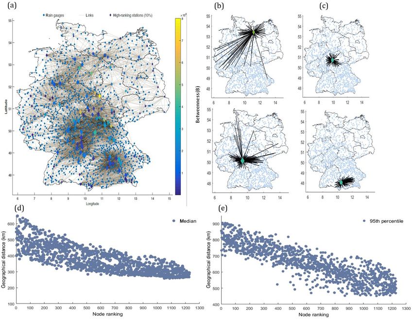
The kriging variance σz2 (xo )in the ordinary kriging can be Figure 4. Location of rain stations in Germany and adjacent areas.
computed as (Adhikary et al., 2015; Xu et al., 2018) Black dots indicate stations lying inside Germany that are used in
n n the analysis. Red dots indicate stations outside of Germany that are
X X
σz2 = µz + wi γ (hoi ) with wi = 1, used for network construction only in order to minimize the bound-
i=1 i=1
ary effect. © Esri, USGS, NOAA.
where γ (h) is the variogram value for the distance h, hoi is
the distance between observed data points xi and xj , µz is 4 Application to an extensive rain gauge network
the Lagrangian multiplier in the Z scale, h0j is the distance
between the unsampled location x0 (where the estimation is 4.1 Rainfall data
desired) and sample locations xi , and n is the number of sam-
To evaluate the proposed measure in the context of the op-
ple locations.
timal design of hydrometric networks, we apply it to an ex-
The square root of the kriging variance, also known as
tensive network of rain stations in Germany and adjacent ar-
the kriging standard error (KSE), is used as a gauge net-
eas (Fig. 4). The data covers 110 years at a daily resolution
work evaluation factor. We estimate the increase in the krig-
(1 January 1901 to 31 December 2010). The 1229 rain sta-
ing standard error across the study area when stations are
tions in Germany (blue dots in Fig. 4) are operated by the
removed to evaluate the performance of the WDB measure
German Weather Service. Data processing and quality con-
in identifying influential and expendable stations in a large
trol were performed according to Österle et al. (2006), and,
network.
in this study, we assume that data are free of measurement
The relative kriging error before and after removing the
errors. A total of 211 stations from different sources outside
stations is denoted as
Germany (red dots in Fig. 4) were included in the analysis to
KSEnew − KSEold minimize spatial boundary effects in the network construc-
R (%) = × 100, (15)
KSEold tion; however, these stations were excluded from the node-
ranking analysis. For parts of France, precipitation data on a
where KSEnew denotes the standard kriging error after re- 0.22◦ ×0.22◦ rotated pole grid from E-OBS were used (Hay-
moving stations, and KSEold is the error for the original net- lock et al., 2008).
work. We hypothesize that the increase in the relative krig-
ing error is higher when removing high-ranking stations. To 4.2 Network construction
cover a broad range of rainfall characteristics, the error is cal-
culated for different statistics, i.e., the mean, 90th, 95th, and We begin the network construction by extracting event time
99th percentile rainfall, and the number of wet days (precip- series from the 1229 daily rainfall time series. The event se-
itation greater than 2.5 mm). ries represent heavy rainfall events, i.e., precipitation exceed-
ing the α = 95th percentile at that station (Rheinwalt et al.,
2016). The 95th percentile is a trade-off between having a
www.hydrol-earth-syst-sci.net/24/2235/2020/ Hydrol. Earth Syst. Sci., 24, 2235–2251, 20202242 A. Agarwal et al.: Optimal design of hydrometric station networks
sufficient number of rainfall events at each location and a
rather high threshold to study heavy precipitation. All rain-
fall event series are compared with each other using event
synchronization (Sect. 2.2), which is the base for deriving
a complex network. This results in the similarity matrix Q,
where the entry at index pair (i, j ) defines synchronization
in the occurrence of heavy rainfall events at station i and sta-
tion j (Eq. 5).
Applying a certain threshold (θ ) to the Q matrix yields
Q
the adjacency matrix (Eq. 1). Here, θxy is a chosen thresh-
old, Aij = 1 denotes a link between the ith and j th sites,
and Aij = 0 denotes otherwise. The adjacency matrix repre-
sents a rain gauge network, and complex network theory can Figure 5. Decline rate of network efficiency corresponding to the
subsequently be employed to reveal properties of the given removal of each node in the rainfall network. In each implemen-
network. tation, only one node is removed from the network according to
ranking with replacement (bootstrapping).
Two criteria have been proposed to generate an adjacency
matrix from a similarity matrix, such as the fixed amount of
link density (Agarwal et al., 2018b, 2019) or global fixed rank). After n = 1229 (number of nodes) trials, we investi-
thresholds (Jha et al., 2015; Sivakumar and Woldemeskel, gate the relationship between µ and the node ranking mea-
2014). However, both criteria are subjective and may lead sured by WDB. We expect an inverse relationship between
to the presence of weak and nonsignificant links in the com- µ and WDB: the higher the node ranking, the more impor-
plex network. These nonsignificant links might obscure the tant the node, leading to a higher loss in network efficiency
topology of strong and significant connections. To minimize (Fig. 5). µ is high for high-ranking stations and decays with
Q
these threshold effects, we choose the threshold θi,j objec- node ranking. Interestingly, µ < 0 for very low-ranking sta-
tively by considering all links in the network that are sig- tions, i.e., the network efficiency increases when single, low-
nificant. A link is significant (i.e., two stations are signifi- ranking stations are removed. This is explained by the de-
cantly synchronized) if the synchronization value exceeds the crease in the redundancy in the network when such stations
Q
θi,j = 95th percentile (corresponding to a 5 % significance are removed.
level) of the synchronization obtained by two synthetic vari- Secondly, we successively remove a larger number of sta-
ables that have the same number of events but are distributed tions, from 1 to 123 stations (10 %), considering three cases.
randomly in the time series (i.e., both event series are inde- In case I, we remove up to 10 % of the highest ranking sta-
pendent). We calculate ES for 100 pairs of such random time tions. This implies that in the first iteration, we remove the
series and derive the 95th percentile of the resulting ES distri- top-ranked station; in the second iteration, we remove the top
bution. Using this 5 % significance level, we assume that syn- two stations; and so on. Figure 6 shows an apparent increase
chronization cannot be explained by chance if the ES value in µ as more and more influential stations are removed. In
between two stations is larger than the 95th percentile of the case II, up to 10 % of the lowest ranking stations are suc-
test distribution. Here, we select the 5 % significance level, cessively removed. The efficiency increases when the lowest
as it is generally a well-accepted criterion in statistics. To ranking stations are removed. In case III, up to 10 % of sta-
validate the results, we repeated the analysis for the 90–99th tions are randomly removed. Case III is repeated 10 times in
percentile threshold range and observed that the node rank- order to understand the effect of random sampling. In gen-
ing is robust against the threshold selection. For the sake of eral, µ increases with the removal of random stations. How-
brevity, detailed results are presented for the 95th percentile ever, the effect is much lower (in absolute terms) than the ef-
threshold only. fect of removing the respective high- or low-ranking stations.
The variation in µ between the 10 trials and within 1 trial is
4.3 Decline rate of network efficiency caused by randomness. For example, µ rises instantaneously
when the algorithm picks up a high-ranking station.
In this section, we evaluate the ranking of stations derived
from the proposed WDB measure using the decline rate of 4.4 Relative kriging error (R)
network efficiency. The rain gauges are ranked in decreas-
ing order according to their WDB values. Highly ranked rain As the second approach to assess the suitability of the WDB
gauges are interpreted as the most influential stations, and for identifying influential and expendable stations, we ana-
low ranked gauges are interpreted as expendable stations. lyze the change in the kriging error (R) when stations are
Firstly, we analyze the decline rate of network efficiency removed from the network. We first estimate the kriging stan-
µ when one station is removed from the network. In each dard error KSEold across the study area for all 1229 stations.
trial, we remove only one station (starting with the highest We then measure the kriging standard error across the study
Hydrol. Earth Syst. Sci., 24, 2235–2251, 2020 www.hydrol-earth-syst-sci.net/24/2235/2020/A. Agarwal et al.: Optimal design of hydrometric station networks 2243
degree and betweenness centralities) and contemporary (i.e.,
bridgeness and DIL) measures by applying it to prototypi-
cal situations. The results show that degree and betweenness
centrality are unable to differentiate between different roles
of a node in a network. Although the contemporary network
measures bridgeness and DIL showed higher power with re-
spect to discriminating different roles, they do not provide
a nuanced picture of marginal differences, for example, be-
tween a local center and a global bridge. Hence, our tests
with synthetic networks suggest that the WDB is superior
with respect to distinguishing different roles, compared with
Figure 6. Decline rate of network efficiency as a function of the existing measures, and provides a unique value to each node
number of stations removed from the network. In case I, up to 10 % depending on its importance and influence in our test net-
of the highest ranking stations are removed (black); in case II, up to works.
10 % of the lowest ranking stations are removed (red); and in case Besides this methodological development, this study pro-
III, up to 10 % of randomly drawn stations are removed (10 trials; poses using WDB to support the optimal design of large hy-
blue). drometric networks. Its preliminary application to the Ger-
man rain gauge network shows its ability to rank the nodes
in such large hydrometric networks. For example, removing
area when stations are removed (Knew ) and calculate the
low-ranking stations does not have an adverse impact on net-
change in the error (Eq. 15). The variogram is kept constant
work efficiency, and kriging errors are hardly increase. This
during the network modifications. Similar to the evaluation
is explained by the redundancy in the information that these
using the decline rate of network efficiency in Sect. 4.3, three
stations provide, which, in turn, is attributed to the similarity
cases are investigated: removing 10 % of the highest ranking
between the gauges due to common driving mechanisms or
stations, removing 10 % of the lowest ranking stations, and
spatial similarity, as advocated by Tobler’s law of geography
10 trials removing 10 % of the stations randomly.
(Tobler, 1970). Our analysis suggests that the WDB identi-
The change in the kriging error is calculated for five char-
fies the expendable nodes correctly, as shown by the decline
acteristics, i.e., mean, 90 %, 95 %, and 99 % percentile, and
rate of efficiency and the insignificant change in the relative
the number of wet days (Table 1). For each case and rainfall
kriging error. Conversely, WDB awards stations that provide
characteristic, we run the model 100 times; the mean value
unique information as it considers different aspects of the
of R is reported in Table 1.
spatiotemporal relationships in the observation network.
Removing 10 % of the high-ranking stations (case I) leads
We further analyze the characteristics of the stations with
to positive and high (between 12 % and 73 %) relative krig-
the highest ranks. We plot the network (Fig. 7a) correspond-
ing errors for all five statistics considered, i.e., the kriging er-
ing to 10 % (∼ 122) of the highest ranking stations, i.e.,
ror increases substantially when these stations are removed.
all the links originating from these 122 stations alone. The
In contrast, when 10 % of the lowest ranking stations (case
size and color of each diamond-shaped rain gauge mark
II) are not considered, the R values are small. The relative
shows their degree and betweenness centrality, respectively.
errors in estimating the mean, percentile rainfall characteris-
All other stations are plotted in the background without
tics (90th and 95th), and the number of wet days at ungauged
highlighting their degree and betweenness. We further plot
locations is lower than 5 %, suggesting that these stations do
the connections corresponding to two high-ranking stations
not contribute much information. In case III, i.e., removing
(Fig. 7b) and two low-ranking stations (Fig. 7c) to ease in-
stations randomly, rather high errors are observed (between
terpretation. Although the degree of these four stations is
5 % and 51 %); however, they are much smaller than in case
roughly the same, the connections of low-ranking stations
I.
are regionally confined, and they rather reflect the similar-
ity in rainfall variability within (homogenous) regions. The
5 Discussion highest ranked stations are not governed by local or global
features alone but rather by a combination of both (Fig. 7a).
Building on the young science of complex networks, a novel This observation could reflect the critical nodes in pathways
node-ranking measure – the weighted degree–betweenness, of atmospheric moisture transport, extreme rainfall propaga-
WDB – is proposed. The proposed method, which is based tion, or, in case of high betweenness centrality, it could in-
on degree and betweenness centrality, does not only account dicate a handful of stations that are positioned between the
for the local (captured by degree) and global (captured by large communities and, unlike most stations, tend to possess
betweenness centrality) characteristics of nodes but also for intercommunity connections (Halverson and Fleming, 2015;
the cumulative contribution of the directly connected (local- Molkenthin et al., 2015; Tupikina et al., 2016). We plot the
ized) nodes. We compared WDB with other traditional (i.e., median (Fig. 7d) and 95th percentile (Fig. 7e) of the geo-
www.hydrol-earth-syst-sci.net/24/2235/2020/ Hydrol. Earth Syst. Sci., 24, 2235–2251, 20202244 A. Agarwal et al.: Optimal design of hydrometric station networks
Table 1. Relative kriging error for the three different cases. The relative kriging error for case III is the average across 10 trials. An asterisk
indicates a high relative error greater than 5 %.
Case Removal of stations Relative kriging error R (%)
Mean 90th percentile 95th percentile 99th percentile Wet days
I 10 % highest ranking 11.7∗ 29.9∗ 73.3∗ 58.1∗ 62.1∗
II 10 % lowest ranking 0.09 4.2 3.7 8.1∗ 2.9
III 10 % randomly selected 6.4∗ 23.3∗ 51.3∗ 46.6∗ 4.7
Figure 7. (a) Connections and location of 10 % (∼ 122) of the highest ranking rain gauges. The size and color of the diamond markers
indicate the degree and betweenness centrality of the rain gauges, respectively. Connections corresponding to (b) two high-ranking stations
(station IDs 21 320 and 16149) and (c) two low-ranking stations (station IDs 26132 and 20356). (d) The median and (e) 95th percentile
geographical distance plotted against node ranking.
graphical distance between all of the connected rain gauges plicitly affirming that the WDB measure has the potential to
to test whether the long-range connections of the selected capture highly influential nodes in the network.
nodes in Fig. 7b are a typical feature of highly ranked sta- The results presented in Fig. 7 support the conclusion de-
tions. There is a clear association between rank and distance: rived from the kriging error analysis in Sect. 4.4. Remov-
highly ranked stations tend to show longer connections, im- ing an influential station (Fig. 7b) fosters higher kriging er-
rors than removing a random low-ranking station (Fig. 7c).
Hydrol. Earth Syst. Sci., 24, 2235–2251, 2020 www.hydrol-earth-syst-sci.net/24/2235/2020/A. Agarwal et al.: Optimal design of hydrometric station networks 2245 Hence, the new measure could support the optimal design of large hydrometric networks or the redesign of existing hy- drometric networks by ranking nodes. The influence of the similarity measure, the number of stations present in the net- work, the spatial boundary, data length, and threshold has to be further investigated before the method can become fully operational. Acknowledging the infant state of complex net- work science in hydrology, we emphasize the need for more intensive application, new interpretable network measures, and visualization tools to find the modern solutions of tradi- tional hydrological problems. 6 Conclusions This study proposes the application of complex networks to the optimization of hydrometric monitoring networks. In ad- dition, it proposes a novel node-ranking measure for identify- ing influential and expendable nodes in a complex network. The new network measure, weighted degree–betweenness (WDB), combines the measures of degree and betweenness centralities. It does not only account for the local and global characteristics of nodes but also the cumulative contribution of the directly connected (localized) nodes. Its comparison to existing measures demonstrates that WDB is more sensi- tive to the different roles of nodes, such as global connecting nodes or local centers, as it considers various aspects of the spatiotemporal relationships in observation network. We propose using WDB for ranking rain gauges in hydro- metric networks. Applying WDB to a network of 1229 rain gauges in Germany allows for the identification of influen- tial and expendable stations. Two criteria, the decline rate of network efficiency and the kriging error, are used to evalu- ate the performance of the proposed node-ranking measure. The results suggest that the proposed measure is indeed ca- pable of effectively ranking the stations in large hydrometric networks. We suggest that the proposed measure is not only useful for rain gauge networks but also has the potential to support the selection of an optimal number of stations for prediction in ungauged basins (PUBs) and the estimation of missing val- ues by identifying influential stations in the region. Similarly, the proposed method can be applied to gridded satellite data (e.g., rainfall and soil moisture) to locate the strategic points where stations should be installed to ensure a highly efficient observation network. However, acknowledging the rarity of complex network studies in hydrology and the preliminary work of our study, the advantages and disadvantages of this new measure need to be further investigated. This includes addressing threshold and spatial boundary issues of the net- work, developing new physical interpretable measures, and visualization tools. More studies are needed to prove the ben- efits of complex network science in hydrometric network de- sign. www.hydrol-earth-syst-sci.net/24/2235/2020/ Hydrol. Earth Syst. Sci., 24, 2235–2251, 2020
2246                                                          A. Agarwal et al.: Optimal design of hydrometric station networks

Appendix A: Spatially embedded network construction                          We compute the WDB score for each station using
                                                                          Eq. (10). Station 3 shows the highest WDB score (Fig. A1).
We randomly select 11 rain gauge stations in Germany to                   This station accounts for the local and global characteristics
illustrate the network construction (Sect. 2.1) from observa-             of the network, in addition to the cumulative effect of its di-
tions (Fig. A1). We first compute the cross-correlation be-               rect neighbors, i.e., stations 2, 5, 7, 8, and 10. We infer two
tween each pair of stations (Table A1) and apply the 90th                 groups (stations 1, 2, 3, 6, and 8 and stations 3, 4, 5, 7, 9,
percentile threshold (0.44), i.e., only links between stations            10, and 11) in the network that are bridged by station 3. This
with values higher than 0.44 are shown.                                   node is particularly crucial in the context of measuring pro-
                                                                          cess, process identification, or interpolation of measurements
                                                                          (Jensen et al., 2016).

Figure A1. Location of 11 randomly selected rain stations used to construct a complex network based on the cross-correlation similarity
measure and 90th percentile threshold. Diagonal values (autocorrelation) in Table 1 have been ignored in network construction. Numbers 1
to 11 are node counts, and the values in brackets represent the WDB values.

Table A1. Cross-correlation values along with the geographical location of 11 rain gauges selected for illustrative purposes.

               Nodes     Long.      Lat.      1       2       3       4       5      6       7       8       9     10      11
               1          6.55    50.42    1.00    0.46    0.50   0.32     0.33   0.59    0.41    0.42   0.27    0.32    0.24
               2          8.83    50.52    0.46    1.00    0.58   0.38     0.38   0.43    0.39    0.54   0.30    0.40    0.27
               3          9.42    50.13    0.50    0.58    1.00   0.41     0.51   0.45    0.49    0.48   0.35    0.50    0.36
               4         10.73    51.28    0.32    0.38    0.41   1.00     0.45   0.27    0.30    0.31   0.27    0.41    0.29
               5         11.57    50.12    0.33    0.38    0.51   0.45     1.00   0.30    0.41    0.33   0.40    0.64    0.46
               6          6.27    49.93    0.59    0.43    0.45   0.27     0.30   1.00    0.39    0.44   0.24    0.30    0.22
               7          8.52    48.62    0.41    0.39    0.49   0.30     0.41   0.39    1.00    0.39   0.52    0.45    0.41
               8          8.03    49.88    0.42    0.54    0.48   0.31     0.33   0.44    0.39    1.00   0.29    0.37    0.25
               9         10.33    48.68    0.27    0.30    0.35   0.27     0.40   0.24    0.52    0.29   1.00    0.46    0.51
               10         10.9    49.72    0.32    0.40    0.50   0.41     0.64   0.30    0.45    0.37   0.46    1.00    0.50
               11           12    48.97    0.24    0.27    0.36   0.29     0.46   0.22    0.41    0.25   0.51    0.50    1.00

Hydrol. Earth Syst. Sci., 24, 2235–2251, 2020                                            www.hydrol-earth-syst-sci.net/24/2235/2020/
A. Agarwal et al.: Optimal design of hydrometric station networks 2247
Appendix B: Variogram modeling The variogram models are a function of three parameters;
the range, the sill, and the nugget (Fig. B1a). The range is
The kriging modeling assumes a theoretical variogram func- the distance where the models first flatten out, i.e., station
tion that is fitted with an experimental variogram of the ob- locations within the range distance are spatially correlated,
served data. The experimental variogram (γ (h)) is calculated whereas locations farther apart are not. The value of γ at the
from the observed data as a function of the distance of sepa- range is called the sill, which is estimated by the variance of
ration (h) (Adhikary et al., 2015) and is given by the sample. The nugget represents measurement errors and/or
microscale variation at very small spatial scales and is seen
1 N(h)
Xh i
as a discontinuity at the origin of the variogram model. The
γ (h) = (Y (i) − Y (j ))2 , (B1)
2N (h) i=1 ratio of the nugget to the sill is known, as the nugget effect
and may be interpreted as the percentage of variation in the
where N (h) is the number of sample data points separated data that is not related to space. The difference between the
by the distance h; i and j represent sampling locations sepa- sill and the nugget is known as the partial sill (Adhikary et
rated by h; and Y (i) and Y (j ) indicate values of the observed al., 2015; Keum et al., 2017).
variable Y , measured at the corresponding locations i and j , The values of all parameters and the resulting variogram
respectively. The theoretical variogram function (γ ∗ (h)) al- for the daily mean, 90th, 95th, and 99th percentile precipita-
lows for the analytical estimation of variogram values for any tion, and number of wet days are reported in Table B2 and
distance and provides the unique solution for weights with Fig. B1b–d, respectively. The variogram was kept constant
intermediate steps required for kriging interpolation (Ad- during network reductions.
hikary et al., 2015).
Table B1. Parameter values for the fitted variogram.
Parameters Mean 90th percentile 95th percentile 99th percentile Wet days
Nugget 0.0056 0 0 0 0.805
Range 0.0781 0.0782 0.0782 0.0782 2.361
Partial sill 0.102 1.055 2.140 6.808 2.761
www.hydrol-earth-syst-sci.net/24/2235/2020/ Hydrol. Earth Syst. Sci., 24, 2235–2251, 20202248 A. Agarwal et al.: Optimal design of hydrometric station networks Figure B1. Typical variogram model (a) and fitted variogram models for the daily mean (b), 90th (c), 95th (d), and 99th (e) percentile precipitation, and number of wet days (f). Hydrol. Earth Syst. Sci., 24, 2235–2251, 2020 www.hydrol-earth-syst-sci.net/24/2235/2020/
A. Agarwal et al.: Optimal design of hydrometric station networks                                                                       2249

Data availability. The authors used Germany’s precipitation data         Agarwal, A.: Unraveling spatio-temporal climatic patterns via
which are maintain and provided by German Weather Service. The             multi-scale complex networks, Universität Potsdam, Potsdam,
data are publicly accessible at https://opendata.dwd.de/ (last access:     2019.
30 January 2018). Further preprocessing of the data was carried out      Agarwal, A., Marwan, N., Rathinasamy, M., Merz, B., and Kurths,
by Potsdam Institute of climate impact research (see Oesterle, 2001;       J.: Multi-scale event synchronization analysis for unravelling
Conradt et al., 2012).                                                     climate processes: a wavelet-based approach, Nonlin. Pro-
                                                                           cesses Geophys., 24, 599–611, https://doi.org/10.5194/npg-24-
                                                                           599-2017, 2017.
Author contributions. AA designed and implemented the research           Agarwal, A., Marwan, N., Maheswaran, R., Merz, B., and Kurths,
model. AA developed the node-ranking algorithm and performed               J.: Quantifying the roles of single stations within homogeneous
several test cases. UO tested the node-ranking algorithm on various        regions using complex network analysis, J. Hydrol., 563, 802–
other networks. NM, JK, and BM closely supervised the work and             810, https://doi.org/10.1016/j.jhydrol.2018.06.050, 2018a.
encouraged AA to investigate the node-ranking algorithm for the          Agarwal, A., Maheswaran, R., Marwan, N., Caesar, L.,
hydrological dataset. AA implemented the method and performed              and Kurths, J.: Wavelet-based multiscale similarity mea-
the analyses and tests. RM, JK, and BM helped to interpret the find-       sure for complex networks, Eur. Phys. J. B, 91, 296,
ings. All authors discussed the results and contributed to the final       https://doi.org/10.1140/epjb/e2018-90460-6, 2018b.
paper.                                                                   Agarwal, A., Caesar, L., Marwan, N., Maheswaran, R., Merz, B.,
                                                                           and Kurths, J.: Network-based identification and characterization
                                                                           of teleconnections on different scales, Sci. Rep.-UK, 9, 8808,
Competing interests. The authors declare that they have no conflict        https://doi.org/10.1038/s41598-019-45423-5, 2019.
of interest.                                                             Arenas, A., Díaz-Guilera, A., Kurths, J., Moreno, Y., and Zhou, C.:
                                                                           Synchronization in complex networks, Phys. Rep., 469, 93–153,
                                                                           https://doi.org/10.1016/j.physrep.2008.09.002, 2008.
                                                                         Boers, N., Rheinwalt, A., Bookhagen, B., Barbosa, H. M. J.,
Acknowledgements. This research was funded by the Deutsche
                                                                           Marwan, N., Marengo, J., and Kurths, J.: The South Amer-
Forschungsgemeinschaft (DFG; GRK grant no. 2043/1) within the
                                                                           ican rainfall dipole: A complex network analysis of extreme
“Natural Hazards and Risk in a Changing World” (NatRiskChange)
                                                                           events: BOERS ET AL., Geophys. Res. Lett., 41, 7397–7405,
graduate research training group at the University of Potsdam (http:
                                                                           https://doi.org/10.1002/2014GL061829, 2014.
//www.uni-potsdam.de/natriskchange, last access: 15 July 2019).
                                                                         Boers, N., Goswami, B., Rheinwalt, A., Bookhagen, B., Hoskins,
AA acknowledges the funding support provided by the Indian Insti-
                                                                           B., and Kurths, J.: Complex networks reveal global pat-
tute of Technology Roorkee through a faculty initiation grant (grant
                                                                           tern of extreme-rainfall teleconnections, Nature, 566, 373–377,
no. IITR/SRIC/1808/F.IG). RM acknowledges the funding received
                                                                           https://doi.org/10.1038/s41586-018-0872-x, 2019.
from the Science and Engineering Research Board (SERB), Gov-
                                                                         Bullmore, E. and Sporns, O.: The economy of brain net-
ernment of India (project no. ECR/16/1721). The authors also grate-
                                                                           work organization, Nat. Rev. Neurosci., 13, 336–349,
fully acknowledge the provision of precipitation data by the German
                                                                           https://doi.org/10.1038/nrn3214, 2012.
Weather Service. Ugur Ozturk was partly funded by the Federal
                                                                         Chacon-Hurtado, J. C., Alfonso, L., and Solomatine, D. P.: Rain-
Ministry of Education and Research (BMBF) within the CLIENT
                                                                           fall and streamflow sensor network design: a review of appli-
II-CaTeNA project (grant no. FKZ 03G0878A). The authors grate-
                                                                           cations, classification, and a proposed framework, Hydrol. Earth
fully thank Roopam Shukla (RDII, PIK-Potsdam) for helpful sug-
                                                                           Syst. Sci., 21, 3071–3091, https://doi.org/10.5194/hess-21-3071-
gestions.
                                                                           2017, 2017.
                                                                         Chen, D., Lü, L., Shang, M.-S., Zhang, Y.-C., and
                                                                           Zhou, T.: Identifying influential nodes in complex net-
Financial support. This research has been supported by the                 works, Phys. Stat. Mech. Its Appl., 391, 1777–1787,
Deutsche Forschungsgemeinschaft (grant no. 2043/1) and the Open            https://doi.org/10.1016/j.physa.2011.09.017, 2012.
Access Publication Fund of Potsdam University.                           Conradt, T., Koch, H., Hattermann, F. F., and Wechsung, F.: Pre-
                                                                           cipitation or evapotranspiration? Bayesian analysis of potential
                                                                           error sources in the simulation of sub-basin discharges in the
Review statement. This paper was edited by Roger Moussa and re-            Czech Elbe River basin, Reg. Environ. Change, 12, 649–661,
viewed by Eric Gaume and Jon Olav Skøien.                                  https://doi.org/10.1007/s10113-012-0280-y, 2012.
                                                                         Conticello, F., Cioffi, F., Merz, B., and Lall, U.: An event synchro-
                                                                           nization method to link heavy rainfall events and large-scale at-
                                                                           mospheric circulation features, Int. J. Climatol., 38, 1421–1437,
                                                                           https://doi.org/10.1002/joc.5255, 2018.
                                                                         Donges, J. F., Zou, Y., Marwan, N., and Kurths, J.: Complex net-
References                                                                 works in climate dynamics: Comparing linear and nonlinear net-
                                                                           work construction methods, Eur. Phys. J. Spec. Top., 174, 157–
Adhikary, S. K., Yilmaz, A. G., and Muttil, N.: Opti-                      179, https://doi.org/10.1140/epjst/e2009-01098-2, 2009.
  mal design of rain gauge network in the Middle Yarra                   Donges, J. F., Petrova, I., Loew, A., Marwan, N., and Kurths, J.:
  River catchment, Australia, Hydrol. Process., 29, 2582–2599,             How complex climate networks complement eigen techniques
  https://doi.org/10.1002/hyp.10389, 2015.

www.hydrol-earth-syst-sci.net/24/2235/2020/                                            Hydrol. Earth Syst. Sci., 24, 2235–2251, 2020
You can also read