Detection of anomalies in the UV-vis reflectances from the Ozone Monitoring Instrument
←
→
Page content transcription
If your browser does not render page correctly, please read the page content below
Atmos. Meas. Tech., 14, 961–974, 2021
https://doi.org/10.5194/amt-14-961-2021
© Author(s) 2021. This work is distributed under
the Creative Commons Attribution 4.0 License.

Detection of anomalies in the UV–vis reflectances from the
Ozone Monitoring Instrument
Nick Gorkavyi1 , Zachary Fasnacht1 , David Haffner1 , Sergey Marchenko1 , Joanna Joiner2 , and Alexander Vasilkov1
1 Science   Systems and Applications, Lanham, MD, USA
2 National   Aeronautics and Space Administration (NASA), Goddard Space Flight Center (GSFC), Greenbelt, MD, USA

Correspondence: Nick Gorkavyi (nick.gorkavyi@ssaihq.com)

Received: 12 August 2020 – Discussion started: 25 August 2020
Revised: 11 December 2020 – Accepted: 18 December 2020 – Published: 8 February 2021

Abstract. Various instrumental or geophysical artifacts, such     tra from the reference irradiance spectrum that are comple-
as saturation, stray light or obstruction of light (either com-   mentary to the binary saturation possibility warning (SPW)
ing from the instrument or related to solar eclipses), nega-      flags currently provided for each individual spectral or spa-
tively impact satellite measured ultraviolet and visible Earth-   tial pixel in the OMI radiance data set. Smaller values of DI
shine radiance spectra and downstream retrievals of atmo-         are also caused by a number of geophysical factors; this al-
spheric and surface properties derived from these spectra.        lows one to obtain interesting physical results on the global
In addition, excessive noise such as from cosmic-ray im-          distribution of spectral variations.
pacts, prevalent within the South Atlantic Anomaly, can also
degrade satellite radiance measurements. Saturation specif-
ically pertains to observations of very bright surfaces such
as sunglint over open water or thick clouds. When saturation      1   Introduction
occurs, additional photoelectric charge generated at the sat-
urated pixel may overflow to pixels adjacent to a saturated       The Ozone Monitoring Instrument (OMI) is a Dutch/Finnish
area and be reflected as a distorted image in the final sen-      ultraviolet (UV) and visible (vis) wavelength spectrometer
sor output. When these effects cannot be corrected to an ac-      that is aboard NASA’s Aura satellite which was launched on
ceptable level for science-quality retrievals, flagging of the    15 July 2004. It has provided 1–2 d of global coverage for
affected pixels is indicated. Here, we introduce a straight-      several important atmospheric trace gases including ozone
forward detection method that is based on the correlation, r,     (O3 ), sulfur dioxide (SO2 ), nitrogen dioxide (NO2 ) and
between the observed Earthshine radiance and solar irradi-        formaldehyde (HCHO), as well as information about clouds
ance spectra over a 10 nm spectral range; our decorrelation       and aerosols (Levelt, 2002; Levelt et al., 2018). OMI has con-
index (DI for brevity) is simply defined as a DI of 1 − r.        tributed to studies of atmospheric pollution, climate-related
DI increases with anomalous additive effects or excessive         agents and stratospheric chemistry (Levelt et al., 2018); led to
noise in either radiances, the most likely cause in data from     the first observation of glyoxal (C2 H2 O2 ) from space (Chan
the Ozone Monitoring Instrument (OMI), or irradiances. DI         Miller et al., 2014); and provided precise long-term records
is relatively straightforward to use and interpret and can be     of solar spectral irradiances (Marchenko and Deland, 2014).
computed for different wavelength intervals. We developed a       OMI’s data have contributed to medium-range weather and
set of DIs for two spectral channels of the OMI, a hyperspec-     air quality forecasts, as well as to detection and tracking of
tral pushbroom imaging spectrometer. For each OMI spa-            volcanic plumes (Hassinen et al., 2008; Krotkov et al., 2015;
tial measurement, we define 14 wavelength-dependent DIs           Levelt et al., 2018). OMI measurements also provide esti-
within the OMI visible channel (350–498 nm) and six DIs           mates of tropospheric ozone columns (e.g., Sellitto et al.,
in its ultraviolet 2 (UV2) channel (310–370 nm). As defined,      2011; Ziemke et al., 2017). Several similar sensors are cur-
DIs reflect a continuous range of deviations of observed spec-    rently in orbit, including the Tropospheric Monitoring Instru-
                                                                  ment (TROPOMI) aboard the Copernicus Sentinel-5 precur-

Published by Copernicus Publications on behalf of the European Geosciences Union.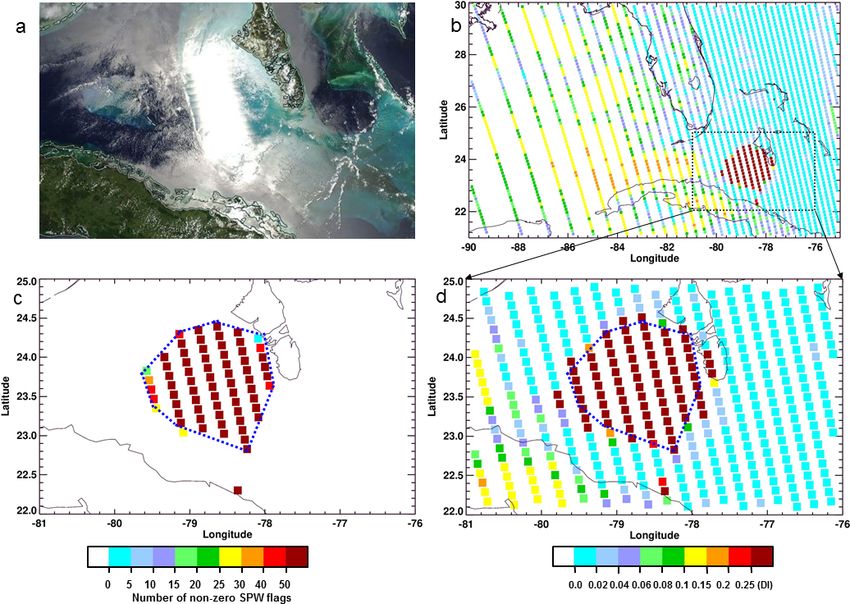
962                                              N. Gorkavyi et al.: Detection of anomalies in the reflectances from the OMI

sor (S5P) satellite, Ozone Mapping and Profiler Suite/Nadir         et al., 2019). TROPOMI also experiences detector saturation
Mapper (OMPS/NM) on the Suomi National Polar-Orbiting               and blooming problems, typically caused by bright tropical
Partnership (Suomi NPP) and National Oceanic and Atmo-              clouds seen in bands 4 (400–499 nm) and 6 (725–786 nm).
spheric Administration (NOAA)-20, and Global Ozone Mon-             Bands 7 (2300–2343 nm) and 8 (2342–2389 nm) react mostly
itoring Experiment 2 (GOME-2) instruments on European               negatively to sunglint. Currently, blooming areas are not de-
Organisation for the Exploitation of Meteorological Satel-          tected by the TROPOMI L0–1b processor. A flagging algo-
lites (EUMETSAT) MetOp platforms.                                   rithm is under development (Rozemeijer and Kleipool, 2019;
   Non-linear effects can impact the measured signal when           Ludewig et al., 2019).
not properly corrected. This can degrade Earthshine radiance           A set of 16 operational flags, called the saturation possi-
measurements from passive solar backscatter UV–vis satel-           bility warning (SPW) flags, is currently included in the OMI
lite spectra and thus impact retrievals of atmospheric con-         level-1b data set. SPWs are designed to flag OMI pixels with
stituents and surface properties. There are several potential       16 various radiation anomalies (e.g., saturation, stray light,
sources for these effects. Saturation occurs when bright light      non-linearity). These flags are defined for each OMI wave-
causes the number of electrons in a sensor pixel to exceed          length: 751 wavelengths of the vis spectrum and 557 wave-
either the maximum charge capacity of an individual charge-         lengths of the UV2 spectrum (GDPS, 2006). All of the 16
coupled device (CCD) photodiode or the maximum charge               SPW flags are binary; a pixel with any degree of abnormality
transfer capacity of the sensor. Blooming and other artifacts       (e.g., saturation) at a given wavelength is marked as possibly
related to charge transfer on the CCD may also affect the           bad.
quality of the measured spectrum when electrons from a satu-           Here, we describe a new approach to identify potentially
rated pixel overflow to a neighboring pixel, causing distortion     erroneous OMI data based on the correlation r between
of its signal and frequently rendering affected data useless.       the observed backscattered Earthshine spectrum and a ref-
Charge transfer and readout errors can also result in a dis-        erence solar spectrum computed over limited spectral re-
torted spectra, as can be the case with an error in correction      gions. Earthshine spectra differ from the solar spectra due
for detector smear. Hereafter, we refer to the spatial domain       to Rayleigh, rotational Raman, aerosol and surface scatter-
of the two-dimensional CCD as rows (30 or 60 simultane-             ing, as well as absorption of radiation by ozone and other
ously acquired scenes) and the spectral domain as columns.          atmospheric components. Most of these factors, with the ex-
Per OMI design, the CCD readout is in spatial pixels more           ception of strong ozone absorption in the UV, amount to sec-
easily, and therefore the blooming or charge readout-related        ondary effects on the correlation coefficient between the so-
effects are expected to predominantly occur between differ-         lar and Earthshine spectra within a limited spectral window.
ent spatial rows.                                                   Under normal conditions (lack of detectable instrument-
   Retrievals of atmospheric gases or aerosols can be com-          imposed spectral distortions) and for a reasonably narrow
promised when observing very bright surfaces such as                (5–10 nm, for practical purposes, with a moderate-resolution
sunglint in low-wind-speed conditions (Cox and Munk,                spectral instrument) spectral window, the degree of correla-
1954; Kay et al., 2009; Butz et al., 2013; Feng et al., 2017), as   tion depends mainly (but not exclusively) on the number and
well as over scenes predominantly covered by optically thick        strength (depth) of solar Fraunhofer features, once we take
clouds. Saturation caused by sunglint routinely occurs in the       into consideration additional factors (differences in spectral
visible imagery of the MODerate Resolution Imaging Spec-            resolution, finite signal-to-noise ratio of measurements, mis-
troradiometer (MODIS) flying on NASA’s Aqua and Terra               alignment of the wavelength grids, among others) that tend
satellites. MODIS data show a gradual increase of saturated         to degrade the correlation. In the windows with well-defined
data towards the red and near-infrared (NIR) bands, reach-          solar absorption spectral features, the correlation coefficient
ing around 1500 pixels, or ∼ 0.03 % of pixels, in a granule at      may gradually approach unity for the scenes acquired with
869 nm (Singh and Shanmugam, 2014). The Orbiting Carbon             S/N  100 – a condition met in a majority of OMI UV2–vis
Observatory-2 (OCO-2) and similar greenhouse gas monitor-           reflectance spectra. Assuming the radiances and irradiances
ing instruments occasionally point directly at the sunglint.        have the same spectral resolution and comparable S/N , and
The OCO-2 in-orbit checkout activities revealed an unex-            are closely co-aligned in the wavelength domain, the correla-
pectedly high signal from Lake Maracaibo, Venezuela, on             tion coefficient between the Earthshine and the solar “etalon”
7 August 2014. This signal saturated all three channels and         (assumed to be distortion free) should be highly sensitive to
was attributed to an oil slick on a wave-free lake. After this      any distortions in the former, leading to rapidly decreasing
event, known as the “Lake Maracaibo saturation incident”,           correlation in saturated scenes (solar glint or bright clouds)
an automated saturation warning algorithm was incorporated          or under other anomalous conditions, such as cosmic-ray hits
into the OCO-2 processing to identify such events (Crisp            on the detector.
et al., 2017). Solar glint from ocean and clouds, as well as           We apply our approach to OMI data and analyze individ-
“saturation tails” or blooming effects are seen in many im-         ual cases and global distributions of flagged data. While these
ages from the Earth Polychromatic Imaging Camera on the             effects have been known for some time and dealt with, to
Deep Space Climate Observatory (EPIC/DSCOVR) (Varnai                some extent, the prevalence of the different effects globally

Atmos. Meas. Tech., 14, 961–974, 2021                                                 https://doi.org/10.5194/amt-14-961-2021
N. Gorkavyi et al.: Detection of anomalies in the reflectances from the OMI                                                  963

for a particular instrument has rarely been documented. This     coefficient:
work provides a detailed analysis of spectrum-distorting ef-                              n
                                                                                          P
fects in the OMI case, as well as a general and straightfor-                             (xi − x) (yi − y)
ward approach that may be applied to similar instruments                                  i=1
                                                                 DI = 1 − r = 1 − s             s               ,            (1)
(TROPOMI, OMPS, GOME-2, etc.) to identify and filter out                            n
                                                                                    P         2 P
                                                                                                   n
                                                                                                              2
suspect or erroneous data.                                                            (xi − x)        (yi − y)
                                                                                       i=1            i=1

                                                                 with x (same for y)
2     Data and methods
                                                                         n
                                                                      1X
2.1    The Ozone Monitoring Instrument                           x=         xi .                                             (2)
                                                                      n i=1
The Aura satellite that hosts OMI is in a polar Sun-
synchronous orbit with a local Equator crossing time of          In Eqs. (1) and (2), xi and yi are the individual sample points
13:45 LT. OMI is a nadir-looking, pushbroom UV–vis grat-         for radiance I and irradiance F0 , respectively. DI is derived
ing spectrometer (Levelt et al., 2018). The light entering the   for radiances and irradiances at each spectral region: for
telescope is depolarized using a scrambler and then split into   OMI, 14 regions of ∼ 10 nm (n = 51 wavelengths for each
two channels: the UV (wavelength range 264–383 nm) and           spectral region) in the vis channel and six regions of ∼ 10 nm
the vis (wavelength range 349–504 nm; Dobber et al., 2006;       (n = 69 wavelengths for each region) in UV2. For the stan-
Schenkeveld et al., 2017). The UV channel is further divided     dard solar spectrum or reference irradiance, we take an av-
into the two subchannels: UV1 (264–311 nm, 0.63 nm reso-         erage of all solar spectra obtained by OMI in 2005. Each
lution and 0.21 nm sampling) and UV2 (307–383 nm range,          Earthshine spectrum is regridded via linear interpolation to
0.42 nm resolution with 0.14 nm sampling). Measurements          match the wavelengths of the averaged irradiance spectrum.
are collected on two-dimensional CCD sensors used for the        An exact match between the radiance and irradiance spectral
UV and vis channels. Spectral information is dispersed along     features gives a DI of 0, whereas when the features in the
one dimension of each CCD and spatial is imaged on the           radiance and irradiance spectra deviate, the DI approaches
other. Each channel has a devoted frame-transfer CCD detec-      1 to 2, where values greater than 1 indicate that irradiance
tor with 6 × 10⁵ electrons/pixel full-well capacity. To avoid    and radiance spectra exhibit anti-correlation. Hence, cases of
blooming and ellipsoid effects, the pixel filling should be      DI > 0 may indicate distortions of atmospheric spectra. Ev-
kept below 3 × 10⁵ electrons (Dobber et al., 2006). OMI also     idently, DI is 0 for the simple case of a perfect match with
measures the solar irradiance once per day through the so-       I = const × F0 ; if I = −const × F0 , then DI is 2. If I and
lar port. Here, we use the UV2 subchannel and vis channel        F0 are completely unrelated, then DI is 1. Considering the
only; in the UV1 channel, strong, variable ozone absorption      “smooth” (low-frequency) component of I and F0 , we ex-
renders our approach impractical.                                pect them to be generally correlated in the spectral regions
    In the global mode, each orbit spans the pole-to-pole sun-   relatively free of major atmospheric absorptions (ozone in
lit portion, typically comprising 1644 along-orbit exposures,    particular). The correlation would be inevitably diminished
referred to as iTimes hereafter. The 114◦ viewing angle of       by the wavelength-dependent Rayleigh scattering and sur-
the telescope corresponds to a 2600 km wide swath on the         face reflectivity. Once a multitude of deep spectral lines is
Earth’s surface and consists of 60 simultaneously acquired       superimposed on a smooth envelope, DI will depend mainly
rows or ground pixels across the track. In this mode, the OMI    on a match between the shape and position of these I and
pixel size is 13 × 24 km2 at nadir. The in-flight performance    F0 spectral transitions, with the correlation depending on the
of OMI is discussed in Schenkeveld et al. (2017). The radio-     S/N of the tested radiances and irradiances, and even more
metric degradation of the OMI radiances since launch ranges      so on slight (in OMI’s case) wavelength misalignments be-
from ∼ 2 % in the UV channel to ∼ 0.5 % in the vis channel,      tween radiances and irradiances, with the steep line flanks
which is much lower than any similar sensor (Levelt et al.,      magnifying the differences.
2018). One major anomaly has occurred with OMI, the so-             An additional decorrelating factor is brought forth by the
called row anomaly (Schenkeveld et al., 2017); it is presum-     omnipresent atmospheric rotational Raman scattering (e.g.,
ably caused by a partial detachment of insulation material       Joiner et al., 1995). Under the circumstances, one may never
exterior to the instrument and produces a number of anoma-       expect DI of 0, save the exceedingly rare cases of a perfect
lous effects on Sun-normalized radiances. The row anomaly        solar glint. It is known that Pearson’s correlation coefficient
is discussed in detail in Sect. 3.4.                             is sensitive to outliers, thus simplifying detection of spectral
                                                                 distortions in the high-resolution data compared to the low-
2.2    The decorrelation index (DI)                              resolution cases, with the latter tending to lessen the impact
                                                                 of additive components (the shallower lines are potentially
We introduce a new parameter, the decorrelation index (DI),      less susceptible to stray light), as well as the wavelength mis-
which is defined as 1 − r, where r is the Pearson correlation    alignment (spectral blending of multiple features leading to

https://doi.org/10.5194/amt-14-961-2021                                                Atmos. Meas. Tech., 14, 961–974, 2021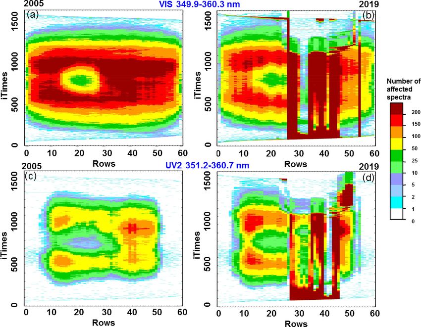
964                                               N. Gorkavyi et al.: Detection of anomalies in the reflectances from the OMI

partial canceling of distortions in the adjacent features). At a     orbit and for every spectral window, we constructed DI his-
given spectral resolution and S/N, DI sensitivity may grow           tograms. Then we selected numerous cases sampling the tails
with increasing numbers and contrasts (depths) of spectral           of the DI histograms. On a case-by-case basis, for differ-
features in the chosen spectral window. At the same time,            ent scenes and spectral windows, we found empirically the
the DI is expected to be sensitive to artifacts associated with      lowest DI values that repeatedly separate the scenes with ap-
cosmic-ray hits. The interval 440–480 nm, where there are            parently normal (spectrally smooth, with the fine-structure,
few deep spectral lines, should be especially sensitive to geo-      low-amplitude Raman-scattering features) and distorted re-
physical factors, for example, to the wavelength-dependent           flectances. These DI thresholds approximately correspond to
albedo of the Earth’s surface. Note that there are cases when        the 99.995–99.998 percentiles in the DI distributions. We
direct solar radiation F0 is mixed with I due to instrument          plan to provide a statistically rigorous threshold definition
problems (see below). Under this specific circumstance, DI           in the improved DI version.
will decrease, since correlation between (I + δF0 ) and F0 is           Table 1 summarizes the DI wavelength bands and sug-
always higher (thus, DI is lower) than between I and F0 . A          gested threshold values corresponding to damaged spectra.
similar effect occurs with sunglint from the water surface,          These critical values should be treated as indicative. A user
when the proportion of directly reflected sunlight in I in-          may define different thresholds depending on their applica-
creases significantly. Note that in the current approach we          tion. We chose row 20 to determine these critical values. The
do not compensate for the relatively smooth spectral differ-         dependence of the threshold DI values on cross-track posi-
ences imposed by atmospheric (Rayleigh scattering) and sur-          tion is relatively minor, except for the first UV2 interval.
face (wavelength-dependent albedo) factors, leaving this to          For this interval, other cross-track positions may carry dif-
the next DI version. This step would make DI more sensitive          ferent values, primarily due to ozone absorption (increasing
to the instrument-imposed anomalies, further disentangling           towards the swath edges). The DI thresholds depend on spec-
those from the geophysical factors (see below).                      tral resolution and S/N of the reflectances; hence, the indica-
   In this initial version of the OMI DI, we use the spectral        tive values from Table 1 may vary for different instruments.
range 309.9–370.0 nm for UV2 and 349.9–498.4 nm for vis.
Overlapping of these ranges is useful for assessing the cali-
bration between the UV2 and VIS channels. For solar zenith           3     Results
angles (SZAs) > 90◦ , the radiance level drops, noise begins
to dominate, and the DI grows rapidly. Therefore, we avoid           To study the DI, we first concentrate on scenes that are most
SZA > 90◦ cases. The DI is sensitive to the degree of dis-           likely to contain saturation effects: sunglint areas with rela-
tortion of the reflectance spectrum, regardless of the cause         tively calm water surfaces and contiguous bands of deep con-
of the distortion (saturation, crosstalk, noise, etc.), so that it   vective clouds. Next, we examine the global DI distribution,
detects distortions other than saturation. For example, the DI       which reveals other effects that damage observed spectra. We
may detect electronic cross-talk (or blooming) effects in pix-       then investigate the impact of the row anomaly on the DI.
els adjacent to the saturated area. In a number of cases, the
DI proves to be either more or less sensitive than the current       3.1    Saturation over clouds
SPW flags reported in the OMI pixel quality flags filed of the
level-1b data, as shown in the next section.                         A typical problematic cluster of bright clouds in the Pacific
   The DI provides a range of values that describes the devi-        Ocean is shown in Fig. 1a, where two zones are highlighted,
ation of observed spectra from the reference irradiance spec-        a small northern zone (denoted A) and a large southern zone
trum, while the SPW flag is a binary value. The DI therefore         (marked as B). Figure 1c shows the number of wavelengths
allows flexibility in setting detection thresholds for damaged       for a given pixel marked with the SPW flag as saturated. Fig-
spectra for different applications. The DI value for a given         ure 1b–d show the corresponding DI values for the vis in-
spectral interval depends strongly on the number of Fraun-           terval at 414–424 nm. The DI indicates that the spectra in
hofer lines as well as presence of strong ozone absorption           zone A are weakly affected, and in zone B they are badly
features within the wavelength range. Therefore, the DI val-         damaged. Figure 1c shows the number of wavelengths for a
ues corresponding to likely damaged spectra vary somewhat            given pixel marked with the SPW flag as saturated.
for each spectral region. For example, the 14 DI divisions of           Figures 2 and 3 illustrate the properties of the DI that char-
the vis spectrum generally fall into two distinct groups; for        acterize the quality of a given part of the spectrum using a
the first group, the value of DI above 0.01–0.03 is a sign of        single parameter. Figure 2 shows an example of a spectrum
a significant distortion of the spectrum, while for the second       with slight distortions that are captured by the SPW flags but
group a typical distortion threshold value is larger (∼ 0.1–         nevertheless has low values of the DI. Small deviations of
0.4). The provisional (the user may redefine the values us-          the DI from 0 can result from geophysical effects, for exam-
ing the auxiliary data provided in the OMI DI product) DI            ple, an increased amount of ozone, and minor damage to the
thresholds were determined as follows. We used all avail-            spectrum, as shown in Fig. 2. Those users who have strict re-
able, mission-long OMI UV2 and vis radiances. For each               quirements for the quality of the spectra should use the SPW

Atmos. Meas. Tech., 14, 961–974, 2021                                                   https://doi.org/10.5194/amt-14-961-2021
N. Gorkavyi et al.: Detection of anomalies in the reflectances from the OMI 965
Table 1. Chosen OMI DI spectral intervals and indicative DI thresholds for damaged spectra.
Interval Wavelengths (nm) Value DI as signature of Comments
(UV2) (for row 20) distortion of spectra
1 309.94–320.61 –∗ Strong ozone effects
2 320.76–331.08 > 0.20–0.25 Ozone effects
3 331.23–341.24 > 0.35–0.45 Weak ozone effects
4 341.39–351.11 > 0.02–0.03 Strong spectral lines
5 351.25–360.70 > 0.02 Strong spectral lines
6 360.84–370.02 > 0.01 Strong spectral lines
(vis)
1 349.93–360.33 > 0.03 Strong spectral lines
2 360.54–370.93 > 0.01 Strong spectral lines
3 371.14–381.52 > 0.02 Strong spectral lines
4 381.73–392.11 > 0.01 Strong spectral lines
5 392.32–402.70 > 0.01 Strong spectral lines
6 402.91–413.29 > 0.06–0.08
7 413.50–423.89 > 0.1–0.15
8 424.10–434.50 > 0.02–0.03 Strong spectral lines
9 434.71–445.12 > 0.05–0.1
10 445.32–455.74 > 0.25
11 455.95–466.39 > 0.4
12 466.60–477.05 > 0.4
13 477.26–487.72 > 0.03 Strong spectral lines
14 487.93–498.41 > 0.2
∗ The threshold depends on the row number.
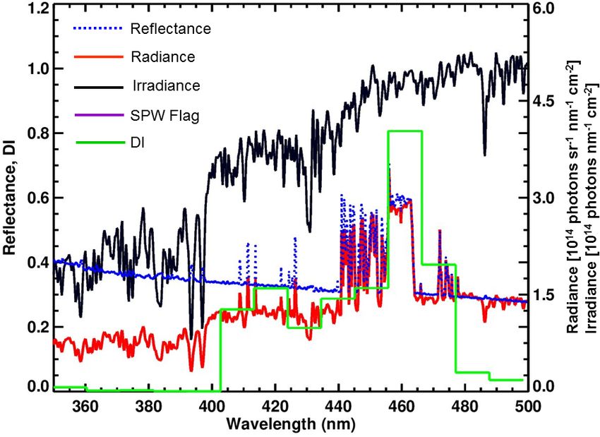
flag in this case, which detects minor damage to the spec- 3.2 Saturation over lakes and oceans
trum. Figure 3 shows the vis spectrum for a pixel in zone B
(indicated by an arrow in Fig. 1) corresponding to iTimes
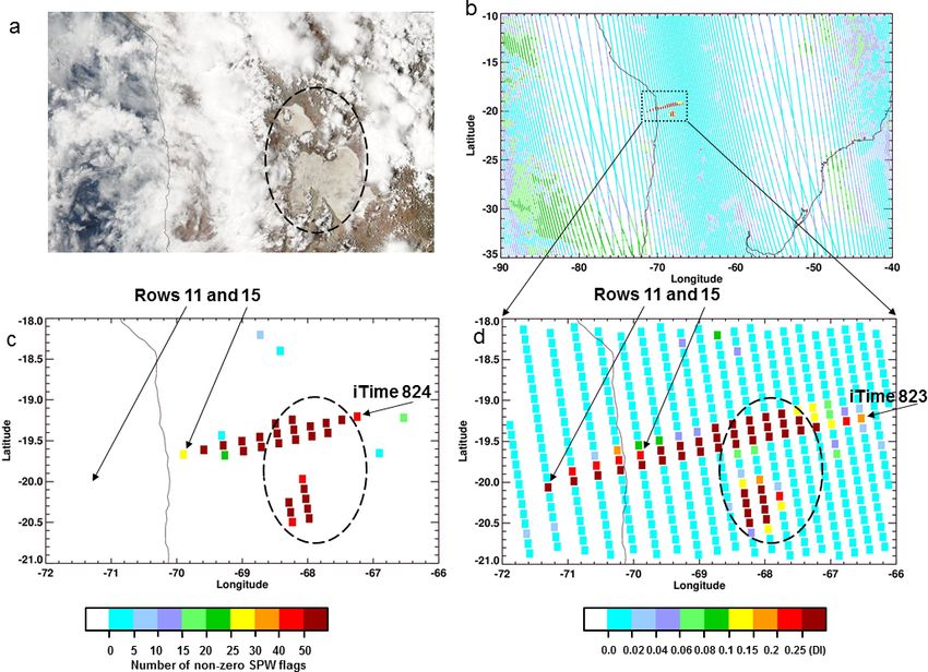
807, row 20. The radiance spectrum is saturated in the 400– The South American Salar de Uyuni is a lake used for cal-
465 nm range. In contrast to Fig. 2, damage in this spectrum ibration of many satellite sensors (Lamparelli et al., 2003;
is manifested in both the SPW flag and the DIs. The DIs re- Fricker et al., 2005). Salar de Uyuni is dry for most months
flect the degree of spectral damage, which in this case reaches of the year, but during the rainy season, it is filled with shal-
a maximum near 450 nm. Based on the problem studied here, low water with strong direct reflectance from the Sun. This
a user can determine whether the spectrum is useful despite may cause saturation of OMI’s detectors. The lake, covered
minor damage such as in zone A. In such cases, the SPW and with shallow water, generated strong solar glint, for exam-
DI may provide complementary information. ple, for orbit 7987 (14 January 2006). Figure 4a shows this
Reflectance in Figs. 2 and 3 is defined as π ·I /[F0 ·cos(θ )], shallow lake on 14 January 2006 as observed by the Aqua
where I is the top-of-the-atmosphere (TOA) radiance, F0 is MODIS sensor. The SPW flags (Fig. 4c) and DIs (Fig. 4b, d)
the extraterrestrial solar flux, and θ is the SZA. Usually, the for this case show that the lake generates two bright spots:
wavelength dependence of TOA reflectance is fairly smooth, southern and northern. The solar glint from the northern spot
albeit with relatively low-amplitude, high-frequency struc- is so bright that the signal extends to nearby pixels (iTimes
tures due to rotational Raman scattering, also known as the 823–825, rows 11–14) and is detected by the DI (see also
Ring effect. Both zones in Fig. 1 have high values of re- Cao et al., 2019; Shen et al., 2019, for examples of bloom-
flectance; for zone A, reflectance is between 0.95 and 1.0 ing in other sensors). The SPW flags are unset for significant
(Fig. 2), while for zone B, reflectance is between 1.0 and 1.1 portions of the affected OMI pixels (see Fig. 4).
(Fig. 3). In some viewing directions, the reflectance can ex- Figure 5 shows the vis spectrum for a pixel on the edge
ceed unity due to anisotropic angular distribution of the TOA of the highly saturated region. This pixel may have super-
radiance. imposed effects of moderate saturation of the pixel itself as
well as charge overflow from due to significant saturation in
the neighboring pixels (iTimes 824, row 15). While the re-
flectance values of many of these pixels (rows ∼ 11–15 in
Fig. 4) are in the expected range (0.3–0.6), there are numer-
https://doi.org/10.5194/amt-14-961-2021 Atmos. Meas. Tech., 14, 961–974, 2021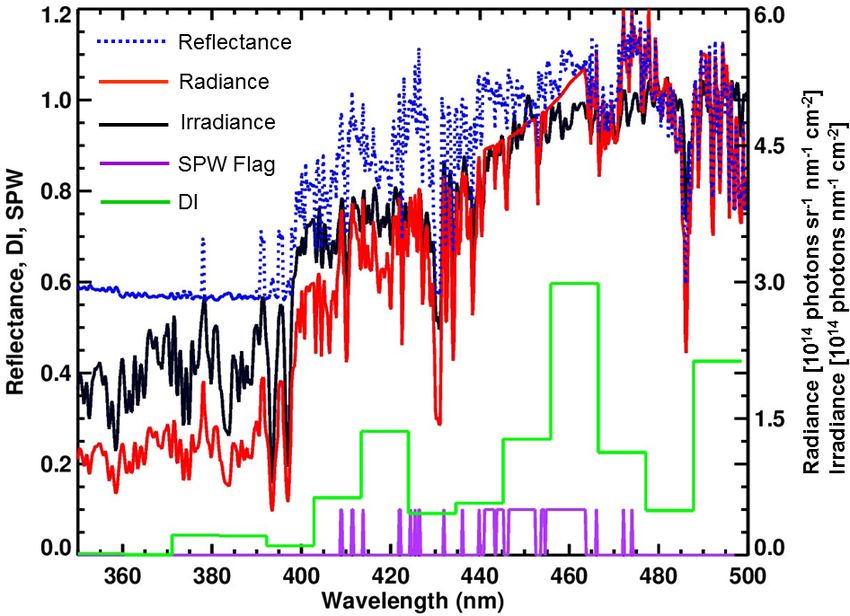
966                                              N. Gorkavyi et al.: Detection of anomalies in the reflectances from the OMI

Figure 1. Two cloud zones in the south Pacific on 14 January 2006 for orbit 7990: small northern zone labeled “A” and large southern
labeled “B” (a) Aqua MODIS image; (b, d) DI maps for the vis spectral region (414–424 nm); (c) the number of wavelengths for a given
pixel marked with the SPW flag as saturated (the maximum number is 51 in this vis spectral region).

ous cases where the final radiance signal is well beyond nor-       thus forming a “smile”. This may result in occasional aug-
mal range, thus leading to high DIs.                                mented distortions around narrow, well-defined features in
   Figure 6 shows the spectrum of a pixel where the prevail-        the spectral image in non-saturated pixels, while the signal
ing anomalous effect do not appear to be direct saturation          for other wavelengths in the spectrum may remain intact.
(iTimes 824, row 11). High DI values are seen for a number          Such occasional distortions could be mimicked and greatly
of corrupted parts of the spectrum where the SPW flags are          outnumbered by a different effect that also stems from the
zero. While the saturated case is straightforward to detect and     spectral smile. In some cases, brightly lit (but not saturated)
interpret (e.g., the practically featureless radiances in Figs. 3   scenes border low-reflectance areas: e.g., the studied Salar de
and 4), these other spectral distortions may have a complex         Uyuni case, cloud-front edges or the edges of extended fresh
spectral envelope due to the differences in the wavelength          snow and/or ice fields. In these bordering low-reflectance
sampling of the sequential OMI rows.                                scenes, the greatly augmented spatial stray light could mimic
   The completely saturated spectral domains may trigger            a blooming effect caused by the spectral smile, thus lead-
effects in the neighboring rows, indiscriminately affecting         ing to higher DI around strong, deep spectral transitions that
the involved wavelengths. However, in the case of a less            may exceed the imposed threshold. In the OMI data sampling
severely saturated scene, there might be additional effects to      the high-contrast scenes, the spatial stray-light effects induce
consider. Per instrument design, the OMI wavelength grids           wavelength shifts that affect trace-gas retrievals (Richter et
form a “spectral smile” in the row-wise direction. Inspect-         al., 2020). Some of the above-threshold DIs in the global
ing the wavelength registration for a given CCD column (the         maps (midlatitudes to high latitudes, open-water scenes; see
spectral domain) while moving from the swath’s edges to-            below) could be triggered by the high-contrast scenario.
wards nadir, one may notice gradual wavelength shifts be-              An example of solar glint in the Caribbean Sea is shown in
tween the adjacent rows. The wavelengths are increasing             Fig. 7 for 26 July 2013. Effects of the glint for this case are
while moving from the edges to the center of the swath,             detected in both the DI and SPW flags. Some of the pixels

Atmos. Meas. Tech., 14, 961–974, 2021                                                  https://doi.org/10.5194/amt-14-961-2021
N. Gorkavyi et al.: Detection of anomalies in the reflectances from the OMI 967
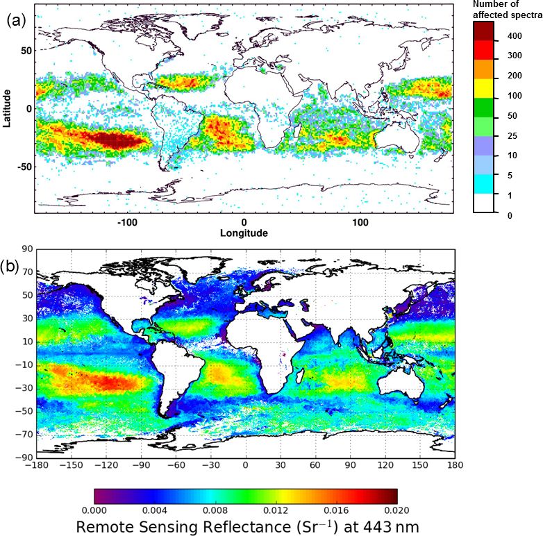
The global DI behavior depends on many geophysical and in-
strumental processes. For example, Fig. 8a shows the spatial
distribution of the number of spectra with DI > 0.03 for the
424.1–434.5 nm range. Figure 8b similarly shows distribu-
tions for DI > 0.25 in the 445.3–455.7 nm spectral window.
Despite the different threshold DI values that characterize the
distorted spectra, these two DIs show similar distributions of
corrupted spectra associated with enhanced cosmic-ray hits
on the detectors within the South Atlantic Anomaly (SAA)
region, glint and a solar eclipse zone. Though we cannot dis-
entangle the contributing factors for the latter, here we men-
tion two of them as the likely causes of the high DI values
(thus enhanced distortions in the reflectances): the low S/N
of the eclipsed radiances, as well as the drastically increased
portion (compared to the normally lit scenes) of the additive
(stray-light) component.
Figure 2. Data for iTimes 839, row 15, orbit 7990, 14 January 2006
The interpretation of low DI for normal spectra (for ex-
in zone A (this pixel is marked by arrows in Fig. 1c, d). The blue line
at the top of the picture is reflectance πI /[F0 cos(θ)], where θ is so- ample, spectra with DI > 0.1 for vis of 445.3–455.7 nm) is
lar zenith angle. Reflectance in this zone has slight variations caused quite complicated as low DI values depend on many fac-
by minor saturation in the atmospheric spectrum, as indicated by the tors. Figure 9 shows the spatial distribution of the number
arrows. The purple line shows the binary SPW flags multiplied by of spectra with DI > 0.1 in the 445.3–455.7 nm region com-
0.1. The green line is the DI < 0.01 for bands 403–413, 413–424 pared with ocean reflectance at 443 nm. There is obvious
and 424–434 nm. The intensity of the radiance spectrum is shifted spatial correlation between the spectra the DI identifies and
upwards slightly for clearer comparison with the irradiance spec- ocean reflectance: larger numbers of such spectra correspond
trum. to ocean areas with higher reflectance. This is particularly
pronounced in the southern Pacific gyre whose waters ex-
hibit extremely low bioproductivity and thus are very bright
in the blue region (Tedetti et al., 2007). The strong spectral
dependence of water-leaving reflectance in the blue region in
these extremely clear waters results in lower correlation with
the solar spectrum. This may be attributed in part to vibra-
tional Raman scattering that is prevalent in clear ocean wa-
ters (Vasilkov et al., 2002; Westberry et al., 2013). Addition-
ally, the Pacific gyre area is characterized by low cloudiness
and low aerosol loadings. Therefore, in this area, the rela-
tively high proportion of the shown data comes from the sur-
face, thus being more susceptible to the Rayleigh and Raman
scattering effects. These change the TOA radiances in differ-
ent ways: the low-frequency spectral envelope is affected by
Rayleigh, while the fine-scale structures are introduced by
the vibrational and rotational Raman scattering. Both effects
Figure 3. Similar to Fig. 2 but for iTimes 807, row 20, orbit 7990,
lead to “distorted” reflectances and thus higher DIs.
14 January 2006 in cloud region B (see arrows in Fig. 1c, d). The Figure 10a–b show the orbital distributions of the 445.3–
radiance was lowered by a few percent for better comparison. 455.7 nm DI for DI > 0.25 and DI > 0.6 , respectively, plot-
ted for OMI detector rows (generally oriented east–west
across the satellite track) versus iTimes (north–south orbital
not marked by the SPW flags show high DI values that may direction) for 2006. A block of 250 along-orbit exposures
be related to blooming or other effects associated with the (iTimes) approximately covers 30◦ in latitude. The middle
impaired performance of neighboring pixels on the detector. of this band falls on the Equator on 22 March. During the
year, this band shifts by 22.4◦ to both the north and south.
3.3 Orbital and global distribution The zone around row 21 and iTimes 820 is an area of solar
glint from the ocean surface (case where DI > 0.6; Fig. 10b)
Figures 8–10 show global distributions of the number of af- that does not change with season. The distribution of bright
fected vis spectra with DI greater than thresholds for spectra clouds with DI > 0.25 also shows a strong propensity for the
for March 2006 (Figs. 8 and 9) and for all of 2006 (Fig. 10). geometrical conditions of solar glint (Fig. 10a). This is con-
https://doi.org/10.5194/amt-14-961-2021 Atmos. Meas. Tech., 14, 961–974, 2021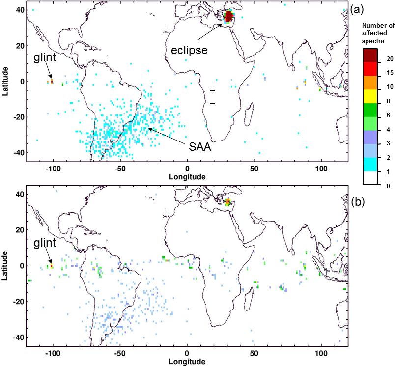
968                                                 N. Gorkavyi et al.: Detection of anomalies in the reflectances from the OMI

Figure 4. Similar to Fig. 1 but for an area near Salar de Uyuni, 14 January 2006, orbit 7987.

Figure 5. Similar to Fig. 2 but for pixel iTimes 824, row 15, orbit      Figure 6. Similar to Fig. 5 but for pixel iTimes 823, row 11, orbit
7987 indicated by arrows in Fig. 4c, d showing solar glint from Salar    7987 (see arrows in Fig. 4d). SPW flags are zero for this case and
de Uyuni.                                                                are not shown.

Atmos. Meas. Tech., 14, 961–974, 2021                                                           https://doi.org/10.5194/amt-14-961-2021
N. Gorkavyi et al.: Detection of anomalies in the reflectances from the OMI 969
Figure 7. Similar to Fig. 1 but for an area showing solar glint near the Bahamas (orbit 48034, 26 July 2013). Glint positions in panels (c)
and (d) do not exactly match those in the RGB image (a). The area of pixels marked by the SPW flags are approximately delineated by the
dotted blue line.
sistent with EPIC/DSCOVR data showing solar glint from a complex phenomenon that may result in artificially low or
clouds that contain oriented ice plates (Varnai et al., 2019). high values of reflectances, additionally affecting their wave-
In the OMI case, the strongly saturated (or damaged) spectra length dependence. The RA stems from an interplay of mul-
with DI > 0.60 occur at a rate of about 2500 (∼ 0.0005 %) or tiple factors that may affect the DI values. The RA is likely
∼ 7 spectra d−1 . Slightly affected spectra (0.25 < DI < 0.6) linked to a gradual detachment of the thermal blanket par-
occur at a rate of ∼ 0.002 % or ∼ 33 spectra d−1 . tially blocking some fields of view (FOVs) (rows). Since
this blanket is highly reflective, its warped surface causes
3.4 The row anomaly occasional (solar-angle dependent, predominantly affecting
northern portion of the OMI orbit) reflection of the direct
sunlight into some RA-affected rows. In addition, the re-
The row anomaly (RA) renders a significant portion of the
flective surface leads to enhanced spatial cross-talk between
OMI rows as unusable. The anomaly was clearly detected
adjacent RA-affected scenes (an anomalous stray light that
in two rows in June 2007. In May 2008, the row anomaly
is regulated by the wavelength- and angle-dependent reflec-
spread to several other rows on the sensor. The row anomaly
tivity of the blanket). The time-, space- and wavelength-
has continued to develop since then, with particularly swift
dependent combination of three factors may lead to in-
changes around January 2009 and early fall of 2011. Cur-
creasing or decreasing DIs. Even more complications stem
rently, about 33 % of the UV2 rows are affected in the South-
from the fact that the RA may increase inhomogeneity of
ern Hemisphere parts of the OMI orbit. This increases to
the spectral-slit illumination, thus causing substantial (and
∼ 57 % in the Northern Hemisphere. These estimates are
unaccounted-for) wavelength shifts and ensuing spectral dis-
comparable in the vis channels (Schenkeveld et al., 2017).
tortions in the reflectances.
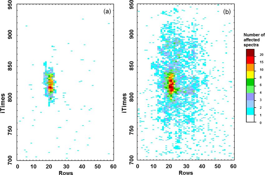
Figure 11 shows DI distributions in the row versus iTimes
Deciphering the complex RA-related patterns in Fig. 11,
format (traditionally used for RA tracking) for the overlap-
we first of all relate them to the pre-RA epoch that shows
ping region of the UV2 and vis detectors. The row anomaly is
https://doi.org/10.5194/amt-14-961-2021 Atmos. Meas. Tech., 14, 961–974, 2021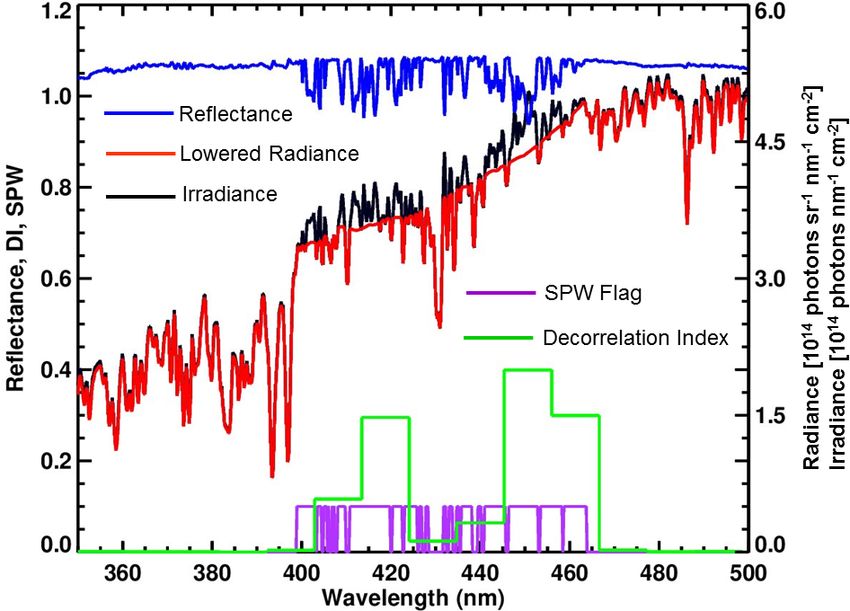
970                                                N. Gorkavyi et al.: Detection of anomalies in the reflectances from the OMI

Figure 8. Gridded (1◦ × 1◦ ) distributions of the number of affected spectra for March 2006; (a) vis of 424.1–434.5 nm, DI > 0.03; (b) vis of
445.3–455.7 nm, DI > 0.25. The South Atlantic Anomaly and a region affected by solar eclipse are clearly visible; the remaining pixels with
high DI values are mostly associated with sunglint and bright clouds.

an increase in the above-threshold cases in the equatorial re-           responding DIs. The solar influence appears to be strongly
gions, with a pronounced minimum centered on the sunglint                cross-swath modulated. This is a new aspect that requires
domain (rows 10–30 and iTimes∼ 650–1000). At the same                    a detailed follow-up study that is beyond the scope of the
time, the numbers of the above-threshold cases diminish to-              paper. At the same time, the remainder of the RA-affected
wards the higher latitudes and OMI’s swath edges. In the                 areas show significant increase in the above-threshold DIs.
TOA reflectances coming from the sunglint areas, the higher              This likely comes from the RA-imposed and unaccounted-
proportion of the directly reflected sunlight leads to a higher          for wavelength shifts.
radiance–irradiance correlation and thus lower DIs. The lat-                The lower DI counts in the sunglint areas in Fig. 11 seem-
itudinal and swath-angle-dependent trends can be linked to               ingly contrast with the increased DI values at the center
the gradually diminished influence of the surface that modu-             of these regions in the vis (Fig. 10). One should note that
lates the TOA reflectances due to the wavelength-dependent               Figs. 10 and 11 sample different spectral domains, with the
surface albedos. In the planned upgrade of the DI algorithm,             445.3–455.7 nm range (Fig. 10) known to be highly suscep-
we intend to address this component, thus decreasing the im-             tible to saturation, contrary to the exceedingly rare incidence
pact of geophysical factors.                                             of saturation in the 349.9–360.3 nm band (Fig. 11).
   Turning our attention to the RA-affected areas in Fig. 11,
we notice that DIs closely delineate the RA-affected areas
and show pronounced north–south asymmetry, with intricate                4   Discussion and conclusions
patterns of the relatively higher or lower DIs compared to
the RA-free plots. The north–south asymmetry is caused by                The OMI pixel quality flags (PQFs) were designed to char-
the well-documented northward growth (Schenkeveld et al.,                acterize each wavelength of the OMI spectrum (SPW flag is
2017) of the blanket-reflected direct-sunlight component in              just one of the 16 bits in the PQF). The DI, developed on the
the RA-affected radiances. This inevitably lessens the cor-              basis of the correlations between observed and solar spec-
                                                                         tra, can serve as a simple but effective and complementary

Atmos. Meas. Tech., 14, 961–974, 2021                                                        https://doi.org/10.5194/amt-14-961-2021
N. Gorkavyi et al.: Detection of anomalies in the reflectances from the OMI 971 Figure 9. (a) Gridded (1◦ × 1◦ ) distribution of a number of spectra with DI > 0.1 for vis of 445.3–455.7 nm in March 2006; (b) ocean remote sensing reflectance for March 2006 at 443 nm from Aqua MODIS. Figure 10. Distribution of a number of affected spectra for 2006, vis of 445.3–455.7 nm; (a) DI > 0.6; (b) DI > 0.25. Usually each pixel collects ∼ 5000 spectra per year. https://doi.org/10.5194/amt-14-961-2021 Atmos. Meas. Tech., 14, 961–974, 2021
972                                                N. Gorkavyi et al.: Detection of anomalies in the reflectances from the OMI

Figure 11. Distribution of the number of affected spectra (DI > 0.01) for March 2005 (a, c) and 2019 (b, d) for vis of 349.9–360.3 nm (a, b)
and UV2 of 351.2–360.7 nm (c, d). The row anomaly is responsible for the stripes of high values shown in 2019.

method for detecting and discarding anomalous UV and vis                rience significant deviations from the solar spectrum due to
satellite spectra, for example, associated with detector satu-          geophysical reasons.
ration, blooming, charge transfer or readout, excessive noise,             The DI can be a useful tool for analyzing spectra ob-
cases of very low reflectance such as solar eclipse or the OMI          tained from other current and future space-borne sensors that
row anomaly. The DI summarizes all changes in the spectrum              may suffer from saturation and blooming such as TROPOMI
in one parameter and eliminates the need to examine all the             (launched in 2017) or the similar Environmental trace gases
available flags for a given pixel. An important motivation for          Monitoring Instrument (EMI) on the GaoFen-5 satellite
introducing such an index is the convenience of handling it.            (Cheng et al., 2019; Ren et al., 2020) (launched in 2018).
For example, to infer enhanced information of the quality of            Similar sensors include the OCO-2 (launched in 2014) and
spectra in the vis region, we introduce 14 scalar-valued DIs            OCO-3 (launched in 2019) (Eldering et al., 2019), South
for regions of the spectrum. For comparison, there are 751              Korea’s geostationary Environment Monitoring Spectrom-
binary saturation flags per spectrum in level 1b. Similarly,            eter (GEMS) (launched 18 February 2020), NASA’s geo-
we use six DIs for the UV2 spectrum, much fewer than the                stationary Tropospheric Emissions: Monitoring of Pollution
577 flags assigned in level 1b. Interpreting a large number of          (TEMPO) (Zoogman et al., 2017) (planned for launch in
flags can be difficult. The DI product gives an indication of           2022), the Copernicus geostationary Sentinel-4 (planned for
spectral quality based on overall correlation that is easier to         launch in 2023) and low-Earth-orbit Sentinel-5 (planned for
interpret. Assessment of the DI with the OMI Collection 3               launch in 2023). Many of these sensors have a smaller pixel
L1b record has motivated improvements in detector correc-               size and/or smaller FOV than OMI. For such instruments,
tions for the next version of the L1b product to be released            this may lead to an increase in the effects of sunglint. Studies
in OMI Collection 4. The continuous nature of the DI allows             utilizing the DI with current instruments may benefit the de-
data users to assign lower confidence to regions of the spectra         sign of future instruments by identifying how often and under
that may not be completely saturated as detected by an elec-            what conditions spectra are impacted by non-linear effects.
tronic saturation algorithm. DI values vary for spectra that
do not experience any anomalies. These variations of the DI
may carry information that can be used for other purposes.              Data availability. The decorrelation index data for OMI Col-
For instance, the DI can be used to search for areas of clear           lection 3 data will be available at the NASA Goddard Earth
ocean water, in which the spectra are not abnormal but expe-            Sciences Data and Information Services Center (GES DISC).
                                                                        The OMI level-1b data used for calculations of the DI are

Atmos. Meas. Tech., 14, 961–974, 2021                                                       https://doi.org/10.5194/amt-14-961-2021
N. Gorkavyi et al.: Detection of anomalies in the reflectances from the OMI 973
available at https://doi.org/10.5067/Aura/OMI/DATA1004 (Dob- and intercomparison with OMI and TROPOMI, Remote Sens.-
ber, 2007a) and https://doi.org/10.5067/Aura/OMI/DATA1002 Basel, 11, 3017, https://doi.org/10.3390/rs11243017, 2019.
(Dobber, 2007b). MODIS data are available at Cox, C. and Munk, W.: Measurement of the roughness of the sea
https://doi.org/10.5067/MODIS/MYD09.006 (Vermote, 2015). surface from photographs of the Sun’s glitter, J. Opt. Soc. Am.,
44, 838–850, https://doi.org/10.1364/JOSA.44.000838, 1954.
Crisp, D., Pollock, H. R., Rosenberg, R., Chapsky, L., Lee, R. A.
Author contributions. NG developed computer codes, analyzed the M., Oyafuso, F. A., Frankenberg, C., O’Dell, C. W., Bruegge, C.
DI results and wrote the manuscript. ZF supported the develop- J., Doran, G. B., Eldering, A., Fisher, B. M., Fu, D., Gunson, M.
ment and implementation of the algorithms and comparison DI R., Mandrake, L., Osterman, G. B., Schwandner, F. M., Sun, K.,
results with the ocean reflectance. DH proposed a concept of DI Taylor, T. E., Wennberg, P. O., and Wunch, D.: The on-orbit per-
and wrote the manuscript. SM proposed a concept of DI and sup- formance of the Orbiting Carbon Observatory-2 (OCO-2) instru-
ported the development and implementation of the algorithms. JJ ment and its radiometrically calibrated products, Atmos. Meas.
set the task of developing an effective method for determining solar Tech., 10, 59–81, https://doi.org/10.5194/amt-10-59-2017, 2017.
glints, supported the development of the algorithm and wrote the Dobber, M.: OMI/Aura Level 1B VIS Global Geolocated
manuscript. AV supported the development of the algorithm and Earth Shine Radiances 1-orbit L2 Swath 13x24 km
wrote the manuscript. V003, Greenbelt, MD, USA, Goddard Earth Sciences
Data and Information Services Center (GES DISC),
https://doi.org/10.5067/Aura/OMI/DATA1004, 2007a.
Competing interests. The authors declare that they have no conflict Dobber, M.: OMI/Aura Level 1B UV Global Geolo-
of interest. cated Earthshine Radiances 1-orbit L2 Swath 13x24
km V003, Greenbelt, MD, USA, Goddard Earth Sci-
ences Data and Information Services Center (GES DISC),
https://doi.org/10.5067/Aura/OMI/DATA1002, 2007b.
Acknowledgements. The authors thank the OMI and MODIS in-
Dobber, M. R., Dirksen, R. J., Levelt, P. F., van den Oord,
strument teams for providing the OMI and MODIS data presented,
G. H. J., Voors, R. H. M., Kleipool, Q., Jaross, G.,
respectively. We acknowledge the use of imagery from the NASA
Kowalewski, M., Hilsenrath, E., Leppelmeier, G. W., de Vries,
Worldview application, part of the NASA Earth Observing System
J., Dierssen, W., and Rozemeijer, N. C.: Ozone Monitoring In-
Data and Information System (EOSDIS).
strument calibration, IEEE T. Geosci. Remote, 44, 1209–1238,
We dedicate this work to the memory of Remco Braak, whose
https://doi.org/10.1109/TGRS.2006.869987, 2006.
early work on saturation in OMI spectra helped to motivate this
Eldering, A., Taylor, T. E., O’Dell, C. W., and Pavlick, R.:
work.
The OCO-3 mission: measurement objectives and expected
performance based on 1 year of simulated data, Atmos.
Meas. Tech., 12, 2341–2370, https://doi.org/10.5194/amt-12-
Financial support. This research has been supported by the NASA 2341-2019, 2019.
Aura project (OMI core team funding) managed by Ken Jucks. Feng, L., Hu, C., Barnes, B. B., Mannino, A., Heidinger, A. K., Stra-
bala, K., and Iraci, L. T.: Cloud and Sun-glint statistics derived
from GOES and MODIS observations over the Intra-Americas
Review statement. This paper was edited by Alexander Sea for GEO-CAPE mission planning, J. Geophys. Res.-Atmos.,
Kokhanovsky and reviewed by two anonymous referees. 122, 1725–1745, https://doi.org/10.1002/2016JD025372, 2017.
Fricker, H. A., Borsa, A., Minster, B., Carabajal, C., Quinn,
K., and Bills., B.: Assessment of ICESat performance at the
Salar de Uyuni, Bolivia, Geophys. Res. Lett., 32, L21S06,
https://doi.org/10.1029/2005GL023423, 2005.
References GDPS: Input/Output Data Specification (IODS) v.
2, Level 1B Output product and Metadata, SD-
Butz, A., Guerlet, S., Hasekamp, O. P., Kuze, A., and Suto, H.: Us- OMIE-7200-DS-467, 44–45, 25 August 2006,
ing ocean-glint scattered sunlight as a diagnostic tool for satel- available at: https://manualzz.com/doc/28490086/
lite remote sensing of greenhouse gases, Atmos. Meas. Tech., 6, gdps-input-output-data-specification--iods--volume-2-leve
2509–2520, https://doi.org/10.5194/amt-6-2509-2013, 2013. (last access: 2 February 2021), 2006.
Cao, X., Hu, Y., Zhu, X., Shi, F., Zhuo, L., and Chen, J.: A sim- Hassinen, S., Tamminen, J., Tanskanen, A., Leppelmeier, G.,
ple self-adjusting model for correcting the blooming effects in Mälkki, A., Koskela, T., Karhu, J. M., Lakkala, K., Veefkind, P.,
DMSP-OLS nighttime light images, Remote Sens. Environ., 224, Krotkov, N., and Aulamo, O.: Description and validation of the
401–411, https://doi.org/10.1016/j.rse.2019.02.019, 2019. OMI very fast delivery products, J. Geophys. Res., 113, D16S35,
Chan Miller, C., Gonzalez Abad, G., Wang, H., Liu, X., Kurosu, https://doi.org/10.1029/2007JD008784, 2008.
T., Jacob, D. J., and Chance, K.: Glyoxal retrieval from the Joiner, J., Bhartia, P. K., Cebula, R. P., Hilsenrath, E., McPeters,
Ozone Monitoring Instrument, Atmos. Meas. Tech., 7, 3891– R. D., and Park, H.: Rotational Raman scattering (Ring effect)
3907, https://doi.org/10.5194/amt-7-3891-2014, 2014. in satellite backscatter ultraviolet measurements, Appl. Opt., 34,
Cheng, L., Tao, J., Valks, P., Yu, Ch., Liu, S., Wang, Y., Xiong, X., 4513–4525, https://doi.org/10.1364/AO.34.004513, 1995.
Wang, Z., and Chen, L.: NO2 retrieval from the Environmen-
tal trace gases Monitoring Instrument (EMI): preliminary results
https://doi.org/10.5194/amt-14-961-2021 Atmos. Meas. Tech., 14, 961–974, 2021974 N. Gorkavyi et al.: Detection of anomalies in the reflectances from the OMI Kay, S., Hedley, J. D., and Lavender, S.: Sun glint correction of high Sellitto, P., Bojkov, B. R., Liu, X., Chance, K., and Del Frate, F.: and low spatial resolution images of aquatic scenes: a review Tropospheric ozone column retrieval at northern mid-latitudes of methods for visible and near-Infrared wavelengths, Remote from the Ozone Monitoring Instrument by means of a neu- Sens., 1, 697–730, https://doi.org/10.3390/rs1040697, 2009. ral network algorithm, Atmos. Meas. Tech., 4, 2375–2388, Krotkov, N. A., Li, C., and Leonard, P.: OMI/Aura sul- https://doi.org/10.5194/amt-4-2375-2011, 2011. phur dioxide (SO2 ) total column L3 1 d best pixel in Shen, Z., Zhu, X., Cao, X., and Chen, J.: Measurement 0.25◦ × 0.25◦ V3, Goddard Earth Sciences Data and In- of blooming effect of DMSP-OLS nighttime light data formation Services Center (GES DISC), Greenbelt, USA, based on NPP-VIIRS data, Ann. GIS, 25, 153–165, https://doi.org/10.5067/Aura/OMI/DATA3008, 2015. https://doi.org/10.1080/19475683.2019.1570336, 2019. Lamparelli, R. A. C., Ponzoni, F. J., Zullo, J., Pellegrino G. Q., and Singh, R. K. and Shanmugam, P.: A robust method for removal Arnaud, Y.: Characterization of the Salar de Uyuni for in-orbit of glint effects from satellite ocean colour imagery, Ocean Sci. satellite calibration, IEEE T. Geosci. Remote, 41, 1461–1468, Discuss., 11, 2791–2829, https://doi.org/10.5194/osd-11-2791- https://doi.org/10.1109/TGRS.2003.810713, 2003. 2014, 2014. Levelt, P. F. (Ed.): OMI instrument description and level 1B prod- Tedetti, M., Sempere, R., Vasilkov, A., Charriere, B., Nerini, D., uct, ATBD-OMI-01, 1 August 2002, available at: https://eospso. Miller, W. L., Rawamura, K., and Raimbault. P.: High penetration nasa.gov/sites/default/files/atbd/ATBD-OMI-01.pdf (last access: of ultraviolet radiation in the south east Pacific waters, Geophys. 2 February 2021), 2002. Res. Lett., 34, L12610, https://doi.org/10.1029/2007GL029823, Levelt, P. F., Joiner, J., Tamminen, J., Veefkind, J. P., Bhartia, P. K., 2007. Stein Zweers, D. C., Duncan, B. N., Streets, D. G., Eskes, H., Varnai, T., Kostinski, A. B., and Marshak, A.: Deep Space Observa- van der A, R., McLinden, C., Fioletov, V., Carn, S., de Laat, J., tions of sun glints from marine ice clouds, IEEE Geosci. Remote DeLand, M., Marchenko, S., McPeters, R., Ziemke, J., Fu, D., S., 17, 735–739, https://doi.org/10.1109/LGRS.2019.2930866, Liu, X., Pickering, K., Apituley, A., González Abad, G., Arola, 2019. A., Boersma, F., Chan Miller, C., Chance, K., de Graaf, M., Vasilkov, A. P., Joiner, J., Gleason, J. F., and Bhartia, P. Hakkarainen, J., Hassinen, S., Ialongo, I., Kleipool, Q., Krotkov, K.: Ocean Raman scattering in satellite backscatter ultra- N., Li, C., Lamsal, L., Newman, P., Nowlan, C., Suleiman, violet measurements, Geophys. Res. Lett., 29, 1837–1840, R., Tilstra, L. G., Torres, O., Wang, H., and Wargan, K.: The https://doi.org/10.1029/2002GL014955, 2002. Ozone Monitoring Instrument: overview of 14 years in space, At- Vermote, E.: MYD09 MODIS/Aqua L2 Surface Re- mos. Chem. Phys., 18, 5699–5745, https://doi.org/10.5194/acp- flectance, 5-Min Swath 250m, 500m, and 1km. NASA 18-5699-2018, 2018. LP DAAC. NASA GSFC and MODAPS SIPS – NASA, Ludewig, A., Loots, E., Bartstra, R., Landzaat, R., Rozemeijer, N., https://doi.org/10.5067/MODIS/MYD09.006, 2015. Vonk, F., Leloux, J., van de Sluis, E., van der Plas, E., Harel, R., Westberry, T. K., Boss, E., and Lee, Z.: Influence of Raman scatter- van Kempen, T., Tol, P., van Hees, R., and Kleipool, Q.: Level 1b ing on ocean color inversion models, Appl. Opt., 52, 5552–5561, product status/Sentinel-5 Precursor Validation Team Workshop, https://doi.org/10.1364/AO.52.005552, 2013. ESRIN, Frascati, Italy, 11/14 November 2019. Ziemke, J. R., Strode, S. A., Douglass, A. R., Joiner, J., Vasilkov, Marchenko, S. and Deland, M.: Solar spectral irradiance A., Oman, L. D., Liu, J., Strahan, S. E., Bhartia, P. K., and changes during cycle 24, Astrophys. J., 789, 117–134, Haffner, D. P.: A cloud-ozone data product from Aura OMI and https://doi.org/10.1088/0004-637X/789/2/117, 2014. MLS satellite measurements, Atmos. Meas. Tech., 10, 4067– Ren, K., Sun, W., Meng, X., Yang, G., and Du, Q.: Fusing China 4078, https://doi.org/10.5194/amt-10-4067-2017, 2017. GF-5 Hyperspectral Data with GF-1, GF-2 and Sentinel-2A Mul- Zoogman, P., Liu, X., Suleiman, R. M., Pennington, W. F., Flittner, tispectral Data: Which Methods Should Be Used?, Remote Sens., D. E., Al-Saadi, J. A., Hilton, B. B., Nicks, D. K., Newchurch, M. 12, 882, https://doi.org/10.3390/rs12050882, 2020. J., Carr, J. L., Janz, S. J., Andraschko, M. R., Arola, A., Baker, Richter, A., Hilboll, A., Sanders, A., and Burrows, J. P.: Inhomoge- B. D., Canova, B. P., Chan Miller, C., Cohen, R. C., Davis, J. neous scene effects in OMI and TROPOMI satellite data, OMI- E., Dussault, M. E., Edwards, D. P., Fishman, J., Ghulam, A., TROPOMI Workshop, convened on-line, 26–29 October 2020, González Abad, G., Grutter, M., Herman, J. R., Houck, J., Jacob, De Bilt, the Netherlands, 2020. D. J., Joiner, J., Kerridge, B. J., Kim, J., Krotkov, N. A., Lamsal, Rozemeijer, N. C. and Kleipool, Q.: S5P Mission Performance L., Li, C., Lindfors, A., Martin, R. V., McElroy, C. T., McLin- Centre, Level 1b Readme, S5P-MPC-KNMI-PRF-L1B, 2019- den, C., Natraj, V., Neil, D. O., Nowlan, C. R., O’Sullivan, E. J., 08-05, available at: https://sentinel.esa.int/documents/247904/ Palmer, P. I., Pierce, R. B., Pippin, M. R., Saiz-Lopez, A., Spurr, 3541451/Sentinel-5P-Level-1b-Product-Readme-File (last ac- R. J. D., Szykman, J. J., Torres, O., Veefkind, J. P., Veihelmann, cess: 2 February 2021), 2019. B., Wang, H., Wang, J., and Chance, K.: Tropospheric emissions: Schenkeveld, V. M. E., Jaross, G., Marchenko, S., Haffner, monitoring of pollution (TEMPO), J. Quant. Spectrosc. Ra., 186, D., Kleipool, Q. L., Rozemeijer, N. C., Veefkind, J. P., 17–39, https://doi.org/10.1016/j.jqsrt.2016.05.008, 2017. and Levelt, P. F.: In-flight performance of the Ozone Mon- itoring Instrument, Atmos. Meas. Tech., 10, 1957–1986, https://doi.org/10.5194/amt-10-1957-2017, 2017. Atmos. Meas. Tech., 14, 961–974, 2021 https://doi.org/10.5194/amt-14-961-2021
You can also read