Towards harmonisation of image velocimetry techniques for river surface velocity observations - ESSD
←
→
Page content transcription
If your browser does not render page correctly, please read the page content below
Earth Syst. Sci. Data, 12, 1545–1559, 2020
https://doi.org/10.5194/essd-12-1545-2020
© Author(s) 2020. This work is distributed under
the Creative Commons Attribution 4.0 License.

       Towards harmonisation of image velocimetry techniques
               for river surface velocity observations
            Matthew T. Perks1 , Silvano Fortunato Dal Sasso2 , Alexandre Hauet3 , Elizabeth Jamieson4 ,
           Jérôme Le Coz5 , Sophie Pearce6 , Salvador Peña-Haro7 , Alonso Pizarro2 , Dariia Strelnikova8 ,
           Flavia Tauro9 , James Bomhof4 , Salvatore Grimaldi9,10 , Alain Goulet4 , Borbála Hortobágyi1 ,
        Magali Jodeau11,12 , Sabine Käfer13 , Robert Ljubičić14 , Ian Maddock6 , Peter Mayr15 , Gernot Paulus8 ,
                              Lionel Pénard5 , Leigh Sinclair17 , and Salvatore Manfreda16
              1 School    of Geography, Politics and Sociology, Newcastle University, Newcastle upon Tyne, UK
              2 Department     of European and Mediterranean Cultures: Architecture, Environment and Cultural
                                 Heritage (DiCEM), University of Basilicata, 75100 Matera, Italy
                                          3 Electricité de France, DTG, Grenoble, France
               4 National Hydrological Services, Environment and Climate Change Canada, Gatineau, Canada
                                  5 INRAE, UR RiverLy, River Hydraulics, Villeurbanne, France
                       6 School of Science and the Environment, University of Worcester, Worcester, UK
                        7 Photrack AG: Flow Measurements, Ankerstrasse 16a, 8004 Zürich, Switzerland
                 8 School of Geoinformation, Carinthia University of Applied Sciences, 9524 Villach, Austria
                            9 Department for Innovation in Biological, Agro-food and Forest Systems,

                                              University of Tuscia, 10003 Viterbo, Italy
                   10 Department of Mechanical and Aerospace Engineering, Tandon School of Engineering,

                                         New York University, Brooklyn, NY, 10003, USA
                                           11 Electricité de France, R&D, Chatou, France
                                                        12 LHSV, Chatou, France
                                      13 Verbund Hydro Power GmbH, 9500 Villach, Austria
                         14 Faculty of Civil Engineering, University of Belgrade, Belgrade 11120, Serbia
                                                 15 flussbau iC, 9500 Villach, Austria
          16 Department of Civil, Architectural and Environmental Engineering, University of Naples Federico II,

                                                 Via Claudio 21, 80125 Napoli, Italy
              17 National Hydrological Services, Environment and Climate Change Canada, Nanaimo, Canada

                         Correspondence: Matthew T. Perks (matthew.perks@newcastle.ac.uk)

                                Received: 30 July 2019 – Discussion started: 26 September 2019
                             Revised: 19 May 2020 – Accepted: 1 June 2020 – Published: 8 July 2020

      Abstract. Since the turn of the 21st century, image-based velocimetry techniques have become an increas-
      ingly popular approach for determining open-channel flow in a range of hydrological settings across Europe
      and beyond. Simultaneously, a range of large-scale image velocimetry algorithms have been developed that
      are equipped with differing image pre-processing and analytical capabilities. Yet in operational hydrometry,
      these techniques are utilised by few competent authorities. Therefore, imagery collected for image velocimetry
      analysis (along with reference data) is required both to enable inter-comparisons between these differing ap-
      proaches and to test their overall efficacy. Through benchmarking exercises, it will be possible to assess which
      approaches are best suited for a range of fluvial settings, and to focus future software developments. Here we
      collate and describe datasets acquired from seven countries across Europe and North America, consisting of
      videos that have been subjected to a range of pre-processing and image velocimetry analyses (Perks et al., 2020,
      https://doi.org/10.4121/uuid:014d56f7-06dd-49ad-a48c-2282ab10428e). Reference data are available for 12 of
      the 13 case studies presented, enabling these data to be used for reference and accuracy assessment.

Published by Copernicus Publications.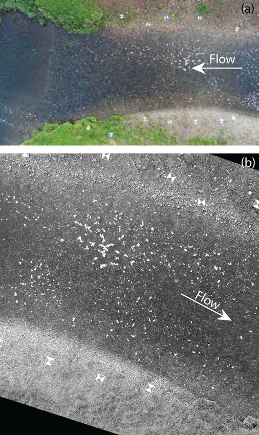
1546                                                        M. T. Perks et al.: Harmonisation of image velocimetry techniques

1   Introduction                                                   techniques have chosen to develop their own specific pro-
                                                                   cessing capabilities, leading to the development of a range
                                                                   of both open-source and proprietary software for image pre-
When designing hydrological monitoring networks or ac-             processing and velocimetry analysis (Table A1). Whilst this
quiring opportunistic measurements for determining open-           has led to a breadth of options for researchers conducting im-
channel flow, the optimum choice of apparatus is likely to be      age velocimetry analysis, inter-comparisons of their efficacy
a compromise between the data requirements, resource avail-        under a range of environmental settings and flow regimes is
ability, and the hydro-geomorphic characteristics of the site      currently lacking (Pearce et al., 2020). Therefore, there is
(Mishra and Coulibaly, 2009). Generally, hydro-geomorphic          an urgent need to comprehensively understand and appreci-
factors will include: channel width and depth, the range of        ate limitations of the differing image velocimetry approaches
flow velocities, presence of secondary circulation, and cross      that are available to the scientific community.
section stability. Each field measurement technique will have         Here, we present a range of datasets that have been com-
a designed range of optimum operating conditions under             piled from across seven countries in order to facilitate these
which robust flow measurements should be expected (e.g.            inter-comparison studies (Fig. 1, Perks et al., 2020). These
ISO 24578:2012). However, under conditions beyond their            data have been independently produced for the primarily pur-
designed operating range, greater levels of uncertainty will       poses of (i) enhancing our understanding of open-channel
ensue. This may therefore preclude certain approaches for          flows in diverse flow regimes and (ii) testing specific im-
deployment under very shallow or flood flow conditions, for        age velocimetry techniques. These datasets have been ac-
example. Logistical and practical constraints may also limit       quired across a range of hydro-geomorphic settings, using a
the deployment of apparatus. For example, techniques that          diverse range of cameras, encoding software, and controller
require the device to be in contact with the water during op-      units. Image sequences have then been subjected to a range
eration may not be feasible for health and safety reasons dur-     of differing image pre-processing steps using a range of im-
ing periods of high flow or due to staff availability (Harpold     age processing software. The compilation of these diverse
et al., 2006). As a result of some of these challenges, the po-    datasets offers the research community a resource for ad-
tential for implementing alternative, non-contact approaches       dressing key challenges that have been identified in the use
has been recently explored. Within this field of research, im-     of image velocimetry algorithms. These include (but are not
age velocimetry has emerged as an exciting new approach for        limited to) the potential for the characteristics of the seeding
determining a key hydrological characteristic, namely flow         material (e.g. particle density) to affect the resultant velocity
velocity.                                                          estimates (Dal Sasso et al., 2018; Pizarro et al., 2020), the
   Image velocimetry involves the application of cross-            impact of UAS movement on velocity measurements (Lewis
correlation or computer vision techniques on a series of con-      and Rhoads, 2018), and the testing of different image sta-
secutive images (or extracted video frames) to generate vec-       bilisation approaches to address this. Additional assessments
tors of water velocities across a field-of-view. It was origi-     may concern the role of image pre-processing (e.g. back-
nally developed for use in highly controlled laboratory set-       ground suppression; Thielicke and Stamhuis, 2014) and the
tings. However, since its original conception, its applica-        role of pixel resolution and video length on errors under dif-
tion has expanded from use in the laboratory (e.g. Dudderar        fering flow conditions (Tauro et al., 2018b).
and Simpkins, 1977; Adrian, 1984; Pickering and Halliwell,
1984) to include a wide variety of experimental conditions.
Most notably it has been deployed outside of the controlled        2   Experimental design
environment of the laboratory and into the domain of the
field scientist (e.g. Fujita et al., 1998). It is now applied in   Given the range of image velocimetry techniques that have
complex environments including situations where lighting is        been developed in recent years, benchmarking datasets cov-
not controlled, the camera platform may be mobile (e.g. on         ering a range of hydro-geomorphic conditions and acquisi-
unmanned aerial systems, UASs), images may be acquired             tion platforms are required in order to test the accuracy and
oblique to the direction of flow, and at an angle that changes     precision of each algorithm for the determination of one-
over time (e.g. Detert and Weitbrecht, 2015; Tauro et al.,         and two-dimensional surface velocities. The examples that
2016b; Perks et al., 2016).                                        we describe in this section have been acquired by a range of
   This technique is also becoming increasingly popular with       platforms, including UAS and fixed and handheld cameras.
the wider hydrological community (Tauro et al., 2018a), and        The geographical characteristics of the sites also widely var-
this has been aided by two key factors. The first of which is      ied. Catchment areas span 20–17 460 km2 , captured channel
the development of platforms and hardware that enable high-        widths range from 5–59 m, minimum flow depth is 0.10 m
definition images and videos to be captured precisely, stored,     with a maximum of over 7 m, and mean flow velocities range
and transferred to locations where image processing can oc-        from 0.13 to over 6 m s−1 . Where possible, reference data
cur. Secondly, many researchers utilising image velocimetry        generated by established and widely accepted approaches

Earth Syst. Sci. Data, 12, 1545–1559, 2020                                         https://doi.org/10.5194/essd-12-1545-2020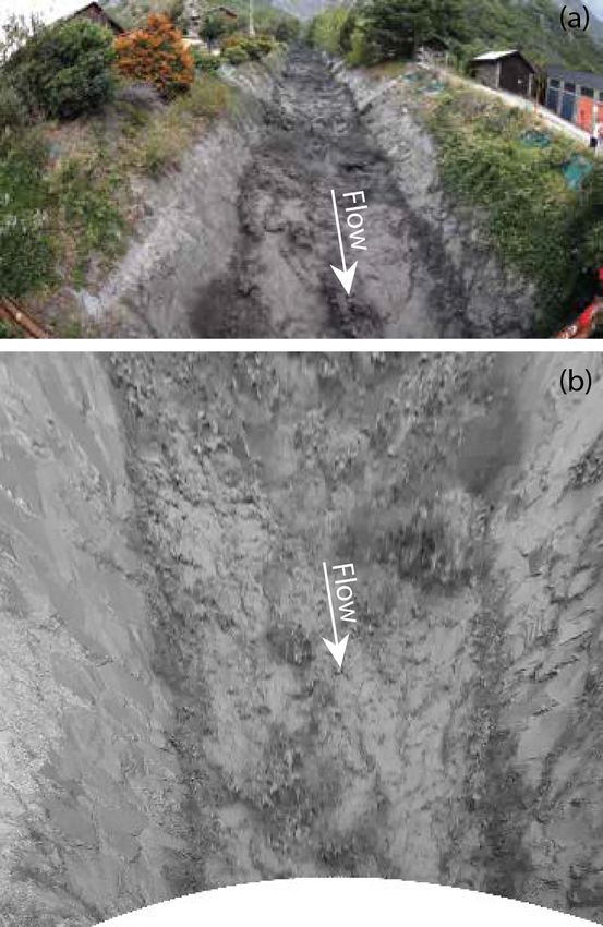
M. T. Perks et al.: Harmonisation of image velocimetry techniques                                                                 1547

                                                                       era CMOS sensor. This was used to collect nadiral footage,
                                                                       with the camera’s y axis orthogonal to the direction of flow.
                                                                       Video was collected by the UAS for 4 min 18 s whilst hov-
                                                                       ering at an elevation of approximately 20 m over the field
                                                                       of interest (Fig. 2a). Footage was recorded at a pixel reso-
                                                                       lution of 1920 × 1080 and frame rate of 30 Hz. The second
                                                                       approach consisted of a GoPro Hero 4 mounted at an oblique
                                                                       angle on a stationary telescopic pole at a height of approx-
                                                                       imately 2 m above the water surface. Video footage was si-
                                                                       multaneously collected for 5 min 37 s at a pixel resolution of
                                                                       1920 × 1080 and frame rate of 30 Hz. During the period of
                                                                       recording, sequences consisting of both unseeded flow and
                                                                       artificially seeded flow are visible. For the seeded element,
                                                                       cornstarch Ecofoam chips were added to the water surface
                                                                       immediately upstream of the area of interest. These tracers
                                                                       are clearly visible in the footage and are distributed evenly
                                                                       in the cross section. Seeding was carried out to enhance the
                                                                       availability of traceable features in the low-flow conditions.
                                                                          From the recordings, datasets each consisting of 99 con-
Figure 1. Locations of the monitoring sites from which data are        secutive images (sampled at a frame rate of 5 Hz and con-
presented: (1) River Arrow, UK; (2) River Thalhofen, Germany;          verted to greyscale intensity) were extracted from both the
(3) Murg River, Switzerland; (4) Alpine river, Austria; (5) River
                                                                       UAS and GoPro footage under both seeded and unseeded
Brenta, Italy; (6) La Morge, France; (7) St. Julien torrent, France;
                                                                       conditions. As a result of camera movement for both the
(8) River La Vence, France; (9) River Tiber, Italy; (10) River
Bradano, Italy; (11) River Noce, Italy. Not shown are the fol-         UAS and GoPro footage, image sequence stabilisation was
lowing rivers in North America: (12) Castor River, Canada, and         carried out using Fudaa-LSPIV (Table A1). In order to en-
(13) Salmon River, Canada. Map spatial reference: ETRS (1989).         able the conversion of pixel units to metric units, a total of 10
                                                                       ground control points (GCPs), which were visible throughout
                                                                       the duration of the video, were distributed across both banks
(e.g. current meter and acoustic Doppler current profiler,             (Fig. 2a). These GCPs were surveyed and their positions
ADCP) have been collected simultaneously or at the same                utilised for image orthorectification using Fudaa-LSPIV (Ta-
river stage as the images are acquired. The details pertaining         ble A1). Subsequently, the orthorectified images have a scal-
to the hydrological conditions of deployment, configuration            ing of 0.0174 m px−1 (Fig. 2b).
of the camera setup, pre-processing of imagery, and (where                Reference data were obtained through the deployment of
relevant) details of published results from these datasets are         a Valeport 801 electromagnetic current meter. Measurements
presented in the following sections and summarised in Ta-              were made for a period of 30 s just below the water sur-
ble A2.                                                                face, with the time-averaged value being reported. Measure-
                                                                       ments were obtained for five cross sections spaced approx-
2.1   River Arrow, UK
                                                                       imately 1.5–2 m apart, within which 9–10 individual mea-
                                                                       surements were obtained with a spacing of 0.5 m between
On 1 November 2017, a field experiment was undertaken on               each. The location of each measurement is provided in pixel
the River Arrow in Warwickshire, UK, to ascertain the ac-              units based on the stabilised and orthorectified imagery of the
curacy of two differing image velocimetry approaches. The              UAS and GoPro.
location of this experiment was in the mid-reaches of the
catchment, with a contributing area of 94 km2 . This is a sta-         2.2   River Thalhofen, Germany
ble, meandering section of the river with an approximate
width of 5 m. During the experiment, mean depth and ve-                On 27 July 2017, a Vivotek IB836BA-HT network surveil-
locity were 0.22 m and 0.42 m s−1 , respectively, and water            lance camera was utilised to capture footage for image ve-
turbidity was minimal, with the gravel bed being clearly vis-          locimetry analysis on the River Thalhofen in Germany. At the
ible in the footage.                                                   time of deployment, the river width was approximately 28 m,
   The two deployments differed, as both fixed (bankside               the river stage was 1.45 m, and ADCP derived discharge and
pole-mounted) and mobile (UAS) imaging systems were                    mean velocity were 52.52 m3 s−1 and 1.7 m s−1 , respectively.
used. Footage acquired from these two systems was captured             The camera was fixed in location, with the camera lens at an
concurrently, permitting direct comparisons to be made be-             approximate angle of 25◦ from nadir and the image y axis
tween the two. The mobile imaging system consisted of a                approximately 5◦ from being perpendicular to the direction
DJI Phantom 4 Pro UAS equipped with a 1 in. (2.54 cm) cam-             of flow. Images were collected for a duration of 2 s at a reso-

https://doi.org/10.5194/essd-12-1545-2020                                             Earth Syst. Sci. Data, 12, 1545–1559, 2020
1548 M. T. Perks et al.: Harmonisation of image velocimetry techniques
2.3 Murg River, Switzerland
On 6 April 2016, aerial surveys were undertaken in order
to acquire imagery for determining the bathymetry and sur-
face velocity and to subsequently derive the flow discharge
of the Murg River, Switzerland (Detert et al., 2017). The
experiment took place in the middle reaches of the catch-
ment, with a contributing area of 212 km2 . The experimental
reach was a stable, straight section totalling 75 m in length,
along which, the water depth was approximately 0.35 m and
channel width was 12 m. The discharge at the time of survey
was 2.76 m3 s−1 . For the aerial survey a DJI Phantom FC40
was deployed at a stable altitude of 30 m to track the move-
ment of artificial tracers throughout the reach. The UAS was
equipped with a GoPro Hero3+ Black Edition 4K camera,
which is capable of capturing a large spatial footprint whilst
deployed at a relatively low altitude. However, this also gen-
erates a considerable barrel distortion effect that must be
overcome during image processing. This system was used
to collect nadiral footage, with the camera’s y axis perpen-
dicular to the flow direction. Video footage was acquired for
a period of 2 min 11 s at a pixel resolution of 4096 × 2160
and a frame rate of 12 Hz. During image acquisition, the wa-
ter was clear, with the channel bed visible in places. These
conditions resulted in a lack of naturally occurring features
visible on the water surface that could be used to determine
surface velocity. Therefore, throughout the duration of the
experiment, spruce woodchips were applied to the water sur-
face from a bridge at the upper extent of the monitored reach.
This artificial seeding produced a dense, vivid, and homoge-
neously distributed pattern of features, the displacement rate
Figure 2. (a) Footage acquired by the Phantom 4 UAS over the of which is considered to equate to the surface velocity. From
River Arrow and (b) following orthorectification and greyscale con- the video recordings, 1000 images were orthorectified using
version. The Ecofoam chips and ground control points are clearly Photoscan (Agisoft). This was achieved through the input of
visible in both images. The direction of flow is indicated by the ar- geographical coordinates relating to 14 GCPs that were vis-
rows. ible at varying times throughout image sequence. This ap-
proach is discussed further in Detert et al. (2017). The sub-
sequent orthorectified images are presented at a time step
lution of 1280 × 800 px and frame rate of 30 Hz. Despite the of 0.083 s, and the raster pixel scale was consistently set at
presence of highly turbid water, which can diminish contrast 64 px m−1 , equivalent to pixel dimensions of 0.0156 m in the
across the water surface, the presence of highly visible tur- x and y axes. Metadata describing the scale of the image per
bulent structures advecting downstream offers the potential pixel and the [x, y] coordinate of the upper-left pixel of each
for the extraction of surface velocity information from these image are provided in the corresponding .jgw file.
images. Image pre-processing consisted of orthorectification Reference data were acquired through the deployment of
(using Photrack software; see Table A1) and colour conver- a Teledyne RDI StreamPro ADCP across a single transect in
sion to greyscale. A total of 56 consecutive images that have the upper reaches of the studied site. ADCP data were ac-
been subjected to these processing steps are presented here quired with a bin depth of 0.02 m, with the uppermost mea-
at their original frame rate of 30 Hz. The pixel dimensions of surement occurring at a distance of 0.14 m below the water
the processed imagery are 0.01 m in the x and y axes. surface. A total of 85 measurements of the velocity magni-
Reference data were acquired by means of a Teledyne tude are presented with an average spacing of 0.14 m.
RiverPro ADCP and consist of a single transect consisting
of 280 measurements along the cross section with an aver- 2.4 Alpine river, Austria
age spacing of 0.09 m. ADCP data were acquired with a bin
depth of 0.06 m, with the uppermost measurement occurring On 7 August 2019, aerial surveys were undertaken in order
at a distance of 0.22 m below the water surface. to assess the flow conditions at the turbine outlet of a hy-
Earth Syst. Sci. Data, 12, 1545–1559, 2020 https://doi.org/10.5194/essd-12-1545-2020M. T. Perks et al.: Harmonisation of image velocimetry techniques 1549
dropower dam, the entrance of a fish passage, and the area 2.5 River Brenta, Italy
immediately downstream of these features (Strelnikova et al.,
2020). The Alpine river (epithet), is located in Austria, and Two distinct experimental approaches have been adopted to
can be characterised as having a nivo-glacial hydrological generate datasets that describe flows in the 252 km2 catch-
regime, with a drainage area of 1057 km2 and a mean flow ment of the River Brenta. The first involved the temporary
discharge of over 32 m3 s−1 . At the time of data acquisition installation of a GoPro Hero 4 Black Edition camera attached
the water turbidity was minimal, such that a rocky brown– to a telescopic apparatus on the downstream side of a bridge
green riverbed was distinctly visible. Several rocky islands (Tauro et al., 2014). During this deployment, river flow was
and multiple boulders were located in the middle of the low, with an observed mean velocity of 0.38 m s−1 . To com-
river section of interest. The river section contained turbu- pensate for the lack of naturally occurring features on the
lent spots and was characterised by heterogeneous flow con- water surface, woodchips were manually added to the river
ditions, with partially opposite flow directions and velocities upstream of the monitoring site, resulting in continuous and
ranging from 0 to approximately 2 m s−1 . Within the study relatively homogeneous coverage for the 20 s duration of the
area, the river was up to 35 m wide, with depths ranging from image sequences. The camera’s field of view was 9.5×5.3 m2
0.10 to 2 m. and was configured to collect 1920 × 1080 HD videos at a
Footage of the area was recorded using a DJI Mavic Pro frame rate of 50 Hz. Distortion of the images as a result of
UAS in a hovering mode from an altitude of 50 m at a frame the fisheye lens was removed using the open-source software
rate of 25 Hz, with a resolution of 3840 × 2160 px. The built- GoPro Studio. No subsequent orthorectification of the im-
in camera of the UAS was directed at nadir. During data ac- ages was required due to the camera apparatus being installed
quisition, the flow was artificially seeded with biodegradable perpendicular to the water surface. The pixel dimensions of
cornstarch Ecofoam. Individual Ecofoam pieces had a cylin- the processed imagery were 0.005 m in the x and y axes.
drical shape that was 1.5–2 cm in diameter and 4.5–6 cm in This could be established either through the projection of two
length. Tracers were added into the flow from seven loca- lasers at a fixed and known distance apart to the surface of the
tions: over the entrance into the fish ladder, over the turbine river or through identification of a fixed and known object in
outlet, from the islands, and from both banks. The duration the field of view. In terms of pre-processing of the imagery,
of an acquired video was 5 min. From this video, a dataset of an area of 552 × 375 pixels in the bottom right corner of the
897 images was extracted at 12.5 Hz and stabilised using a images was masked with a black patch. This was to elimi-
custom MATLAB script. A subset of the footage was used in nate noise generated by mobile vegetation within the frame.
a study described by Strelnikova et al. (2020). Original RGB images were converted to greyscale intensity
For image calibration, 11 GCPs visible in each of the ex- by eliminating hue and saturation information and retaining
tracted frames were used. A total of 7 GCPs were distributed the luminance. To emphasise lighter particles against a dark
across both river banks, and 4 GCPs were located on the is- background, images were gamma corrected to darken mid-
lands. The GCPs were surveyed with the use of a differential tones. A total of 12 separate image sequences lasting 20 s,
GPS with an accuracy of ±3 cm. The pixel dimensions of the sub-sampled at 25 Hz, and consisting of 500 frames each are
calibrated imagery are 0.021 m in the x and y axes. presented here.
An OTT C31 propeller current meter was used to per- The second experimental approach involved the temporary
form reference measurements just below the water surface deployment of a FLIR Systems AB ThermaCAM SC500.
at 23 locations. During reference data acquisition the pro- This was suspended from a mobile supporting structure on
peller axis aligned with the direction of the flow. The du- the downstream side of a bridge at approximately 7 m above
ration of measurement at each point was 1 min. The distri- the water surface (Tauro and Grimaldi, 2017). As opposed
bution of reference measurements (Fig. 3) was selected in to capturing images in the usual red, green, and blue bands,
a way that described all important components of the het- this camera is sensitive to thermal infrared radiation, gen-
erogeneous flow: the flow from the fish ladder entrance, the erating a monochrome image with values proportionate to
dominant flow from the turbine outlet, areas around the main the thermal properties of the objects within the field of view.
flow curve, and two branches of the main flow after its split. The application of this approach for image velocimetry re-
Flow directions were determined using a compass with 10◦ quires a distinct thermal signal to be present from either nat-
precision in degrees from north. The footage was recorded in ural (e.g. tributary confluences with water of differing ther-
a way that north corresponded to 97◦ measured in the clock- mal properties) or artificial sources. In this instance, an arti-
wise direction from the image top (see the north arrow in ficial thermal signal was introduced in the form of ice dices.
the bottom right corner of Fig. 3). The locations of reference These were deployed upstream of the bridge and were ob-
measurements were determined with the use of a differential served transiting across the field of view as a result of their
GPS with an accuracy of ±3 cm. The accuracy of the pro- thermal properties being sufficiently different to those of the
peller current meter was ±2 %. water surface. Despite the image resolution being a modest
318 × 197 pixels with a frame rate of 5 Hz, this was still suf-
ficient to enable movement of the ice dices to be tracked.
https://doi.org/10.5194/essd-12-1545-2020 Earth Syst. Sci. Data, 12, 1545–1559, 20201550 M. T. Perks et al.: Harmonisation of image velocimetry techniques
Figure 3. A snapshot from footage acquired proximal to a fish ladder on the Alpine river. The distribution of reference measurements with
corresponding velocity magnitudes (m s−1 ) are shown. The dominant direction of flow is indicated by the arrow.
Geometric calibration of the images was achieved by iden- logue Panasonic WV-CP500 camera with a focal length of
tifying features of known dimensions within the video se- 4 mm. This camera was mounted at an elevated position on
quence (i.e. three wooden sticks). The pixel dimensions of a 3 m pole on the right bank of the channel, oriented in an
the processed imagery are 0.009 m in the x and y axes. Here upstream direction. Images were collected with an effective
we present an image sequence consisting of 80 consecutive pixel resolution of 640 × 480 at a frame rate of 5 Hz for a
frames captured over 16 s. duration of 10 s, resulting in the generation of 48 images.
Reference validation data are available in the form of ve- On this occasion, manual seeding of corn chips took place
locity measurements taken at just 3 cm below the water sur- immediately upstream of the camera’s field-of-view to en-
face at four locations along the stream cross section using hance the occurrence of features for tracking purposes. This
an OTT Hydromet C2 current meter. At each measurement is typically required where natural seeding is inhomogeneous
location 12 replicate measurements were made (Tauro et al., or completely lacking. Following acquisition of the footage,
2017). images were converted to greyscale and orthorectified using
Fudaa-LSPIV to generate images in which 1 pixel represents
2.6 La Morge River, France a real-world distance of 0.01 m.
Reference data were acquired 5 m downstream of the
Within Electricité De France’s (EDF) network of over video acquisition location so as to not interfere with the
300 hydrological monitoring stations for the optimal man- recorded footage. Therefore, comparisons between measured
agement of water resources, image-based velocimetry ap- velocities using image velocimetry and traditional gauging
proaches have recently been adopted. This approach has methods in the same cross section is not possible. How-
been specifically adopted with the aim of reducing uncer- ever, a comparison of the computed river discharge from
tainty under high-flow conditions (Hauet, 2016). These con- the differing methods is possible. At the upstream location
ditions can develop rapidly, particularly during the summer (the camera-monitored reach), water depth measurements are
months as a result of convective storms, posing difficulties available for two transects separated by approximately 6 m
for traditional monitoring approaches. However, this setup with an average spacing between points of 0.25 m. Through
may also be applied to capture images for the determination the application of image velocimetry techniques, water depth
of surface velocity under more quiescent conditions. Here, measurements, and an appropriate value relating the sur-
we present images captured on 13 January 2015 in the small face velocity to the depth-averaged velocity (estimated to be
(46 km2 ), urban catchment of La Morge with a mean altitude 0.85), river discharge can be computed. At 5 m downstream
of 270 m. Flow conditions were typical, with a cross section of the camera, velocity data were acquired through the use of
width of 7.2 m, mean depth of 0.41 m, and mean velocity of a mechanical current meter, with measurements taken at 0.2,
0.39 m s−1 . The imaging system used consisted of an ana-
Earth Syst. Sci. Data, 12, 1545–1559, 2020 https://doi.org/10.5194/essd-12-1545-2020M. T. Perks et al.: Harmonisation of image velocimetry techniques 1551
0.6, and 0.8 of the river depth. A total of 15 measurements
were made along the cross section at intervals of 0.5 m. De-
tailed measurements are provided along with the river dis-
charge computed from these observations. Given the small
distance of 5 m between the location of the recorded video
footage and in-stream measurements and the lack of gains or
losses within the reach, river discharge would be the same
value at both locations.
2.7 St. Julien torrent, France
A high-magnitude flash flood occurred in the St. Julien tor-
rent system during August 2011. This was captured by a
local storm chaser using a Canon EOS 5D mark II cam-
era with a 16 mm fisheye Zenitar lens. Like many headwater
systems across Europe, no hydrological monitoring networks
are present in this torrent system. Therefore, this footage pro-
vides a rare insight into the hydraulic processes occurring
during a flash flood in a steep, small (20 km2 ) torrent system
where mean flow velocities are approximately 6 m s−1 . The
footage itself was recorded at a resolution of 1920 × 1080 px
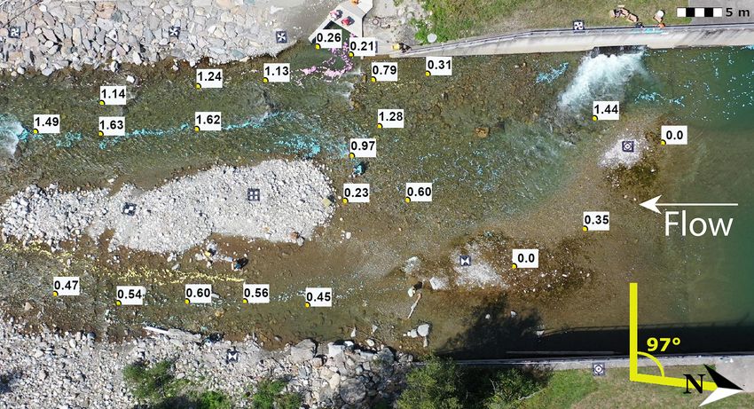
at a frame rate of 25 Hz (Fig. 4a). The footage was not
filmed from a fixed location; therefore, complications in-
volving camera movement and orthorectification had to be
overcome. These steps are explained in detail in Le Bour-
sicaud et al. (2016). Following correction for these factors,
a sequence of 51 consecutive and geometrically stable im-
ages are produced (Fig. 4b). Each pixel width represents a
metric scale of 0.03 m. Despite the lack of detailed reference Figure 4. (a) Original footage of a flash flood in the St. Julien tor-
velocity measurements for this case study, researchers inter- rent acquired by a storm chaser equipped with Canon EOS 5D mark
ested in reconstructing flash flood processes may find it valu- II camera. (b) Orthorectified and geometrically stable image with
the field of view clipped to the lower 50 % of the image. The direc-
able for understanding how the range of available methods
tion of flow is indicated by the arrows.
perform relative to each other, given that image velocime-
try techniques perhaps offer the best opportunity to estimate
flows under these extreme conditions.
at their original frame rate of 30 Hz. The pixel dimensions of
the processed imagery are 0.008 m in the x and y axes.
2.8 River La Vence, France Reference data were acquired by means of a HydroProfiler
M-pro ADCP and consist of a single transect consisting of
On 8 May 2019, a Samsung Galaxy S7 was utilised to cap- eight measurements with an average spacing of 0.7 m. ADCP
ture footage for image velocimetry analysis on the River La data were acquired with a bin depth of 0.003 m with the up-
Vence, a 63.75 km2 catchment in France. At the time of de- permost measurement occurring at a distance of 0.101 m be-
ployment, the river width was approximately 6.3 m, with a low the water surface.
river stage of 0.44 m. A discharge of 1.15 m3 s−1 and mean
velocity of 0.65 m s−1 were observed. The camera was fixed 2.9 River Tiber, Italy
in location, with the camera lens angled at approximately 31◦
from nadir and the image x axis at approximately perpen- A permanent gauge station on the River Tiber, Italy, was in-
dicular to the direction of flow. Images were collected for a stalled to test the feasibility for automated image velocime-
duration of 5 s at a resolution of 1920 × 1080 px and frame try methods to quantify the flow rates of a major European
rate of 30 Hz. The presence of visible turbulent structures ad- river with a catchment area of 17 460 km2 . This deployment
vecting downstream offer the potential for the extraction of involves the use of a Mobotix FlexMount S15 IP camera
surface velocity information from this footage. Image pre- attached to the underside of Ponte del Foro Italico, in the
processing consisted of orthorectification, and colour conver- city of Rome (Tauro et al., 2016a). The wide-angle lens
sion to greyscale. A total of 150 consecutive images that have on the SP15 camera introduces distortion into the images,
been subjected to these processing steps are presented here which was subsequently removed using the Adobe Photo-
https://doi.org/10.5194/essd-12-1545-2020 Earth Syst. Sci. Data, 12, 1545–1559, 20201552 M. T. Perks et al.: Harmonisation of image velocimetry techniques
shop Lens correction filter. In a similar setup to the first of the were subsequently undertaken. This included conversion of
River Brenta approaches, this camera is positioned orthog- the greyscale images to black and white, and contrast correc-
onal to the water surface, thereby circumventing the need tion in order to more prominently highlight the artificial trac-
for orthorectification of the generated images. Transforma- ers on the water surface. A total of 600 images that have been
tion of the camera pixels (px) to metric units (m) was again subjected to these processing steps are available at their orig-
achieved by firing lasers of a known distance apart at the inal resolution and frame rate. An additional processing step
water surface. The image can be scaled to metric distances involved the stabilisation of the image sequence to minimise
given: 1 px = 0.016 m. The camera itself generated videos apparent movement of the platform. Transformation of the
with a resolution of 2048 × 768 px. However these were sub- images from pixel units to metric distance can be achieved
sampled to 865 × 530 px at a frame rate of ≈ 6.95 Hz during using the following function: 1 px = 0.009 m. Validation data
pre-possessing. The data specifically presented here consists in the form of surface velocities was obtained at seven points
of 410 consecutive frames collected over a 60 s period dur- in the cross section, at 1 m intervals using a Seba F1 current
ing a moderate flood event in February 2015. At the time of flowmeter. The locations of these measurements are provided
acquisition, the river stage was 7.23 m and the average sur- in pixels relative to the first frame of the stabilised image se-
face velocity (measured by a RVM20 speed surface velocity quence.
radar) was 2.33 m s−1 (Tauro et al., 2017). Whilst only a sin-
gle reference velocity value is available, this measurement is 2.11 River Noce, Italy
representative of the surface velocities within a surrounding
area of approximately 3×3 m2 . The approximate spatial foot- On 26 July 2017, in the middle reaches of the 413 km2 ,
print of the surface velocity radar measurement is provided single-thread, River Noce, a DJI Phantom 3 Pro UAS Sony
in pixel units. EXMOR 1/2.3 in. (1.10 cm) CMOS sensor was deployed to
capture footage for image velocimetry analysis (Dal Sasso
et al., 2018). At the time of deployment, water levels were
2.10 River Bradano, Italy low, with an observed discharge of 1.70 m3 s−1 and mean
On 14 October 2016, an experiment was undertaken in or- velocity of 0.43 m s−1 . Turbidity was also minimal, result-
der to explore the optimal setup for the acquisition of surface ing in the gravel bed being distinctly visible in the footage.
flow velocity measurements using an UAS (Dal Sasso et al., The camera was oriented with its x axis perpendicular to the
2018). The experiment took place in the valley portion of the water surface, enabling the 14.6 m wide channel to be fully
Bradano River, located in the Basilicata region of Italy. This observed (Fig. 5a). Images were collected for a duration of
large alluvial river has a catchment area of 2581 km2 and is 1 min 48 s at a resolution of 3840 × 2160 px and frame rate
characterised by low gradient (0.1 %) and low relative sub- of 24 Hz. The clear water and bright sunlight results in non-
mergence (Dal Sasso et al., 2018). At the time of the exper- homogeneous illumination of the water surface. This is par-
iment, the cross section width was 11.4 m, with a maximum ticularly apparent in the lower-left quarter of the video frame.
depth of 0.80 m. The average surface velocity was 0.75 m s−1 Naturally occurring tracers are also largely absent, making
and total discharge was 3.97 m3 s−1 . During the experiment, these challenging conditions for the application of image ve-
a DJI Phantom 3 Pro UAS equipped with a Sony EXMOR locimetry techniques. To offset these issues, woodchips were
1/2.3 in. (1.10 cm) CMOS camera sensor was deployed. introduced upstream of the monitoring location. These fea-
The UAS hovered over the centre of the River Bradano tures were visibly brighter than the background, enabling
with a nadir camera positioned perpendicular to the direc- their transition to be detected optically. Image processing
tion of flow. An area of 17.0 × 9.6 m2 was imaged, includ- consisted of contrast stretching and conversion of greyscale
ing the entire cross section of interest (with a width of ap- images to black and white in order to enhance the visibility of
proximately 11.4 m). Video footage was captured for a dura- the artificial tracers against the background (Fig. 5b). A total
tion of 1 min 43 s at a pixel resolution of 1920 × 1080, and of 70 consecutive images that have been subjected to these
a frame rate of 24 Hz. Due to the high turbidity of the flow, processing steps are presented here at a downscaled resolu-
there is a weak natural contrast across the image which di- tion of 1920 × 1080 px and frame rate of 12 Hz. Following
minishes the number of naturally occurring visible tracers. sub-sampling, each pixel in the image represents a distance
Therefore, throughout the duration of the footage, operatives of 0.009 m in metric units. Validation data in the form of sur-
manually introduced charcoal to the water surface immedi- face velocities were obtained at 13 locations at 1 m intervals
ately upstream of the monitoring site. The colour of these along the cross section using a Seba F1 current flowmeter.
particles was sufficiently distinct from the background to en- The locations for each of these measurements is provided in
able their displacement to be optically tracked. However, the pixel units.
distribution of these tracers is generally limited to the cen-
tral portion of the flow, which may limit the availability of
traceable features towards the channel boundaries. Follow-
ing collection of the footage, a number of processing steps
Earth Syst. Sci. Data, 12, 1545–1559, 2020 https://doi.org/10.5194/essd-12-1545-2020M. T. Perks et al.: Harmonisation of image velocimetry techniques 1553
at varying heights across both sides of the channel, and the
distances and horizontal and vertical angles between points
were surveyed using a tripod-mounted Leica S910. This en-
abled a local coordinate system to be developed relative to a
local benchmark. In the resultant imagery each image pixel
represents a distance of 0.01 m in metric units.
Reference data were acquired through the deployment of
a Teledyne RDI StreamPro ADCP, with four transects be-
ing completed across a single cross section. ADCP data were
acquired with a bin depth of 0.05 m with the uppermost mea-
surement occurring at a distance of 0.17 m below the water
surface. Between 149 and 219 velocity magnitude measure-
ments are reported for each transect, with an average spacing
between measurements of 0.12–0.18 m. The location of each
velocity magnitude measurement is reported in pixel units
based on the orthorectified imagery.
The second video set obtained at Castor River was ac-
quired on 9 July 2019 and consists of a single 27 s video.
This was acquired from the left bank using a ACTI A31
IP camera, mounted at an oblique angle of 54◦ from nadir.
Video footage was recorded at a resolution of 1920×1080 px
and frame rate of 30 Hz. At the time of acquisition, river
levels were low, with a reported stage of 3.128 m. At this
time, the river was 21 m wide with a mean and maximum
Figure 5. (a) Greyscale footage acquired by the Phantom 3 UAS
depth of 0.45 and 0.62 m, respectively. Observed discharge
over the River Noce and (b) the same image following contrast
stretching. The direction of flow is indicated by the arrows.
was 0.93 m3 s−1 with a mean velocity of 0.13 m s−1 . No im-
age stabilisation was performed on the image sequence and
the imagery was orthorectified using KLT-IV and the same
2.12 Castor River, Canada ground control points as the previous set of videos. In the
resultant imagery each image pixel represents a distance of
Here we present footage acquired from the middle reaches 0.01 m in metric units. Reference data were acquired using
of the Castor River in Ontario, Canada (45.26194◦ latitude, a FlowTracker2 handheld acoustic Doppler velocimeter. Ve-
−75.34444◦ longitude). At this location, the channel is a locity measurements were made at four locations along a sin-
stable, single-thread, meandering river with a catchment- gle cross section and at percentage depths of 0 (i.e. water
contributing area of 439 km2 . Footage was acquired on two surface), 20 %, 40 %, 60 %, 80 %, and 100 %. The x and y
separate occasions, consisting of very different flow condi- velocity components are reported along with the mean veloc-
tions. ity. The location of each velocity measurement is reported in
The first set of videos were acquired on 10 April 2019 us- pixel units based on the orthorectified imagery.
ing a Hikvision DS-2CD2T42WD-I5 4 mm IP camera. This
was mounted on the left bank at an oblique angle of 57◦ from 2.13 Salmon River, Canada
nadir. Video footage was captured consisting of three 30 s
videos at a resolution of 2688 × 1520 px and frame rate of On 4 June 2019, a DJI Phantom 4 Pro was used to acquire
20 Hz. The first 2–3 s of each recording have been removed footage over the Salmon River in British Columbia, Canada
from the submission as these frames experienced compres- (50.312222◦ latitude, −125.907500◦ longitude). Footage
sion and frame rate issues. However, the remainder of the was acquired immediately downstream of the confluence be-
video is unaffected. The videos were captured over a duration tween the Salmon River and the smaller White River. Here,
of approximately 4.5 h and over this time the river stage was the catchment contributing area is 1210 km2 , and a 59 m wide
stable, varying between 3.772 m at 11:25, 3.769 m at 13:45, single-thread channel is present. At the time of image acqui-
and 3.77 m at 15:55 (local time). Under these moderate flow sition, river levels were low, with an average depth of 0.65 m,
conditions, mean velocity was observed to be 1.26 m s−1 , a reported discharge of 22.9 m3 s−1 , and mean velocity of
with mean and maximum depths of 0.80 and 1.19 m, respec- 0.65 m s−1 . A 1 min video was collected with a view angle of
tively, within the 27 m wide river. No image stabilisation was approximately nadir whilst hovering at an elevation of 102 m
performed on the image sequence and the imagery was or- over the field of interest. The footage was acquired at a res-
thorectified using KLT-IV (Perks et al., 2020) and the use of olution of 1920 × 1080 px and a frame rate of 24 Hz. Present
12 ground control points. These control points were placed within the field of view are four ground control points located
https://doi.org/10.5194/essd-12-1545-2020 Earth Syst. Sci. Data, 12, 1545–1559, 20201554 M. T. Perks et al.: Harmonisation of image velocimetry techniques
on both sides of the channel. The straight-line distances be- This unique dataset represents the first step in creation of
tween each of the ground control points were measured and a community database for image velocimetry benchmarking
a local coordinate system developed following the principles studies. It offers the hydrological community the opportunity
of trilateration. A two-stage processing method was adopted to assess the accuracy of existing approaches under a range of
to generate imagery suitable for velocimetry analysis. This conditions. Key comparisons may be made surrounding the
consisted of (i) image stabilisation and (ii) orthorectifica- relative impact of the seeding characteristics (e.g. River Ar-
tion. These were performed using the built-in functionality of row, Murg River), the type of sensor used (e.g. River Brenta),
KLT-IV (Table A1). Following processing, each image pixel the potential for background noise, e.g. glare, visible river
represents a distance of 0.01 m in metric units. Reference bed, to be filtered (e.g. Salmon River), and the impacts of
velocity data were acquired using a FlowTracker handheld stabilisation on velocity outputs (e.g. River Bradano, Alpine
acoustic Doppler velocimeter and this consists of measure- river).
ments at 26 locations along a single cross section at intervals The generation of similar datasets of images is widely used
of approximately 3 m. These measurements were obtained at to evaluate the effectiveness and accuracy of algorithms in
60 % of the water depth, and the mean velocity is reported. related fields such as fluid mechanics (e.g. Okamoto et al.,
The location of each velocity measurement is reported in 2000), and we envisage such a dataset for large-scale flu-
pixel units based on the orthorectified imagery. vial environments will encourage further scientific assess-
ment and development of image velocimetry approaches.
3 Data availability Though the diversity of experimental settings and data
formats included in this dataset may limit the inter-
Datasets presented in this manuscript can be comparability of experiments, this dataset is well suited for
readily downloaded from the following website: comparison of different algorithms within the framework of
https://doi.org/10.4121/uuid:014d56f7-06dd-49ad-a48c- one selected study. An advantage of the dataset is that it is
2282ab10428e. Data includes the footage and imagery representative of the multitude of possible experimental set-
required for image velocimetry analysis, plus validation data tings. Techniques tested and tailored with the help of such a
for 12 of the 13 case studies presented. Please contact the diverse dataset are expected to be more robust, and their limi-
corresponding author if further details are required (Perks tations are expected to be easier to identify. Ultimately, foren-
et al., 2020). sic assessment of these techniques will provide researchers
and competent authorities with a greater understanding of
their applicability. Further efforts will be put into extending
4 Conclusions
the dataset and unifying data formats both for optical data
Applied hydrology research, focusing on the quantification and ground truth data included, with the goal of creating a
of fluid flow processes in river systems, has been greatly standardised database that explicitly facilitates testing of a
enhanced by the availability of large-scale image velocime- selected technique in different experimental settings.
try techniques (e.g. Table A1). The flexibility of these ap-
proaches has led to improvements in the understanding of
hydrological processes in otherwise difficult to access envi-
ronments. This has been possible through image capture us-
ing a range of platforms, including unmanned aerial systems,
thermal infrared cameras, Go-Pros, and IP cameras, which
enable non-contact sensing of the waterbody. Consequently,
a growing, but disparate, range of imagery datasets has been
produced (e.g. Table A2). Here we collate and describe a
range of these example datasets, most of which have vali-
dation data in the form of velocity measurements undertaken
using standard operational approaches (e.g. current flowme-
ter, ADCP, radar).
Earth Syst. Sci. Data, 12, 1545–1559, 2020 https://doi.org/10.5194/essd-12-1545-2020M. T. Perks et al.: Harmonisation of image velocimetry techniques 1555
Appendix A
Table A1. Details of software developed for image velocimetry analysis.
Software Key functions Availability
Fudaa-LSPIVa Sample images from movies, image orthorectification, cross-correlation, data Open-source interface, free executables
filtering, discharge computation
KLT-IVb Lens distortion removal, image stabilisation and orthorectification, tracking Proprietary software
individual trajectories, discharge computation
KU-STIVc Distortion removal, orthorectification, image stabilisation, image pattern co- Proprietary software
herence
LSPIV appd Camera calibration, image orthorectification, cross-correlation, image pattern Free app for Android and iOS
coherence
MAT PIVe Image coordinate transformation, cross-correlation, post-processing filters Free toolbox for MATLAB
OTVf Tracking individual trajectories and average surface flow velocity estimation Proprietary software
Photrack. SSIVg Image orthorectification, cross-correlation, flow surface structure filtering, Proprietary software
results filtering, discharge estimation. Stand-alone camera system for contin-
uous measurement (DischargeKeeper) or in a smart-phone application (Dis-
chargeApp)
PIVlabh Image pre-processing, direct cross-correlation, discrete Fourier transform, Free toolbox for MATLAB
sub-pixel solutions, post-processing tools
PTVlabi Image pre-processing, cross-correlation, relaxation algorithm, dynamic Free toolbox for MATLAB
threshold binarisation, iterative relaxation, tracking of individual trajectories,
post-processing tools
PTV-Streamj Tracking individual trajectories and average surface flow velocity estimation Proprietary software
RIVeRk Image extraction from video, image processing (PIVlab or PTVlab), rectifi- Free toolbox for MATLAB
cation of velocities to real-world units, discharge calculation
a Le Coz et al. (2014); b Perks et al. (2016, 2020); c Fujita et al. (2007); d Tsubaki (2018); e Sveen and Cowen (2004); f Tauro et al. (2018b); g Leitão et al. (2018);
h Thielicke and Stamhuis (2014); i Brevis et al. (2011); j Tauro et al. (2019); k Patalano et al. (2017).
https://doi.org/10.5194/essd-12-1545-2020 Earth Syst. Sci. Data, 12, 1545–1559, 20201556 M. T. Perks et al.: Harmonisation of image velocimetry techniques
Table A2. Experimental setup during image acquisition, details of subsequent image pre-processing, availability of validation data, and
published analysis. N/A is an abbreviation for “not available”.
Image velocimetry Published
Identifier Image acquisition Pre-processing Validation data Software used analysis
River Arrow (a) DJI Phantom Pro 4 UAS Conversion to greyscale Five cross sections of Fudaa-LSPIV N/A
intensity, 9–10 points using a
orthorectification, Valeport ECM
image sequence
sub-sampled
River Arrow (b) Go Pro Hero 4 As above See River Arrow (a) Fudaa-LSPIV N/A
River Thalhofen Vivotek IB836BA-HT Orthorectification, A single RiverPro Photrack. SSIV N/A
conversion to greyscale ADCP transect
intensity
Murg River DJI Phantom FC40 UAS Orthorectification A single StreamPro PIVlab Detert et al.
with GoPro Hero3+ ADCP transect (2017)
Alpine river DJI Mavic Pro with Has- None Water surface veloc- PIVlab Strelnikova et al.
selblad 1/2.300 CMOS ities measured using (2020)
sensor an OTT C31 at 23
locations across the
field of view
River Brenta (a) GoPro Hero 4 Distortion removal, Velocity measure- PIVlab & PTVlab Tauro et al.
gamma correction ments 3 cm below (2017)
water surface at four
locations in a single
cross section using an
OTT C2
River Brenta (b) FLIR SC500 Orthorectification, See River Brenta (a) PTVlab Tauro and
extraction of RGB from Grimaldi (2017)
thermal
Earth Syst. Sci. Data, 12, 1545–1559, 2020 https://doi.org/10.5194/essd-12-1545-2020M. T. Perks et al.: Harmonisation of image velocimetry techniques 1557
Table A2. Continued.
Image Image velocimetry Published
Identifier acquisition Pre-processing Validation data software used Analysis
La Morge WV-CP500 Orthorectification 15 paired velocity and depth measure- Fudaa-LSPIV Hauet (2016)
ments performed 5 m downstream of
camera and depth across two transects
within camera field of view
St. Julien torrent Canon EOS 5D Distortion removal, N/A Fudaa-LSPIV Le Boursicaud
orthorectification, et al. (2016)
image stabilisation
River La Vence Samsung Orthorectification, A single HydroProfiler M-pro ADCP Photrack. SSIV N/A
Galaxy S7 conversion to greyscale transect
intensity
River Tiber Mobotix S15 Distortion removal, A single RVM20 SVR measurement PIVlab & PTVlab Tauro et al.
conversion to greyscale (2017)
intensity
River Bradano DJI Phantom 3 Conversion to black and Surface velocities at seven points PTVlab Dal Sasso et al.
Pro UAS with white images, within a single cross section using a (2018)
Sony 1/2.300 contrast correction SEBA F1
CMOS sensor
River Noce DJI Phantom 3 Contrast stretching, Surface velocities at 13 points within a PTVlab Dal Sasso et al.
Pro UAS with conversion to black and single cross section using a SEBA F1 (2018)
Sony 1/2.300 white images,
CMOS sensor image sequence
sub-sampled
Castor River (a) Hikvision DS- Conversion to greyscale, Four StreamPro ADCP transects at a KLT-IV N/A
2CD2T42WD- orthorectified single cross section
I5 4 mm IP
camera
Castor River (b) ACTI A31 IP Conversion to greyscale, Velocity measurements at four points KLT-IV N/A
camera orthorectified along a single cross section at six
depths using a FlowTracker2 ADV
Salmon River DJI Phantom 4 Conversion to Velocity measurements at KLT-IV N/A
Pro greyscale, 24 points in a single
stabilised, cross section using a
orthorectified FlowTracker ADV
https://doi.org/10.5194/essd-12-1545-2020 Earth Syst. Sci. Data, 12, 1545–1559, 20201558 M. T. Perks et al.: Harmonisation of image velocimetry techniques
Author contributions. This article and dataset compilation was flow measurements, Int. J. Remote Sens., 38, 2780–2807,
initially proposed by SM and SG. MTP led the production of the https://doi.org/10.1080/01431161.2017.1294782, 2017.
manuscript. Each co-author contributed to the writing and the con- Dudderar, T. D. and Simpkins, P. G.: Laser speckle
tribution of datasets. photography in a fluid medium, Nature, 270, 45–47,
https://doi.org/10.1038/270045a0, 1977.
Fujita, I., Muste, M., and Kruger, A.: Large-scale particle
Competing interests. The authors declare that they have no con- image velocimetry for flow analysis in hydraulic en-
flict of interest. gineering applications, J. Hydraul. Res., 36, 397–414,
https://doi.org/10.1080/00221689809498626, 1998.
Fujita, I., Watanabe, H., and Tsubaki, R.: Development of a non-
Acknowledgements. The contribution of the Murg River dataset intrusive and efficient flow monitoring technique: The space-time
was kindly made available by Dr Martin Detert. ADCP measure- image velocimetry (STIV), Int. J. River Basin Manage., 5, 105–
ments for this case study were provided by Urs Vogel (Limnex AG). 114, https://doi.org/10.1080/15715124.2007.9635310, 2007.
The Murg River dataset can also be accessed at : https://figshare. Harpold, A., Mostaghimi, S., Vlachos, P. P., Brannan, K., and Dil-
com/articles/S1S2S3_Murg_20160406_zip/4680715/1 (last access: laha, T.: Stream discharge measurement using a large-scale par-
23 June 2020). The authors wish to thank Georgy Ayzel, two anony- ticle image velocimetry (LSPIV) prototype, Trans. ASABE, 49,
mous reviewers, and the handling editor for their detailed com- 1791–1805, 2006.
ments, which greatly improved the quality of this manuscript. Hauet, A.: Monitoring river flood using fixed image-based stations:
Experience feedback from 3 rivers in France, in: River Flow
2016: Iowa City, USA, 11–14 July 2016, edited by: Constanti-
nescu, G., Garcia, M., and Hanes, D., 541–547, CRC Press, Boca
Financial support. This work was funded by the COST Ac-
Raton, USA, available at: https://books.google.co.uk/books?id=
tion (European Cooperation in Science and Technology, grant no.
blOzDAAAQBAJ (last access: 23 June 2020), 2016.
CA16219) “HARMONIOUS–Harmonisation of UAS techniques
ISO 24578:2012: Hydrometry – Acoustic Doppler profiler –
for agricultural and natural ecosystems monitoring”. Salvatore
Method and application for measurement of flow in open chan-
Grimaldi and Flavia Tauro acknowledge support by Ministero degli
nels, Standard, International Organization for Standardization,
Affari Esteri project 2015 Italy-USA (grant no. PGR00175), by
Geneva, CH, 2012.
POR-FESR 2014-2020 (European Regional Development Fund –
Le Boursicaud, R., Pénard, L., Hauet, A., Thollet, F., and
Horizon 2020, grant no. 737616) INFRASAFE, and by “Depart-
Le Coz, J.: Gauging extreme floods on YouTube: applica-
ments of Excellence-2018” Program (Dipartimenti di Eccellenza)
tion of LSPIV to home movies for the post-event determi-
of the Italian Ministry of Education, University and Research,
nation of stream discharges, Hydrol. Process., 30, 90–105,
DIBAF-Department of University of Tuscia, Project “Landscape 4.0
https://doi.org/10.1002/hyp.10532, 2016.
– food, wellbeing and environment”.
Le Coz, J., Jodeau, M., Hauet, A., Marchand, B., and Le Bour-
sicaud, R.: Image-based velocity and discharge measurements
in field and laboratory river engineering studies using the free
Review statement. This paper was edited by Giulio G. R. Iovine FUDAA-LSPIV software, Proceedings of the International Con-
and reviewed by Georgy Ayzel and two anonymous referees. ference on Fluvial Hydraulics, River Flow 2014, 1961–1967,
2014.
Leitão, J. P., Peña-Haro, S., Lüthi, B., Scheidegger, A., and
References de Vitry, M. M.: Urban overland runoff velocity measure-
ment with consumer-grade surveillance cameras and sur-
Adrian, R. J.: Scattering particle characteristics and their effect face structure image velocimetry, J. Hydrol., 565, 791–804,
on pulsed laser measurements of fluid flow: speckle velocime- https://doi.org/10.1016/j.jhydrol.2018.09.001, 2018.
try vs particle image velocimetry, Appl. Opt., 23, 1690–1691, Lewis, Q. W. and Rhoads, B. L.: LSPIV Measurements of Two-
https://doi.org/10.1364/AO.23.001690, 1984. Dimensional Flow Structure in Streams Using Small Unmanned
Agisoft: Agisoft PhotoScan Professional Edition (version 1.1.6), Aerial Systems: 1. Accuracy Assessment Based on Comparison
available at: https://www.agisoft.com (last access: 23 June 2020), With Stationary Camera Platforms and In-Stream Velocity Mea-
. surements, Water Resour. Res., 54, 8000–8018, 2018.
Brevis, W., Niño, Y., and Jirka, G. H.: Integrating cross-correlation Mishra, A. K. and Coulibaly, P.: Developments in hydromet-
and relaxation algorithms for particle tracking velocimetry, Exp. ric network design: A review, Rev. Geophys., 47, RG2001,
Fluids, 50, 135–147, 2011. https://doi.org/10.1029/2007RG000243, 2009.
Dal Sasso, S. F., Pizarro, A., Samela, C., Mita, L., and Manfreda, S.: Okamoto, K., Nishio, S., Saga, T., and Kobayashi, T.: Standard im-
Exploring the optimal experimental setup for surface flow veloc- ages for particle-image velocimetry, Measure. Sci. Technol., 11,
ity measurements using PTV, Environ. Monit. Assess., 190, 460, 685–691, https://doi.org/10.1088/0957-0233/11/6/311, 2000.
https://doi.org/10.1007/s10661-018-6848-3, 2018. Patalano, A., García, C. M., and Rodríguez, A.: Rectifi-
Detert, M. and Weitbrecht, V.: A low-cost airborne velocime- cation of Image Velocity Results (RIVeR): A simple
try system: proof of concept, J. Hydraul. Res., 53, 532–539, and user-friendly toolbox for large scale water surface
https://doi.org/10.1080/00221686.2015.1054322, 2015. Particle Image Velocimetry (PIV) and Particle Track-
Detert, M., Johnson, E. D., and Weitbrecht, V.: Proof-of-con-
cept for low-cost and noncontact synoptic airborne river
Earth Syst. Sci. Data, 12, 1545–1559, 2020 https://doi.org/10.5194/essd-12-1545-2020You can also read