On high-order pressure-robust space discretisations, their advantages for incompressible high Reynolds number generalised Beltrami flows and beyond
←
→
Page content transcription
If your browser does not render page correctly, please read the page content below
Journal of Computational Mathematics
                                                      Vol. 00, Pages 000–000 (XXXX)

                                           On high-order pressure-robust space discretisations, their advantages
                                           for incompressible high Reynolds number generalised Beltrami flows
                                                                      and beyond
                                                                                     Nicolas R. Gauger 1
                                                                                      Alexander Linke 2
                                                                                    Philipp W. Schroeder 3
arXiv:1808.10711v3 [math.NA] 17 Apr 2019

                                                  1
                                                    Chair for Scientific Computing, TU Kaiserslautern, 67663 Kaiserslautern, Germany
                                                  E-mail address: nicolas.gauger@scicomp.uni-kl.de
                                                  2
                                                    Weierstrass Institute, 10117 Berlin, Germany
                                                  E-mail address: alexander.linke@wias-berlin.de
                                                  3
                                                    Institute for Numerical and Applied Mathematics, Georg-August-Universität Göttingen,
                                                  37083 Göttingen, Germany
                                                  E-mail address: p.schroeder@math.uni-goettingen.de.

                                                  Abstract. An improved understanding of the divergence-free constraint for the incompressible Navier–
                                                  Stokes equations leads to the observation that a semi-norm and corresponding equivalence classes of
                                                  forces are fundamental for their nonlinear dynamics. The recent concept of pressure-robustness allows
                                                  to distinguish between space discretisations that discretise these equivalence classes appropriately or
                                                  not. This contribution compares the accuracy of pressure-robust and non-pressure-robust space dis-
                                                  cretisations for transient high Reynolds number flows, starting from the observation that in generalised
                                                  Beltrami flows the nonlinear convection term is balanced by a strong pressure gradient. Then, pressure-
                                                  robust methods are shown to outperform comparable non-pressure-robust space discretisations. Indeed,
                                                  pressure-robust methods of formal order k are comparably accurate than non-pressure-robust meth-
                                                  ods of formal order 2k on coarse meshes. Investigating the material derivative of incompressible Euler
                                                  flows, it is conjectured that strong pressure gradients are typical for non-trivial high Reynolds number
                                                  flows. Connections to vortex-dominated flows are established. Thus, pressure-robustness appears to be
                                                  a prerequisite for accurate incompressible flow solvers at high Reynolds numbers. The arguments are
                                                  supported by numerical analysis and numerical experiments.
                                                  Keywords. incompressible Navier–Stokes, pressure-robust methods, Helmholtz–Hodge projector, Dis-
                                                  continuous Galerkin method, divergence-free H(div) finite elements, structure-preserving algorithms,
                                                  high-order methods, (generalised) Beltrami flows, high Reynolds number flows, material derivative.
                                                  Math. classification. 65M12; 65M15; 65M60; 76D05; 76D10; 76D17.

                                           1. Introduction
                                           Recently, it was revealed that entire families of convergent space discretisations for the incompressible
                                           Navier–Stokes equations
                                                                             (
                                                                               ∂t u − ν∆u + (u · ∇)u + ∇p = f ,
                                                                                                      ∇ · u = 0,
                                           may deliver inaccurate velocity solutions when strong pressure gradients develop, i.e. they suffer from
                                           a lack of pressure-robustness [42, 48, 51]. Nearly all classical mixed methods like the Taylor–Hood
                                           element or (‘only’ L2 -conforming) Discontinuous Galerkin (DG) methods belong to these families.
                                           Strong pressure gradients reflect strong forces of gradient type within the Navier–Stokes momentum
                                           balance, e.g., in the terms f , (u · ∇)u or ∂t u.
                                           A. Linke ORCID: https://orcid.org/0000-0002-0165-2698.
                                           P.W. Schroeder ORCID: https://orcid.org/0000-0001-7644-4693.

                                                                                                     1
N.R. Gauger, A. Linke, & P.W. Schroeder

Indeed, the lack of pressure-robustness has been a rather hot research topic in the beginning of the
history of finite element methods for CFD [55, 31, 62, 38, 25, 35] — sometimes called poor mass con-
servation — and continued to be investigated for many years [33, 57, 34, 60], often in connection with
the so-called grad-div stabilisation [32, 54, 17, 40, 3, 22]. Also, in the geophysical fluid dynamics com-
munity and in numerical astrophysics well-balanced schemes have been proposed to overcome similar
issues for related Euler and shallow-water equations, especially in connection to nearly-hydrostatic and
nearly-geostrophic flows; cf., for example, [20, 21, 11, 44].

However, only recently it was understood better that exactly the relaxation of the divergence con-
straint for incompressible flows, which was invented in classical mixed methods in order to construct
discretely inf-sup stable discretisation schemes, introduces the lack of pressure-robustness, since it leads
to a poor discretisation of the Helmholtz–Hodge projector [49]. The reason is that the relaxation of the
divergence constraint implies a relaxation of the L2 -orthogonality between discretely divergence-free
velocity test functions and arbitrary gradient fields.

Fortunately, pressure-robust space discretisations behave in a robust manner when confronted with
strong pressure gradients, and many different ways to construct such schemes have been found re-
cently. To name only a few, inf-sup stable H 1 -conforming and divergence-free mixed methods [65],
inf-sup stable H(div)-conforming DG methods [19, 45] and inf-sup stable H 1 -conforming and noncon-
forming finite element methods (FEM), finite volume (FVM) methods, and Hybrid High Order methods
(HHO) with appropriately modified velocity test functions [46, 47, 23, 42, 52, 48] are pressure-robust.
Moreover, also in the context of isogeometric analysis various pressure-robust discretisations have been
developed [15, 29, 30]. However, it is still not generally widely accepted in the numerical analysis
community that pressure-robustness is simply a prerequisite for the accurate space discretisation of
non-trivial Navier–Stokes flows.

Thus, the goals of this contribution are threefold:

   (1) It will be shown that the need for pressure-robustness emanates from an improved understanding
       of mixed methods and the divergence constraint in incompressible flows. It is argued that the
       divergence constraint induces equivalence classes of forces that are connected to a semi-norm.
       The involved semi-norm, in turn, is connected to the Helmholtz–Hodge projector of a vector
       field and vanishes for arbitrary gradient fields.

   (2) It will be argued that exactly the quadratic nonlinearity of the incompressible Navier–Stokes
       equations is a major source for strong pressure gradients. An example are vortex-dominated
       flows with a typical balance of the centrifugal forces — represented by the nonlinear convection
       term — and the pressure gradient. Then, the nonlinear convection term contains a strong
       gradient part in the sense of the Helmholtz–Hodge decomposition. The corresponding pressure
       is strong and complicated to approximate due to the balance of a linear term (the pressure
       gradient) with a quadratic term (the nonlinear convection).

   (3) It will be demonstrated that pressure-robust schemes outperform non-pressure-robust schemes
       for entire classes of transient incompressible flows at high Reynolds numbers. For generalised
       Beltrami flows and vortex-dominated flows it will be demonstrated that a pressure-robust
       scheme with polynomial order k ≥ 2 for the discrete velocity will be comparably accurate to a
       non-pressure-robust scheme of order 2k on coarse grids. The astonishing factor 2 in the possible
       reduction of the polynomial approximation order stems from the balance of the quadratic
       nonlinear term with the linear pressure gradient.

                                                      2
PRESSURE-ROBUSTNESS, HIGH REYNOLDS NUMBERS, BELTRAMI FLOWS

We only briefly remark that the question of an appropriate discretisation of the nonlinear convection
term is intimately connected to the issue of numerical convection stabilisation techniques like upwinding
or SUPG [56, 14]. With the help of generalised Beltrami flows, we will demonstrate that in real-world
flows the nonlinear convection term can be strong, even if the dynamics of the flow is not convection-
dominated at all, i.e. when measured in the appropriate semi-norm. Thus, our contribution opens the
way to an improved understanding of convection stabilisation for incompressible Navier–Stokes flows.
Here, the notion of numerical pseudo-dominant convection is decisive, see Remark 3.9.

The arguments will be supported by a comparative and paradigmatic numerical analysis of H 1 -
conforming pressure-robust and non-pressure-robust space discretisations for transient incompressible
Navier–Stokes flows. The analysis exploits essentially the following three observations [1, 49]:

     • a pressure-robust space discretisation of the time-dependent Stokes equation for small viscosi-
       ties is essentially error-free on finite (sufficiently short w.r.t. the viscosity) time intervals, i.e.,
       the approximation error of the initial values does not grow in time;

     • under the same conditions, classical space discretisations of the time-dependent Stokes problem
       only suffer from large gradient fields in the momentum balance (large pressures), and discrete
       velocity errors induced by gradient fields accumulate over time;

     • the nonlinear convection term is a major source for complicated pressure gradients.

Several numerical experiments will illustrate the theory. In order to explicitly focus on space dis-
cretisation, in the practical examples always small time steps are chosen together with second-order
time-stepping schemes. Therefore, the error due to time discretisation is always negligible in this work.

Organisation of the article. As a basis for this work, Section 2 presents some fundamental re-
flections on the transient incompressible Navier–Stokes equations, which help to understand the sig-
nificance of a pressure-robust space discretisation. Among other things, we explain why equivalence
classes of forces are important for Navier–Stokes flows, we introduce the notion of generalised Bel-
trami flows, and we emphasise that the material derivative in incompressible Euler flows with f = 0
is always a gradient field. Afterwards, in Section 3, the time-dependent Navier–Stokes problem, its
weak formulation, the Helmholtz–Hodge projector and its discrete counterpart are discussed in an
H 1 -conforming FE setting. Also for H 1 -conforming FEM, a comparative time-dependent L2 a priori
error analysis is presented in Section 4. Section 5 discusses how and when non-pressure-robust high-
order methods lose about half of their formal convergence order on coarse meshes. In Section 6, the
relevance of our considerations for vortex-dominated flows is explained showing numerical results for
the Gresho vortex problem computed with H 1 -FEM. Moving to computationally much more versatile
L2 - and H(div)-DG methods, Section 7 describes their space discretisation and the corresponding DG
Helmholtz projectors. The remainder of the work is dedicated to numerical experiments. While Section
8 deals with generalised Beltrami flows with exact solutions in 2D and 3D, in Section 9 we go beyond
this and investigate the material derivative of a real-world flow: a von Kármán vortex street. Finally,
some conclusions are drawn and an outlook is given in Section 10.

2. Some background from fluid dynamics

In this section, we will review some classical concepts from fluid dynamics and put them into perspective
with regard to their importance in the subsequent parts of this work.

                                                      3
N.R. Gauger, A. Linke, & P.W. Schroeder

2.1. Velocity-equivalence of forces
The dynamics of the incompressible Navier–Stokes equations is driven by its vorticity equation
                               ωt − ν∆ω + (u · ∇)ω = ∇ × f + (ω · ∇)u,                                 (2.1)
which is formally derived from (1.1) by applying the curl operator to the momentum balance and
substituting ω := ∇ × u [18]. Due to ∇ × ∇φ = 0, the two forces f and f + ∇φ induce the same
velocity field u, independent of the scalar potential φ. This leads to an equivalence class of forces,
where two forces will be called velocity-equivalent if they differ only by an arbitrary gradient field, i.e.,
                                               f ' f + ∇φ.                                             (2.2)
Indeed, the gradient part (in the sense of the Helmholtz–Hodge decomposition) of any force f in the
Navier–Stokes momentum balance only determines the pressure gradient ∇p. In Section 3 this purely
formal argument is made precise by introducing the Helmholtz–Hodge projector and a semi-norm that
is connected to it. Though the concept of the velocity-equivalence of forces is relevant for all forces in
the Navier–Stokes momentum balance, this contribution will mainly focus on the consequences for the
nonlinear convection term (u · ∇)u at high Reynolds numbers.

2.2. Generalised Beltrami flows
Velocity-equivalence of forces is especially relevant in a specific, but very rich and important class of
transient incompressible flows, namely generalised Beltrami flows. E.g., as far as we know, all known
exact solutions (with f = 0) [26] of the incompressible Navier–Stokes equations are Galilean-invariant
to generalised Beltrami flows. Some of them will be used for our numerical benchmarks below. Gen-
eralised Beltrami flows are those flows, whose nonlinear convection term is velocity-equivalent to a
zero-force, i.e., it holds
                                              (u · ∇)u ' 0.
Thus, their velocity solution is likewise the solution of an incompressible Stokes problem — with a
different pressure. The main observation for the understanding of generalised Beltrami flows is the
following pointwise identity for the nonlinear convection term:
                                                 1                    1
                       (u · ∇)u = (∇ × u) × u + ∇|u|2 = ω × u + ∇|u|2 ,                                (2.3)
                                                 2                    2
where ω × u is usually called the Lamb vector.
Thus, generalised Beltrami flows can be subdivided into three different subclasses:

   (1) The most famous generalised Beltrami flows are classical potential flows with u = ∇h, where
       h denotes a (possibly time-dependent) harmonic potential fulfilling −∆h = 0. Since potential
       flows are irrotational, it holds ω = ∇ × u = ∇ × (∇h) = 0 and the nonlinear convection term
       is a gradient field
                                                    1
                                          (u · ∇)u = ∇|u|2 ,                                  (2.4)
                                                    2
       and the nonlinear convection term is balanced by a pressure gradient ∇p = − 12 ∇|u|2 .

   (2) The second subclass consists of Beltrami flows. Contrary to potential flows, they are not irro-
       tational, i.e., it holds ω 6= 0, however it holds ω × u = 0, i.e., the vorticity vector of Beltrami
       flows is parallel to the velocity field. They exist only in the three-dimensional case, because
       the vorticity of two-dimensional flows is always perpendicular to the velocity field. Again, the
       pressure gradient is given by ∇p = − 21 ∇|u|2 .

                                                     4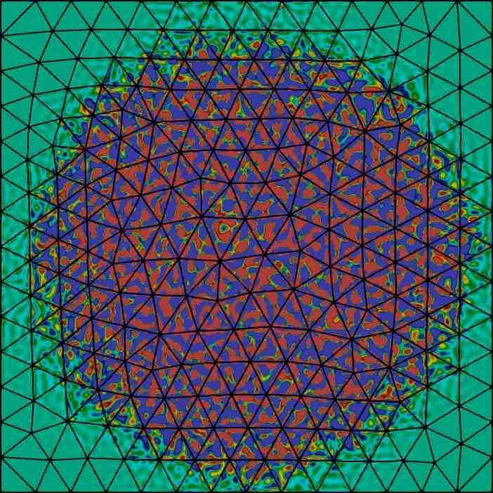
PRESSURE-ROBUSTNESS, HIGH REYNOLDS NUMBERS, BELTRAMI FLOWS

    (3) Finally, for generalised Beltrami flows the vorticity is neither zero, nor parallel to the flow field,
        but the Lamb vector is a gradient field
                                                 ω × u = ∇φ.                                               (2.5)

                                                                             1     2
        Here, the pressure gradient is different, namely ∇p = −∇             2 |u|     +φ .

It should be remarked that the vorticity equation of a generalised Beltrami flow (with f = 0) is linear
and given by
                                           ∂t ω − ν∆ω = 0.                                        (2.6)
Thus, a generalised Beltrami flow with f = 0 and time-independent boundary conditions presents a
nearly-steady behaviour over long time intervals, at least for small kinematic viscosities ν  1. As a
first connection to vortex-dominated flows, we remark that the slow decay of vortex structures like the
2D planar lattice flow problem is modelled by such flows [59]. For such a process, a steady Eulerian
description is sufficient.

2.3. Galilean invariance and the material derivative
In this short subsection, we briefly want to discuss the role of the divergence-free part of the nonlinear
convection term (u · ∇)u. It enters the game whenever a steady Eulerian description is not sufficient
anymore.

Recalling that the incompressible Navier–Stokes equations are Galilean-invariant, we start from a
generalised Beltrami flow (u0 , p0 ), fulfilling
                          ∂t u0 − ν∆u0 + (u0 · ∇)u0 + ∇p0 = 0,            ∇ · u0 = 0,
and add a constant velocity field w0 such that one obtains a new flow field
                                       u(t, x) = w0 + u0 (t, x − tw0 ).
Below, the corresponding pressure will be demonstrated to be
                                           p(t, x) = p0 (t, x − tw0 ).
Then, one computes
               ∂t u(t, x) = ∂t [u0 (t, x − tw0 )] = ∂t u0 (t, x − tw0 ) − (w0 · ∇)u0 (t, x − tw0 )
and
       (u(t, x) · ∇)u(t, x) = (w0 + u0 (t, x − tw0 ) · ∇)u0 (t, x − tw0 )                                (2.7a)
                             = (w0 · ∇)u0 (t, x − tw0 ) + (u0 (t, x − tw0 ) · ∇)u0 (t, x − tw0 ).        (2.7b)
Therefore, for the material derivative of u it holds
 Du(t, x)
           := ∂t u(t, x) + (u(t, x) · ∇)u(t, x) = ∂t u0 (t, x − tw0 ) + (u0 (t, x − tw0 ) · ∇)u0 (t, x − tw0 ),
    Dt
which is invariant under the Galilean transformation. Since it further holds
                                     −ν∆u(t, x) = −ν∆u0 (t, x − tw0 )
and ∇ · u(t, x) = 0, the pair (u(t, x), p(t, x)) does indeed fulfil the incompressible Navier–Stokes equa-
tions with f = 0.

                                                       5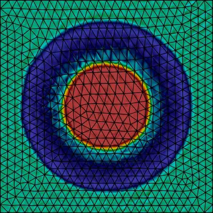
N.R. Gauger, A. Linke, & P.W. Schroeder

Besides the gradient part (u0 (t, x − tw0 ) · ∇)u0 (t, x − tw0 ) (due to the generalised Beltrami property
of u0 ), the transformed nonlinear convection term (2.7) does contain the new contribution (w0 · ∇)u =
∇u0 (t, x − tw0 )w0 . For this contribution, it holds
                   ∇ · (∇u0 (t, x − tw0 )w0 ) = ∇ · ((w0 · ∇)u) = (w0 · ∇)(∇ · u) = 0.
Thus, the nonlinear convection term of flows that are Galilean-invariant to a generalised Beltrami flow
contains both a divergence-free and a gradient-field part. The corresponding vorticity equation remains
linear, but contains an additional linear convection term
                                       ∂t ω − ν∆ω + (w0 · ∇)ω = 0.                                      (2.8)
By means of an example in the next subsection we will demonstrate that the divergence-free part of
the nonlinear convection term is responsible for the transport of geometric structures in the flow (like
vortices, vortex filaments, . . . ), while the gradient field part prevents the dispersion of geometric struc-
tures, thereby ensuring conservation of mass. Thus, the gradient field part of the nonlinear convection
term is of major importance for incompressible high Reynolds number flows, although it represents a
challenge for non-pressure-robust space discretisations.

2.4. Steady solutions of the incompressible Euler equations, Galilean invariance and the
     Euler material derivative
In this subsection we will slightly go beyond generalised Beltrami flows with f = 0 and discuss the
limit case Re → ∞, leading to the incompressible Euler equations with f = 0; that is,

                                        ∂t u + (u · ∇)u + ∇p = 0,
                                                          ∇ · u = 0.
First, we want to remind the reader that vortices, vortex lines and vortex filaments are the building
blocks of fluid dynamics [18]. Vortex-like solutions can be obtained as steady solutions of the incom-
pressible Euler equations (2.9), for which it holds
                                             (u · ∇)u = −∇p.
Thus, every steady solution u of the incompressible Euler equations has a nonlinear convection term
which is velocity-equivalent to a zero force,
                                               (u · ∇)u ' 0,
in the sense of corresponding equivalence classes of forces as introduced above. In the frictionless Euler
setting, there exist even steady solutions with a compact support like the famous Gresho vortex, see
Section 6. Indeed, for steady solutions of the incompressible Euler equations with a compact support
mainly the centrifugal force and the pressure gradient balance, similar to a tornado. Self-evidently,
the centrifugal force is modelled by the (quadratic) convection term of the incompressible Euler and
Navier–Stokes equations. We remark that steady solutions of the incompressible Euler equations can
contain an immense amount of kinetic energy, which is contained in rotational degrees of freedom,
though. This rotational kinetic energy can be unleashed, whenever vortices or vortex filaments interact
with each other or interact with the boundary of the domain.

Since all considerations from Subsection 2.3 about the Galilean invariance of the incompressible Navier–
Stokes equations are valid for the Euler equations as well, the divergence-free part of the nonlinear
convection term leads to a transport of structures; cf. the example of the Gresho vortex in Section 6
in the case w0 6= 0.

                                                      6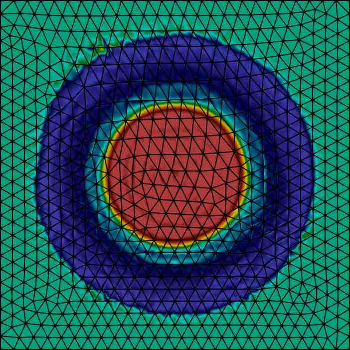
PRESSURE-ROBUSTNESS, HIGH REYNOLDS NUMBERS, BELTRAMI FLOWS
Moreover, looking at (2.9), we recognise that for the material derivative of incompressible Euler flows
with f = 0 it holds
Du
= ∂t u + (u · ∇)u = −∇p, (2.10)
Dt
i.e., for the Euler material derivative one obtains
Du
' 0. (2.11)
Dt
Thus, strong forces of gradient field type are typical for incompressible Euler and Navier–Stokes flows
at high Reynolds numbers, e.g., due to a force balance of the nonlinear centrifugal force and a strong,
nontrivial pressure gradient.
The next subsection serves to illustrate that strong and ‘complicated’ gradient fields in the Navier–
Stokes momentum balance lead to numerical errors for non-pressure-robust space discretisations, while
pressure-robust discretisations behave well.
2.5. Hydrostatics: Complicated pressure
Let us explain in more detail, what we usually mean by ‘complicated pressures’. The most important
point is that ‘complicated’ is always meant compared to the velocity. In this sense, a complicated pres-
sure in a particular flow is always a relative concept.
In hydrostatics (flow at rest, no-flow), the pressure usually balances an external (gradient) force field,
which makes it a perfect example for presenting ‘complicated pressures’. For ease of presentation, sup-
pose we want
R to solve the incompressible Stokes problem (ν = 1), with a right-hand side forcing term
f = ∇φ/ Ω φ. Here, the normalisation is made to ensure comparable situations for different potentials
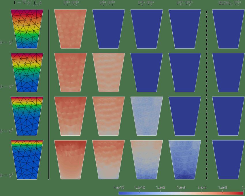
φ. The left-hand side column in Figure 1 shows different potentials φ = y γ for γ = 1, 2, 4, 9 in a domain
Ω which resembles a glass geometry. Note that the pressure behaves analogously as these potentials
and thus, they can be considered ‘complicated’ compared to the exact velocity solution u = 0 in hy-
drostatics problems.
Now, all other plots in Figure 1 show the velocity solution of different numerical methods for the par-
ticular problem. The chosen methods are L2 - (PP dc dc BDM 1 /Pdc
k /Pk−1 ) and H(div)-based (BDM 0 ) DG methods
on triangular meshes of different order k (polynomial order of the discrete velocity approximations),
In the present context, it suffices to know that the former are non-pressure-robust whereas the latter
are pressure-robust and divergence-free; cf. Section 7 for more details.
One can see that the low-order (k = 1) pressure-robust method computes the correct velocity solution
uh = 0 independent of the pressure/potential, even though the discrete pressure space only consists
of piecewise constants. The non-pressure-robust method, on the other hand, only leads to uh = 0 if
k − 1 > γ, as in this situation the pair (u, p) is contained in the discrete FE spaces. Moreover, one can
see that whenever the non-pressure-robust method gives uh 6= 0, the quality of the solution decreases
as γ increases, i.e. as the pressure becomes more and more complicated. On the other hand, increasing
the order k of the discretisation improves the solution; this is simply k-convergence.
3. Time-dependent Navier–Stokes problem and H1 discretisation
After a very brief introduction to the governing equations on the continuous level, we introduce the
spatial H 1 -conforming discretisation schemes which will be used for the error analysis in the first
7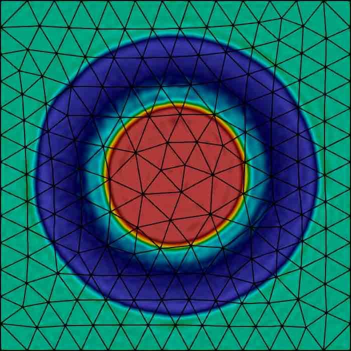
N.R. Gauger, A. Linke, & P.W. Schroeder
Figure 1. Stokes no-flow problem in a glass, demonstrating the concept of complex
pressures and the advantages of using pressure-robust methods. The left-hand side
column shows the potential φ = y γ for γ = 1, 2, 4, 9 and the underlying triangu-
lar mesh for all computations. The other columns show velocity magnitude |uh | for
the non-pressure-robust P dc dc
k /Pk−1 method and the pressure-robust and divergence-free
BDM 1 /Pdc
0 method.
part of this work. They consist of an exactly divergence-free, pressure-robust method and a classical
non-pressure-robust FEM.
3.1. Infinite-dimensional Navier–Stokes equations
We consider the time-dependent incompressible Navier–Stokes problem, which reads
∂t u − ν∆u + (u · ∇)u + ∇p = f
in (0, T ] × Ω,
∇·u = 0 in (0, T ] × Ω,
u(0, x) = u0 (x) for x ∈ Ω.
For the space dimension d ∈ {2, 3}, Ω ⊂ Rd denotes a connected bounded Lipschitz domain and T is
the end of time considered in the particular problem. Since in the numerical analysis below we want
to compare the best possible convergence rates for pressure-robust and classical space discretisations
8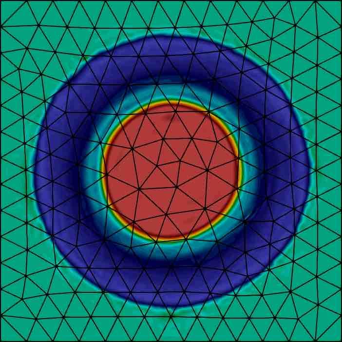
PRESSURE-ROBUSTNESS, HIGH REYNOLDS NUMBERS, BELTRAMI FLOWS

in the L2 -norm, we will assume for technical reasons that Ω is convex, leading to elliptic regularity.
Moreover, u : [0, T ]×Ω → Rd indicates the velocity field, p : [0, T ]×Ω → R is the (zero-mean) kinematic
pressure, f : [0, T ] × Ω → Rd represents external body forces and u0 : Ω → Rd stands for a suitable
initial condition for the velocity. The underlying fluid is assumed to be Newtonian with constant
(dimensionless) kinematic viscosity 0 < ν  1. We impose either the general Dirichlet boundary
condition u = gD on (0, T ] × ∂Ω, or periodic boundary conditions (or a mixture of them).

Notation. In what follows, for K ⊆ Ω we use the standard Sobolev spaces W m,p (K) for scalar-valued
functions with associated norms k·kW m,p (K) and seminorms |·|W m,p (K) for m > 0 and p > 1. We obtain
the Lebesgue space W 0,p (K) = Lp (K) and the Hilbert space W m,2 (K) = H m (K). Additionally, the
closed subspaces H01 (K) consisting of H 1 (K)-functions with vanishing trace on ∂K and the set L20 (K)
of L2 (K)-functions with zero mean in K play an important role. The L2 (K)-inner product is denoted
by (·, ·)K and, if K = Ω, we sometimes omit the domain completely when no confusion can arise. Fur-
thermore, with regard to time-dependent problems, given a Banach space X and a time instance t, the
Bochner space Lp (0, t; X) for p ∈ [1, ∞] is used. In the case t = T , we frequently use the abbreviation
Lp (X) = Lp (0, T ; X). Further, C 1 (0, t; X) denotes the function space mapping [0, t] into X, which
is continuously differentiable in time w.r.t. the norm kukC 1 (0,t;X) maxs∈[0,T ] (kukX + kut kX ). Spaces
and norms for vector- and tensor-valued functions are indicated with bold letters. For       R example, for a
                                                                          P
vector-valued function v = (v1 , . . . , vn )† , we consider kvkpLp (Ω) = ni=1 kvi kpLp (Ω) = Ω |v|pp dx, where
        P
|v|pp = ni=1 |vi |p . The vorticity of a 2D velocity field u = (u1 , u2 )† is defined as ω = ∂x1 u2 − ∂x2 u1 .

Depending on the particular boundary conditions, let V /Q be the continuous solution spaces for
velocity and pressure, respectively. Note that it holds V ⊂ H 1 (Ω) and Q ⊂ L2 (Ω). For the numerical
analysis in this and the next section, we will always choose V = H01 (Ω) and Qh = L20 (Ω). The subspace
of weakly divergence-free functions is defined as
                             V div = {v ∈ V : (q, ∇ · v) = 0, ∀ q ∈ Q}.

A weak velocity solution u ∈ L2 0, T ; V div of (3.1) fulfils that for all test functions v ∈ V div holds
                    d
                      (u(t), v) + ν(∇u(t), ∇v) + ((u(t) · ∇)u(t), v) = hf (t), viH −1 ,H 1            (3.2)
                   dt                                                                   0

in the sense of distributions in D0 (]0, T [) and such that u(0) = u0 [13]. Note that the pressure p is not
part of the weak formulation of the incompressible Navier–Stokes problem,        see Remark 3.6. For the
numerical analysis, we will further assume the regularity u ∈ L1 W 1,∞ , ensuring, e.g., uniqueness of
the weak solution in time [8, 61]. Further (technical) regularity assumptions will be made at appropriate
places in the contribution. Then, (u, p) fulfils
              (
                Find (u, p) : (0, T ] → V × Q with u(0) = u0 s.t., ∀ (v, q) ∈ V × Q,
                    (∂t u, v) + ν(∇u, ∇v) + ((u · ∇)u, v) − (p, ∇ · v) + (q, ∇ · u) = (f , v).

3.2. Helmholtz–Hodge decomposition in L2
In order to understand the significance of pressure-robustness for the discretisation theory of the
incompressible Navier–Stokes equations (3.1), the concept of the Helmholtz–Hodge projector is intro-
duced. Since the numerical analysis below is essentially an L2 analysis (assuming all forces ∂t u(t),
(u(t) · ∇)u(t), . . . to be in L2 ), we will restrict our considerations to the Helmholtz–Hodge decomposi-
tion in L2 . Below in this section, some functional analytic prerequisites are summarised that show that
only the divergence-free parts, i.e., the Helmholtz–Hodge projectors of the forces in the Navier–Stokes
momentum balance influence the velocity solution of the incompressible Navier–Stokes equations, see

                                                      9
N.R. Gauger, A. Linke, & P.W. Schroeder
also [42].
The space of square-integrable divergence-free (solenoidal) vector fields is defined by
L2σ (Ω) := w ∈ L2 (Ω) : − (w, ∇φ) = 0, ∀ φ ∈ H 1 (Ω) . (3.4)
Remark 3.1. First note that for φ ∈ C0∞ (Ω) the mapping φ 7→ −(w, ∇φ) denotes the distributional
divergence of w. Thus, vector fields in L2σ (Ω) are divergence-free [42]. Further note that definition (3.4)
implies that w · n ∂Ω = 0, where n denotes the outer unit normal vector on ∂Ω, since test functions
φ ∈ H 1 do not vanish on the boundary of Ω. In this context, please also note that a Helmholtz–Hodge
decomposition is made unique only by prescribing certain boundary conditions. The reason is that any
gradient of a harmonic function with −∆h = 0 is irrotational and divergence-free at the same time.
Thus, the boundary conditions determine whether ∇h is called ’divergence-free’ or ’gradient field’. In
our setting, all gradients of harmonic functions are called ’gradient fields’, and vector fields in L2σ (Ω)
are orthogonal to all gradient fields in L2 .
Remark 3.2. Our considerations regard the Helmholtz–Hodge decomposition in L2 of (u · ∇)u. Since
we assume that u ∈ W 1,∞ , it holds (u · ∇)u ∈ L2 .
Due to the special choice of the boundary conditions and Remark 3.1 one obtains the following theorem,
for which the proof will be repeated for completeness and readability of the manuscript from [42]:
Theorem 3.3 (Helmholtz–Hodge decomposition in L2 ). For every vector field v ∈ L2 (Ω), there exists
a unique Helmholtz–Hodge decomposition
v = w + ∇ψ, (3.5)
where it holds w ∈ L2σ (Ω),
and ψ ∈ H 1 (Ω) and w and ∇ψ are L2 -orthogonal. Then, w =: P(v) is
called the Helmholtz–Hodge projector of v.
Proof. A potential ψ ∈ H 1 (Ω)/R in the Helmholtz–Hodge decomposition is obtained by: for all
χ ∈ H 1 (Ω)/R holds
(∇ψ, ∇χ) = (v, ∇χ). (3.6)
This Neumann problem for ψ is uniquely solvable [42]. Then, define w := v − ∇ψ. One can test w
with arbitrary gradient fields ∇(φ + C), where C denotes an arbitrary real number and where it holds
φ ∈ H 1 (Ω)/R. Then, one obtains (w, ∇(φ + C)) = (w, ∇φ) = (v − ∇ψ, ∇φ) = 0, due to (3.6). Thus,
it holds w ∈ L2σ (Ω). Due to the definition of L2σ (Ω), w and ∇ψ are orthogonal in L2 . Assuming that
v = w1 + ∇ψ1 = w2 + ∇ψ2 are two Helmholtz–Hodge decompositions of v, then it holds
w1 − w2 = ∇(ψ2 − ψ1 )
with w1 − w2 ∈ Lσ (Ω). Testing this equality by ∇(ψ1 − ψ2 ) yields by the L2 -orthogonality of (3.6)
2
k∇(ψ2 − ψ1 )k2L2 (Ω) = 0,
and one concludes w1 = w2 and ψ1 = ψ2 using ψ1 , ψ2 ∈ H 1 (Ω)/R. Thus, the Helmholtz–Hodge
decomposition is unique.
Remark 3.4. Formally, the Helmholtz–Hodge decomposition of v ∈ L2 (Ω) can be written as the
solution of the PDE problem
P(v) + ∇ψ = v
in Ω,
∇ · P(v) = 0 in Ω,
P(v) · n = 0 on ∂Ω.
The most important property of the Helmholtz–Hodge projector for our contribution is given as follows:
10PRESSURE-ROBUSTNESS, HIGH REYNOLDS NUMBERS, BELTRAMI FLOWS
Lemma 3.5. For all ψ ∈ H 1 (Ω), it holds
P(∇ψ) = 0.
Proof. Note that ∇ψ = 0+∇ψ is the unique Helmholtz–Hodge decomposition of ∇ψ. Thus, it follows
P(∇ψ) = 0.
Finally, it is emphasised that the velocity solution u of (3.2) is completely determined by testing the
momentum equation with divergence-free velocity test functions v ∈ V div and by its initial value u0 .
Assuming smoothness of u in space and time, u fulfils for all v ∈ V div
(∂t u, v) + ν(∇u, ∇v) + ((u · ∇)u, v) = (f , v) ⇔ (3.8a)
(P(∂t u), v) − ν(P(∆u), v) + (P((u · ∇)u), v) = (P(f ), v). (3.8b)
Remark 3.6. Equation (3.8a) shows that the velocity solution u of the incompressible Navier–Stokes
equations is not determined by the forces f in the momentum equation themselves, but by their
Helmholtz–Hodge projectors P(f ). Therefore, two forces f and g that differ by a gradient field f =
g + ∇φ, lead to the same velocity solution. Thus, the velocity solution of the incompressible Navier–
Stokes equations is naturally determined by equivalence classes of forces, where it holds
f 'g ⇔ P(f ) = P(g).
3.3. H1 finite element methods
Let Vh /Qh be the considered discretely inf-sup stable velocity/pressure FE pair, where Vh ⊂ V and
Qh ⊂ Q. We assume that the discrete velocity space contains polynomials up to degree ku and the
discrete pressure space contains polynomials up to degree kp . Note that for most discretely inf-sup
stable schemes it holds kp = ku − 1. An example is the Taylor–Hood finite element family P k /Pk−1
with k > 2 [41]. However, for the famous mini element it holds kp = ku (= 1) [5]. In the following
numerical analysis, C > 0 always denotes a generic constant, whose value is independent of the mesh
size but possibly dependent on the mesh-regularity.
In order to approximate (3.1), or equivalently (3.3), the following generic semi-discrete FEM is consid-
ered:
Find (uh , ph ) : (0, T ] → Vh × Q
h with uh (0) = u0h s.t., ∀ (vh , qh ) ∈ Vh × Qh ,
1
(∂t uh , vh ) + ν(∇uh , ∇vh ) + (uh · ∇)uh + (∇ · uh )uh , vh − (ph , ∇ · vh ) = (f , vh )
2
(qh , ∇ · uh ) = 0.
Now, the choice of the FE spaces decides whether an exactly divergence-free, pressure-robust method
is applied or not. For example, the Scott–Vogelius element P k /Pdc k−1 is discretely inf-sup stable on
shape-regular, barycentrically refined meshes for k > d [65], or on meshes without singular vertices for
k > 2d; then it yields an exactly divergence-free and thus pressure-robust method. On the other hand,
for example, a classical P k /Pk−1 Taylor–Hood element is a non-pressure-robust method. Note that the
explicit skew-symmetrisation of the convective term is only necessary for a non-divergence-free FEM.
The subspace of discretely divergence-free functions is given by
Vhdiv = {vh ∈ Vh : (qh , ∇ · vh ) = 0, ∀ qh ∈ Qh },
11N.R. Gauger, A. Linke, & P.W. Schroeder
where we note that for exactly divergence-free (and thus pressure-robust) FEM, vh ∈ Vhdiv follows
∇ · vh = 0, i.e., Vhdiv ⊂ L2σ (Ω). In this context, a frequently used tool in finite element error analysis
is the discrete Stokes projector, defined by
Z
div div
Sh : V → Vh , Sh (v) = arg min k∇(v − vh )kL2 (Ω) , ∇[S(v) − v] : ∇vh dx = 0, ∀ vh ∈ Vhdiv .
vh ∈Vhdiv Ω
The Stokes projector possesses optimal approximation properties due to discrete inf-sup stability [1].
Last but not least, the Lagrange interpolation into the H 1 -conforming subspace of the discrete pressure-
space Qh is denoted by
Lh : C(Ω̄) → Qh ∩ H 1 (Ω). (3.10)
Remark 3.7. For discrete discontinuous pressure spaces with kp > 1 it holds for all q ∈ H kp +1
k∇(q − Lh q)kL2 6 Chkp |q|H kp +1 (Ω) ,
where C does only depend on the shape-regularity of the triangulation.
Lemma 3.8 (Convergence of the nonlinear convection term as h → 0). Assume that uh → u ∈
W 1,∞ (Ω) converges strongly in H 1 (Ω) and that kuh kW 1,∞ (Ω) 6 C is uniformly bounded. Then,
(uh · ∇)uh → (u · ∇)u converges strongly in L2 (Ω). Further, it holds that P((uh · ∇)uh ) → P((u · ∇)u)
converges strongly for the Helmholtz–Hodge projector in L2 (Ω).
Proof. One can derive
k(uh · ∇)uh − (u · ∇)ukL2 (Ω) 6 k((uh − u) · ∇)uh kL2 (Ω) + k(u · ∇)(uh − u)kL2 (Ω)
6 kuh − ukL2 (Ω) k∇uh kL∞ (Ω) + kukL∞ (Ω) k∇(uh − u)kL2 (Ω) .
Due to uh → u strongly in H 1 (Ω),
kuh − ukL2 (Ω) and k∇(uh − u)kL2 (Ω) converge to zero. Further,
k∇uh kL∞ (Ω) and kukL∞ (Ω) are assumed to be bounded. The convergence of the Helmholtz–Hodge
projectors P((uh · ∇)uh ) → P((u · ∇)u) in L2 (Ω) is an immediate consequence of the well-posedness
of the Neumann problem (3.6) in H 1 (Ω)/R.
Remark 3.9 (Pseudo-dominant convection). When confronted with generalised Beltrami flows at high
Reynolds numbers, Lemma 3.8 is decisive in order to understand the behaviour of space discretisations
of the incompressible Navier–Stokes equations. While P((u · ∇)u)) vanishes for generalised Beltrami
flows since (u · ∇)u is a gradient field, on the discrete level P((uh · ∇)uh )) → 0 holds since (uh · ∇)uh
only converges to a gradient field as h → 0. Thus, one can observe some kind of pseudo-dominant
convection at high Reynolds numbers [48], i.e., the infinite-dimensional generalised Beltrami problem
is not convection-dominated due to P((u · ∇)u)) = 0, but the discretised problem experiences some
non-negligible, artificial convective force. A similar effect can be observed also for the linear Stokes
problem when one uses numerical quadratures in the discretisation of forces of gradient fields, see [50,
Subsection 6.2].
3.4. Discrete H1 -conforming Helmholtz–Hodge projector
A discrete Helmholtz–Hodge projector in L2 is defined straightforward as the L2 projector onto Vhdiv :
Z
2 div
Ph : L (Ω) → Vh , Ph (v) = arg min kv − vh kL2 (Ω) , [Ph (v) − v] · vh dx = 0, ∀ vh ∈ Vhdiv .
vh ∈Vhdiv Ω
(3.11)
12PRESSURE-ROBUSTNESS, HIGH REYNOLDS NUMBERS, BELTRAMI FLOWS
Remark 3.10. Under the assumptions of elliptic regularity of Ω, shape-regular meshes and discrete inf-
sup stability of the method, the corresponding discrete Helmholtz projector has optimal approximation
properties
ku − Ph (u)kL2 (Ω) + h k∇[u − Ph (u)]kL2 (Ω) 6 Chk+1 kukH k+1 (Ω) . (3.12)
The proof follows directly from [1, Lemma 11].
Lemma 3.11 (W 1,∞ stability of discrete Helmholtz–Hodge projector). Assume elliptic regularity of Ω,
shape-regular meshes, discrete inf-sup stability of the method and that the exact solution u is sufficiently
smooth. Then, the corresponding discrete Helmholtz–Hodge projector fulfils
k∇Ph (u)kL∞ (Ω) 6 C k∇ukL∞ (Ω) + hku − /2 kukH ku +1 (Ω) ,
d
(3.13)
where C > 0 is independent of h and ku denotes the polynomial order of discrete velocities in Vh .
Proof. The first step is to use the Stokes projector and the triangle inequality to obtain
k∇Ph (u)kL∞ (Ω) 6 k∇Sh (u)kL∞ (Ω) + k∇Ph (u) − ∇Sh (u)kL∞ (Ω) .
Note that the W 1,∞ stability of the Stokes projector has been shown in [36]. For shape-regular de-
compositions Th , the discrete space Vh (and thus also Vhdiv ) satisfies the local inverse inequality [27,
Lemma 1.138]
m−`+d p1 − 1q
∀vh ∈ Vh : kvh kW `,p (K) 6 Cinv hK kvh kW m,q (K) , ∀K ∈ Th , (3.14)
where 0 6 m 6 ` and 1 6 p, q 6 ∞. Choosing ` = m = 1, p = ∞ and q = 2, the inverse estimate can
be applied to further estimate the right-hand side as
k∇Ph (u) − ∇Sh (u)kL∞ (Ω) 6 Cinv h− /2 k∇[Ph (u) − Sh (u)]kL2 (Ω)
d
h i
6 Cinv h− /2 k∇[u − Ph (u)]kL2 (Ω) + k∇[u − Sh (u)]kL2 (Ω)
d
6 Chku − /2 kukH ku +1 (Ω) ,
d
where the optimal approximation properties of both Ph and Sh are essential.
Combining Lemmas 3.11 and 3.8 yields a result which is essential for good convergence properties of
the Galerkin method on pre-asymptotic meshes, see also Theorems 4.1 and 4.6:
Remark 3.12. Assuming ku > d/2, it holds for h → 0 that
L2
P((Ph (u) · ∇)Ph (u)) → P((u · ∇)u).
Now, let us first consider the situation where Ph belongs to a pressure-robust (divergence-free) method.
Lemma 3.13. For pressure-robust (divergence-free) H 1 methods, for all ψ ∈ H 1 (Ω) it holds
Ph (∇ψ) = 0.
Proof. Since for divergence-free methods ∇ · vh = 0 holds for all vh ∈ Vhdiv , one obtains
(∇ψ, vh ) = −(ψ, ∇ · vh ) = 0,
div
for all vh ∈ Vh .
Finally, for non-pressure-robust methods, the situation is not exactly the same as in the infinite-
dimensional case. In fact, for the steady Navier–Stokes problem, i.e., for the elliptic problem, one
has to estimate the consistency error of Ph (∇φ) in a discrete Hh−1 norm, which yields an O(hkp +1 )
consistency error [49], where kp denotes the formal approximation order of the discrete pressure space
in the L2 norm. However, for the fully time-dependent a priori error analysis below we will have to
13N.R. Gauger, A. Linke, & P.W. Schroeder
estimate this consistency error in the stronger L2 (Ω) norm, which was seemingly done for the first
time in [51].
Lemma 3.14. For non-pressure-robust H 1 methods with kp > 1, it holds for all gradient fields ∇ψ
with ψ ∈ H kp +1 (Ω)
kPh (∇ψ)kL2 (Ω) 6 Chkp |ψ|H kp +1 (Ω) . (3.15)
Proof. Given ψ ∈ H kp +1 (Ω), it holds for all discretely divergence-free vh ∈ Vhdiv
0 = −(Lh ψ, ∇ · vh ) = (∇(Lh ψ), vh ),
1
due to Lh ψ ∈ Qh ∩ H (Ω). Thus, one obtains
(∇ψ, vh ) = (∇(ψ − Lh ψ), vh ) 6 k∇(ψ − Lh ψ)kL2 (Ω) kvh kL2 (Ω) .
The result is proven using Remark 3.7.
Remark 3.15. The numerical experiments in [51] indicate that Lemma 3.14 is sharp. Indeed, for
non-pressure-robust, inf-sup stable mixed methods with discontinuous P0 pressures, i.e., kp = 0, like
the nonconforming Crouzeix–Raviart and the conforming Bernardi–Raugel element, it is demonstrated
that it holds
kPh (∇q)kL2 (Ω) = O(1),
leading to a pressure-induced locking phenomenon for the time-dependent Stokes equations in the
presence of large pressure gradients.
Remark 3.16. Remark 3.12 assures that at least for ku > d/2 one obtains for h → 0 the convergence
result
L2
P((Ph (u) · ∇)Ph (u)) → P((u · ∇)u).
However, the quality of the space discretisation (3.9) is determined by whether and how
L2
Ph ((Ph (u) · ∇)Ph (u)) → P((u · ∇)u)
converges for h → 0. For kp > 2, convergence in L2 is assured. But the convergence speed of pressure-
robust methods can be much faster than in classical, non-pressure-robust space discretisations due to
Lemma 3.14, when (u · ∇)u contains a large gradient part in the sense of the Helmholtz–Hodge decom-
position (3.5). This is the main reason for the superiority of pressure-robust methods for Beltrami flows,
where space discretisations suffer from an artificial, pseudo-dominant convection on coarse meshes, see
Remark 3.9. Exactly this artificial pseudo-dominant convection is reduced by pressure-robust methods.
4. A special H1 finite element error analysis
In the following, we present a numerical error analysis for the time-dependent Navier–Stokes problem
which is based on a new understanding of the velocity error in the time-dependent Stokes problem, see
[51] and [1, Section 4]. The key point is that in the case of low viscosities, pressure-robust space dis-
cretisations do not show an increase in the velocity error as long as the time interval is small compared
with ν −1 . On the other hand, in non-pressure-robust methods the only source of error is a dominating
pressure gradient in the momentum balance [2, Theorem 5.2]; namely in the special case f = const
one gets (for ν
1) uh ≈ Ph (u) + tPh (∇p) for t ∈ [0, T ].
In the following, we will give two different error estimates for the Navier–Stokes equations in the
pressure-robust and the non-pressure-robust case. The convergence analysis is inspired by novel discrete
velocity error estimates for the transient Stokes equations [51, 49, 1], which estimate the difference
between the discrete velocity uh (t) and the (discretely divergence-free) L2 best approximation Ph (u(t)).
14PRESSURE-ROBUSTNESS, HIGH REYNOLDS NUMBERS, BELTRAMI FLOWS
4.1. Pressure-robust space discretisation
Theorem 4.1 (Pressure-robust estimate). For the discrete velocity for all t ∈ [0, T ] the following
representation is chosen
uh (t) = Ph (u(t)) + eh (t),
and the time-dependent evolution of eh (t) is considered. Then, assuming u ∈ L2 W 1,∞ ∩ H 3 , ∂t u ∈
L1 L2 , on the time interval [0, T ], eh can be estimated by
1+2k∇Ph (u)kL1 (L∞ )
keh (T )k2L2 + ν k∇eh k2L2 (L2 ) 6 e × ν k∇[Sh (u) − Ph (u)]k2L2 (L2 )
Z T
+2T k∇Ph (u)k2L∞ ku − Ph (u)k2L2 + kuk2L∞ k∇[u − Ph (u)]k2L2 dτ .
0
Remark 4.2. Due to the explicit 2T dependence of the error in Theorem 4.1, in the case T
ν −1
this estimate can become pessimistic. Note that for our numerical examples in Section 8, we indeed
consider short time intervals for which Theorem 4.1 is meaningful. In the literature, usually one can find
’long-term’ estimates, e.g., [9, 16, 4, 61, 60], which are sharper for T
ν −1 , but which are pessimistic
for short time intervals.
Remark 4.3. Concerning the regularity assumption u ∈ L2 H 3 in Theorem 4.1, let us remark that
we have chosen it in such a way that the stability of the discrete Helmholtz projector in Lemma 3.11 is
ensured. This is basically a technical detail and with additional effort, one can presumably reduce the
necessary regularity at this point. However, in the error analysis of this work, we are only interested
in relatively smooth flows anyway.
Proof of Theorem 4.1. Note that ∇ · zh = 0 for all zh ∈ Vhdiv due to Vhdiv ⊂ L2σ (Ω) assuming
pressure-robustness. Due to Galerkin orthogonality, for all zh ∈ Vhdiv it holds
(∂t uh , zh ) + ν(∇uh , ∇zh ) + ((uh · ∇)uh , zh ) = (∂t u, zh ) + ν(∇u, ∇zh ) + ((u · ∇)u, zh )
= (∂t Ph (u), zh ) + ν(∇Sh (u), ∇zh ) + ((u · ∇)u, zh ).
Here, it was used (∇p, zh ) = 0, which is equivalent to Ph (∇p) = 0, proved in Lemma 3.13 for pressure-
robust space discretisations. Using the representation uh (t) = Ph (u(t)) + eh (t) leads to
(∂t eh , zh ) + ν(∇eh , ∇zh ) + (([Ph (u) + eh ] · ∇)[Ph (u) + eh ], zh )
= ν(∇(Sh (u) − Ph (u)), ∇zh ) + ((u · ∇)u, zh ),
for all zh ∈Vhdiv , where the initial value for the ODE system is chosen as eh (0) = 0. For the discrete
nonlinear term, we obtain
(([Ph (u) + eh ] · ∇)[Ph (u) + eh ], zh ) =((eh · ∇)eh , zh ) + ((Ph (u) · ∇)eh , zh )
+ ((eh · ∇)Ph (u), zh ) + ((Ph (u) · ∇)Ph (u), zh ).
Further, due to the skew-symmetry of the first two terms plus ∇ · eh = ∇ · Ph (u) = 0, testing with
zh = eh leads to
1d
keh k2L2 + ν k∇eh k2L2
2 dt
= ν(∇[Sh (u) − Ph (u)], ∇eh ) − ((eh · ∇)Ph (u), eh ) − ((Ph (u) · ∇)Ph (u), eh ) + ((u · ∇)u, eh ).
Due to Lemmas 3.8 and 3.11, the last two terms on the right-hand side can be combined and estimated
by
(Ph (u) · ∇)Ph (u) − (u · ∇)u, eh = (([Ph (u) − u] · ∇)Ph (u) + (u · ∇)[Ph (u) − u], eh )
6 k∇Ph (u)kL∞ ku − Ph (u)kL2 keh kL2 + kukL∞ k∇[u − Ph (u)]kL2 keh kL2
1
6 T k∇Ph (u)k2L∞ ku − Ph (u)k2L2 + kuk2L∞ k∇[u − Ph (u)]k2L2 + keh k2L2 .
2T
15N.R. Gauger, A. Linke, & P.W. Schroeder
Here, the weight (2T )−1 in front of keh k2L2 ensures that later on, the argument of the exponential
Gronwall term does not catch any explicit T dependence. The other convection term can be treated
simply by the generalised Hölder inequality; that is,
((eh · ∇)Ph (u), eh ) 6 k∇Ph (u)kL∞ keh k2L2 .
Using Young’s inequality for the remaining term involving Stokes and Helmholtz–Hodge projectors,
after rearranging, one obtains the overall estimate
d 2 2 2 1
keh kL2 + ν k∇eh kL2 6ν k∇[Sh (u) − Ph (u)]kL2 + + 2 k∇Ph (u)kL∞ keh k2L2
dt T
+ 2T k∇Ph (u)k2L∞ ku − Ph (u)k2L2 + kuk2L∞ k∇[u − Ph (u)]k2L2 .
In such a situation, Gronwall’s lemma [41, Lemma A.54] in differential form states that for t ∈ [0, T ],
Z t Z t
d 2 2 2
keh (t)kL2 6 α(t) + β(t) keh (t)kL2 ⇒ keh (t)kL2 6 α(s) exp β(τ ) dτ ds. (4.1)
dt 0 s
In order to apply this estimate, one sets
1
β(t) = + 2 k∇Ph (u)kL∞
T
and
α(t) = − ν k∇eh k2L2 + ν k∇[Sh (u) − Ph (u)]k2L2
+ 2T k∇Ph (u)k2L∞ ku − Ph (u)k2L2 + kuk2L∞ k∇[u − Ph (u)]k2L2 ,
and computes for t > s
Z t
t−s
exp β(τ ) dτ = exp + 2 k∇Ph (u)kL1 (s,t;L∞ ) .
s T
Using 0 6 s 6 t 6 T and 0 6 t−s T 6 1, one obtains
(
t−s c exp 1 + 2 k∇Ph (u)kL1 (L∞ ) for c > 0,
c exp + 2 k∇Ph (u)kL1 (s,t;L∞ ) 6
T c for c < 0.
Now, actually applying Gronwall’s lemma yields the estimate
Z T Z T
2 1+2k∇Ph (u)kL1 (L∞ )
keh (T )kL2 6 α(s) exp β(τ ) dτ ds 6 −ν k∇eh k2L2 (L2 ) + e ×
0 s
Z T
2 2 2 2 2
ν k∇[Sh (u) − Ph (u)]kL2 (L2 ) + 2T k∇Ph (u)kL∞ ku − Ph (u)kL2 + kukL∞ k∇[u − Ph (u)]kL2 dτ .
0
Rearranging concludes the proof.
Remark 4.4. The estimate in Theorem 4.1 is pressure-robust, since if u(t) ∈ Vhdiv holds for all
t ∈ [0, T ], then it also holds uh (t) = u(t) due to u = Sh (u) = Ph (u), i.e., the pressure p does not spoil
the discrete velocity solution uh .
Remark 4.5. Note that under the assumption that ku is large enough and h is small enough, one can
apply Lemma 3.11 to obtain k∇Ph (u)kL∞ 6 C k∇ukL∞ .
4.2. Classical space discretisation
Theorem 4.6 (Non-pressure-robust estimate). For the discrete velocity for all t ∈ [0, T ] the following
representation is chosen
uh (t) = Ph (u(t)) + eh (t),
16PRESSURE-ROBUSTNESS, HIGH REYNOLDS NUMBERS, BELTRAMI FLOWS
and the time-dependent evolution of eh (t) is considered. Then, assuming u ∈ L2 W 1,∞ ∩ H 3 , ∂t u ∈
L1 L2 , p ∈ L2 H 1 , on the time interval [0, T ], eh can be estimated by
1+4k∇Ph (u)kL1 (L∞ )
keh (T )k2L2 + ν k∇eh k2L2 (L2 ) 6 e × ν k∇[Sh (u) − Ph (u)]k2L2 (L2 )
Z T
2
+ 3T k∇[p − Lh (p)]kL2 (L2 ) + 3T kPh (u)k2L∞ k∇ · Ph (u)k2L2
0
+ 2 k∇Ph (u)kL∞ ku − Ph (u)k2L2 + 2 kuk2L∞ k∇[u − Ph (u)]k2L2 dτ .
2
Proof of Theorem 4.6. Following the same procedure as for the pressure-robust case, one obtains
1d
keh k2L2 + ν k∇eh k2L2 = ν(∇[Sh (u) − Ph (u)], ∇eh ) + (∇[p − Lh (p)], eh ) + ((u · ∇)u, eh )
2 dt
1 1
− (eh · ∇)Ph (u) + (∇ · eh )Ph (u), eh − (Ph (u) · ∇)Ph (u) + (∇ · Ph (u))Ph (u), eh .
2 2
Note that in the non-pressure-robust case the pressure contribution does not vanish, since it holds
Vhdiv 6⊂ L2σ (Ω) and the consistency error kPh (∇p)kL2 (Ω) estimated in Lemma 3.14 unavoidably appears
in the estimate. Further, the full skew-symmetric convective term has to be taken into account. In com-
parison to the pressure-robust case, there are only two new contributions from the skew-symmetrisation
of the convective term which have to be estimated. For the first one,
1 1
(∇ · Ph (u))Ph (u), eh = (∇ · [u − Ph (u)])Ph (u), eh 6 kPh (u)kL∞ k∇ · [u − Ph (u)]kL2 keh kL2
2 2
3T 1
6 kPh (u)k2L∞ k∇ · [u − Ph (u)]k2L2 + keh k2L2
2 6T
can be obtained. Applying Young’s inequality slightly differently than in the pressure-robust case leads
to
(Ph (u) · ∇)Ph (u) − (u · ∇)u, eh
6T 1
6 k∇Ph (u)k2L∞ ku − Ph (u)k2L2 + kuk2L∞ k∇[u − Ph (u)]k2L2 + keh k2L2 .
2 6T
With the help of integration by parts, the additional contribution in the remaining additional convective
term can be estimated
as
1 1
(∇ · eh )Ph (u), eh = − ((∇Ph (u))eh , eh ) 6 k∇Ph (u)kL∞ keh k2L2 .
2 2
For completeness, from the pressure-robust case, we repeat
((eh · ∇)Ph (u), eh ) 6 k∇Ph (u)kL∞ keh k2L2 .
Finally, the additional pressure term can be bounded as follows:
3T 1
(∇[p − Lh (p)], eh ) 6 k∇[p − Lh (p)]k2L2 + keh k2L2
2 6T
This yields the overall estimate
d
keh k2L2 + ν k∇eh k2L2
dt
1
6 ν k∇[Sh (u) − Ph (u)]k2L2 + + 4 k∇Ph (u)kL∞ keh k2L2 + 3T k∇[p − Lh (p)]k2L2
T
+ 3T kPh (u)k2L∞ k∇ · Ph (u)k2L2 + 2 k∇Ph (u)k2L∞ ku − Ph (u)k2L2 + 2 kuk2L∞ k∇[u − Ph (u)]k2L2 .
Similarly as in the pressure-robust case, Gronwall’s lemma concludes the proof.
17N.R. Gauger, A. Linke, & P.W. Schroeder
5. Consistency errors and the accuracy of low/high-order methods
The main argument of this contribution is that pressure-robust space discretisations allow to reduce the
(formal) approximation order of the algorithms, without compromising the accuracy, since the discrete
Helmholtz–Hodge projector kPh (∇p)kL2 of classical, non-pressure-robust discretisations suffers from
a consistency error. This section will now interpret the numerical analysis of Section 4 according to
this point of view. The main difference between Theorems 4.1 (pressure-robust) and 4.6 (non-pressure-
robust) is the term
3T k∇[p − Lh (p)]kL2 (L2 ) (5.1)
in the L2 estimate for the non-pressure-robust error eh , which is a direct consequence of the consistency
error kPh (∇p)kL2 in Lemma 3.14.
cl /k cl be the order of the discrete velocity/pressure polynomials for a classical, non-
In the following, let ku p
pr pr
pressure robust method and, analogously, ku /kp the orders for a pressure-robust FE discretisation.
5.1. Lowest-order discretisations
An obvious, seemingly yet unknown conclusion from (5.1) is that for non-pressure-robust space discreti-
sations, for kpcl = 0 no convergence order at all can be expected on pre-asymptotic meshes in presence
of non-negligible pressures p. The reason is simple: discrete P0 pressure do not have any approximation
property w.r.t. the H 1 norm of p.
Recently, in [51] it was numerically confirmed that the estimate (5.1) is sharp. The discretely inf-sup
stable, non-pressure-robust Crouzeix–Raviart element indeed shows an error behaviour eh = O(1) on
pre-asymptotic meshes for ν
1, i.e., no convergence order at all was observed — a classical lock-
ing phenomenon. Furhtermore, in the time-dependent Stokes problem, it was shown that classical,
non-pressure-robust methods with kpcl = ku cl − 1 even lose two orders of convergence in the L2 norm
w.r.t. comparable pressure-robust methods. E.g., while the pressure-robust Scott–Vogelius element with
pr
(ku = 2, kppr = 1) converges with the optimal order 3 in the L2 norm, the classical, non-pressure-robust
Taylor–Hood method (ku cl = 2, k cl = 1) converges only with order 1 in the L2 -norm [51].
p
Thus, non-pressure-robust space discretisations need higher-order discrete pressure spaces in order to
get reasonable convergence orders for their discrete velocities — since high-order discrete pressure
approximations reduce the consistency error kPh (∇p)kL2 by a simple Taylor expansion. Due to inf-sup
cl > k cl (usually k cl = k cl −1), and high-order discrete pressure spaces require
stability, usually it holds ku p p u
high-order discrete velocity spaces as well. As a conclusion, pressure-robust methods with kppr = ku pr
−1
for the time-dependent Stokes problem converge with two more orders of convergence in the L2 norm
than non-pressure-robust methods with kpcl = ku cl − 1, if the pressure ∇p is non-negligible [51].
5.2. Beltrami flows
The considerations for time-dependent Stokes problems with ν
1 and large pressure gradients ∇p
are now applied to high-Reynolds number Beltrami flows, where it holds f = 0 and −(u · ∇)u =
− 12 ∇|u|2 = ∇p, i.e., the dominant nonlinear convection term induces a large pressure gradient.
5.2.1. Polynomial potential flows
A simple consideration allows to show that pressure-robust discretisations sometimes allow to reduce
the formal approximation order from ku cl = 2k + 1 (non-pressure-robust, k cl = k cl − 1) to k pr = k
p u u
18You can also read