Uncovering the Topology of Time-Varying fMRI Data using Cubical Persistence
←
→
Page content transcription
If your browser does not render page correctly, please read the page content below
Uncovering the Topology of Time-Varying fMRI Data
                                                         using Cubical Persistence

                                                    Bastian Rieck∗,†       Tristan Yates∗,‡         Christian Bock†          Karsten Borgwardt†
arXiv:2006.07882v1 [q-bio.NC] 14 Jun 2020

                                                      Guy Wolf§,¶            Nicholas Turk-Browne‡,k                 Smita Krishnaswamy‡,k

                                                                                             Abstract

                                                       Functional magnetic resonance imaging (fMRI) is a crucial technology for gaining
                                                       insights into cognitive processes in humans. Data amassed from fMRI measure-
                                                       ments result in volumetric data sets that vary over time. However, analysing such
                                                       data presents a challenge due to the large degree of noise and person-to-person
                                                       variation in how information is represented in the brain. To address this challenge,
                                                       we present a novel topological approach that encodes each time point in an fMRI
                                                       data set as a persistence diagram of topological features, i.e. high-dimensional
                                                       voids present in the data. This representation naturally does not rely on voxel-by-
                                                       voxel correspondence and is robust towards noise. We show that these time-varying
                                                       persistence diagrams can be clustered to find meaningful groupings between partici-
                                                       pants, and that they are also useful in studying within-subject brain state trajectories
                                                       of subjects performing a particular task. Here, we apply both clustering and tra-
                                                       jectory analysis techniques to a group of participants watching the movie ‘Partly
                                                       Cloudy’. We observe significant differences in both brain state trajectories and
                                                       overall topological activity between adults and children watching the same movie.

                                            1       Introduction
                                            Human cognitive processes are commonly studied using functional magnetic resonance imag-
                                            ing (fMRI), amassing highly complex, well-structured, and time-varying data sets across multiple
                                            individual subjects. fMRI uses blood oxygen measurements of 3D brain volumes divided into vox-
                                            els (3D pixels with dimensions in the mm range). Voxels are measured over time while participants
                                            perform cognitive tasks, resulting in time-varying activity measurements and an activation function
                                            over the volume. The ultimate goal of extracting higher-level abstractions from such data is primarily
                                            impeded by two factors: (i) the measurements are inherently noisy, due to changes in machine
                                            calibration, spurious patient movements, and environmental conditions, (ii) there is a high degree
                                            of variability even between otherwise healthy brains (e.g. in terms of the representation of stimulus
                                            and activity in the brain). While these factors can be mitigated by certain experimental protocols
                                            and pre-processing decisions, they cannot be fully eliminated. This demonstrates the need for using
                                            representations that are to some extent robust with respect to noise and invariant with respect to
                                            isometric transformations in order to better capture cognitively-relevant fMRI activity, particularly
                                            across populations where anatomy–function relations may differ.
                                                ∗
                                                  These authors contributed equally.
                                                k
                                                  These authors jointly supervised this work.
                                                †
                                                  Department of Biosystems Science and Engineering, ETH Zurich, Switzerland
                                                ‡
                                                  Department of Psychology, Yale University, New Haven, CT, USA
                                                §
                                                  Department of Mathematics & Statistics, Université de Montréal, Montréal, QC, Canada
                                                ¶
                                                  Mila – Quebec AI Institute, Montréal, QC, Canada

                                            Preprint. Under review.
Cubical Complex Filtration
⊆ ⊆ ⊆
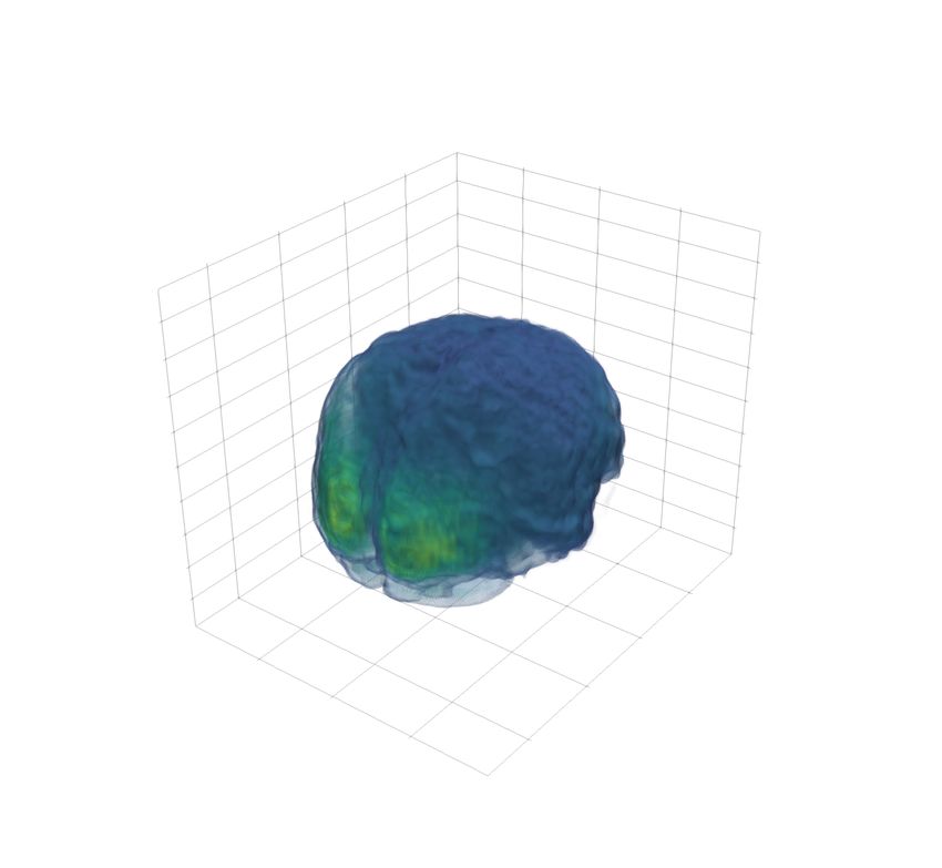
(a) fMRI images (b) fMRI volume (c) Cubical complex (d) Persistence diagrams (e) Persistence images
Figure 1: A graphical overview of our method. We represent an fMRI stack (a) as a volume (b),
from which we create a sequence of cubical complexes (c). Calculating the persistent homology of
this sequence results in a set of time-varying persistence diagrams (d); note that we only show the
diagrams for a single dimension of the cubical complex. We calculate summary statistics from the
diagrams (not shown), and convert them to vectorial representations (e) for analysis tasks.
Traditional approaches largely ignore these factors, considering them inevitable noise in the mea-
surements. Voxel activity is often either directly compared across different cognitive tasks, or the
time-varying activity of voxels in pre-defined brain regions sharing functional properties is correlated
to create a ‘functional connectivity’ graph. Our approach differs from existing approaches for fMRI
data analysis in two crucial ways, namely (i) it is coordinate-free, providing a stable representation
of high-level brain activity, even without a voxel-by-voxel match, and (ii) it does not require the
creation of a correlation graph, or operate on any other approximated graph structure (in contrast
to the M APPER algorithm [48], for example). Instead, our method uses the ‘raw’ voxel activations
themselves as a cubical complex, which we further characterise using time-varying persistence
diagrams that indicate the presences of topological features such as voids of various dimensions in the
voxel activations. These topological features are naturally invariant to a variety of shifts and noise (see
Section 4). Our formulation enables the non-parametric analysis of fMRI data both statically and
dynamically, i.e. for assessing differences between cohorts across time, and enabling insights into
time-varying topological brain state trajectories within cohorts or individuals. For individuals, we
use an averaged summary statistic over time that can be embedded to explore population structure
and variability statically, which we use to organise subjects in our test set by age. Then, after
clustering subjects into cohorts, we propose a novel method for producing a time-varying trajectory
of persistence diagrams that can be used to quantify the progression and entropy of brain states. In
summary, we make the following contributions:
• We present a novel non-parametric framework for transforming time-varying fMRI data into
time-varying topological representations.
• We empirically show that these representations (a) capture age-related differences, and
(b) shed light on the cognitive processes of age-stratified cohorts.
• Finally, we show that our topological features are more informative for an age prediction
task than other representations of the data set.
2 Background on topological data analysis
Topological data analysis (TDA) recently started gaining traction in machine learning [11, 25–
28, 30, 33, 38, 40, 41, 43, 59]. TDA is a rapidly-growing field that provides tools for analysing the
shape of data sets. This section provides a brief overview, aiming primarily for intuition and less
for depth (see also Section A.1 for a worked example). We refer to Edelsbrunner and Harer [20] for
details. To our knowledge, this is the first time that TDA has been directly applied to fMRI data (as
opposed to applying it on auxiliary representations such as functional connectivity networks).
Simplicial homology. The central object in algebraic topology is a simplicial complex K, i.e. a
high-dimensional generalisation of a graph, containing simplices of varying dimensions: vertices,
edges, triangles, tetrahedra, and their higher-dimensional counterparts. A graph, for example, can
be seen as a 1-dimensional simplicial complex, containing vertices and edges. Such complexes are
primarily used to describe topological objects such as manifolds1 . Simplicial homology refers to a
1
We deviate from this notion in this paper but follow the conventional exposition, which focuses primarily on
a simplicial view.
2
framework for analysing the connectivity of K via matrix reduction algorithms, assigning K a graded
set of mathematical groups, the homology groups. Homology groups describe the topological features
of K; in low dimensions d, these features are called connected components (d = 0), tunnels (d = 1),
and voids (d = 2), respectively. The number of d-dimensional topological features is referred to as
the dth Betti number βd ∈ N; it is used to distinguish between different topological objects: for
example, a circle (i.e. the boundary of a disk) has Betti numbers (1, 1) because there is a single
connected component and a single tunnel, while a filled square has Betti numbers (1, 0).

Persistent homology. The analysis of real-world data sets, having no preferred scale at which
features occur, requires a different approach: Betti numbers cannot be directly used here because
they only represent counts, i.e. a single scale. Endowing them with additional information leads to
persistent homology, an extension of simplicial homology that requires a simplicial complex K and
an additional function f : K → R, such as an activation function. If f only attains a finite set of
function values f0 ≤ f1 ≤ · · · ≤ . . . fm−1 ≤ fm , one can sort K according to them, leading to a
filtration—a nested sequence of simplicial complexes
                             ∅ = K0 ⊆ K1 ⊆ · · · ⊆ Km−1 ⊆ Km = K,                                     (1)
with Ki := {σ ∈ K | f (σ) ≤ fi }. Filtrations represent the evolution of K along f . Similar to the
Watershed transform in image processing [42], topological features can be created (a new connected
component might arise) or destroyed (two connected components might merge into one) in a filtration.
Persistent homology efficiently tracks topological features across a filtration, representing each one
of them as a tuple (fi , fj ) ∈ R2 , with i ≤ j and fi , fj ∈ im(f ).

Persistence diagrams. The tuples (fi , fj ) are collected according to their dimension d and stored
in the dth persistence diagram Dd , which summarises all d-dimensional topological activity. As a
consequence of the calculation process, all points in Dd are situated above the diagonal. The quantity
pers(x, y) := |y − x|, i.e. the distance to the diagonal (up to a constant factor), of a point (x, y) ∈ Dd
is called the persistence of its corresponding topological feature. Low-persistence features used to be
considered ‘noise‘, while high-persistence features are assumed to correspond to ‘real’ features of a
data set [21]. Recent work cast some doubts as to whether this assumption is justified [9]; in medical
data, low persistence merely implies ‘low reliability’, not necessarily ‘low importance’.

3   Related work
For fMRI analysis, the typical approach is to compare voxel activations directly, but when one is
interested in time-varying activity from a continuous stimulus (e.g. while watching a movie or resting),
voxel data is sometimes transformed into correlation matrices, either calculated across time points [4]
or across voxels [57] (studying functional connectivity, i.e. information about the connectivity between
brain regions sharing certain functional properties). Due to the size of the matrices in the latter
case, one also often reduces the dimensionality by applying an atlas parcellation [47]. Both of these
representations are efficacious, with voxel-by-voxel correlation matrices providing insights into the
topology and dynamics of human brain networks [52]. Moreover, for many multi-subject fMRI
studies, shared response models [13], abbreviated as SRMs, have proven effective. SRMs ‘learn’ a
mapping of multiple subjects into the same space, enabling the detection of group differences, or
the study of relations between brain activity and movie annotations, for example [54]. Recently,
SRM was used to map voxel activity into a functional space (as opposed to an anatomical one), to
study the brain representation of, among others, visual and auditory information while receiving
naturalistic audiovisual stimuli [29]. Nonetheless, while SRM is one of the most powerful techniques
for extracting cognitively-relevant signals from fMRI data, there is still room for improvement.
Previous work fusing fMRI analysis and topological data analysis is either based on auxiliary (topo-
logical) representations [44, 49], such as the M APPER algorithm [48] which operates on graphs, and
requires numerous parameter choices, or it makes use of functional connectivity information (in-
formation about connectivity between brain regions sharing functional properties) and pre-defined
regions of interest [3, 22, 24, 45]. By contrast, our method operates directly on fMRI volumes,
requiring neither additional location information nor auxiliary representations. We will instead make
use of cubical complexes, for which we essentially replace triangles by squares and tetrahedra by
cubes (see Figure 1c and the subsequent section for details). Cubical complexes and their homology
are well-studied in algebraic topology, but their use in real-world applications used to be limited to

                                                    3
image segmentation [2]. This changed with the rise of persistent homology, which was extended to
the cubical setting [37, 51, 55], leading to cubical persistent homology [18, 34, 56].

4       A topology-based framework for fMRI data sets

In the following, we will be dealing with time-varying fMRI. By this, we mean that we are observing
an activation function f : V × T → R over a 3D bounded volume V ⊂ R3 and a set of time steps T .
The alignment of V across different subjects is highly non-trivial; we provide more details about
this at the beginning of Section 5. For t ∈ T , the function f (·, t) is typically visualised using either
stacks of images (Figure 1a) or volume rendering (Figure 1b). While it would be possible to analyse
the topology of individual images [7], we want a holistic view of the topology of V. To this end, we
transform V into a cubical complex C, i.e. an equivalent of a simplicial complex, in which triangles
and tetrahedra are replaced by squares and cubes (see Figure 1c). Cubical complexes are perfectly
suited to represent an fMRI volume V because each voxel corresponds precisely to one cubical
simplex (whereas if we were to use a simplicial complex, we would have to employ interpolation
schemes as there is no natural mapping from voxels to tetrahedra; see Figure A.3 for more details).

Terminology. We assume that we are given a data set of n volumes V1 , . . . , Vn , corresponding to n
different individuals, and a set of m time steps T = {t1 , . . . , tm } ⊂ N. We use vert(Vi ) to denote
the vertex (i.e. voxel) set of Vi , and fi to denote its activation function, i.e. fi : Vi × T → R, Here,
the activation functions are aligned with respect to their time steps; this is an assumption that greatly
simplifies all subsequent analysis steps. It does not impose a large restriction in practice.

Topological features from fMRI data. We obtain topological features of each fi following a three-
step procedure, namely (1) cubical complex conversion, (2) filtration calculation, and (3) persistence
diagram calculation. The conversion of a volume Vi to a cubical complex Ci is simple, as Vi and
Ci share the same cubical elements and connectivities. Thus, the vertices of Ci are the voxels of Vi
and there are edges between neighbouring vertices as defined by a regular 3D grid, in which each
vertex has six neighbours (two per coordinate axis). These neighbourhoods implicitly define the
connectivity of higher-dimensional elements (squares and cubes). We will use σ to denote an element
of a cubical complex2 . Next, we impose a filtration—an ordering—of the elements of Ci . Since we
want to analyse topological features over time, we have to calculate a filtration for every time step.
Given tj ∈ T , we assign the values of fi (·, tj ) to Ci . We use the most natural assignment: each
vertex (voxel) of Ci receives its activation value at time tj , while a higher-dimensional element σ
is assigned a value recursively via fi (σ, tj ) := maxv∈vert(σ) fi (v, tj ). We then sort the cubical
complex Ci in ascending order according to these values; in case of a tie, a lower-dimensional
element (e.g. an edge) precedes a higher-dimensional one (e.g. a square). Having obtained a filtration
according to Equation 1, we may now calculate the persistent homology of Ci at time step tj ,
resulting
        in a collection of persistence
                                          diagrams. Since each Vi is three-dimensional, we obtain a
           (i,j)  (i,j)  (i,j)
triple D0 , D1 , D2              for every time step tj ; persistence diagrams for d ≥ 3 are all empty.
Notice that the calculation of persistence diagrams for a participant i and a time step tj can be easily
parallelised, since we treat time steps independently. Subsequently, we will use D(i) to denote the set
of all persistence diagrams associated with the ith participant. We can plot the resulting persistence
diagrams of each participant as a set of diagrams in R3 , with the additional axis being used to
represent time (Figure 1d).
The filtration that we employ here is also known as a sublevel set filtration. Other filtrations could
also be used (our method is not restricted to any specific one), but a symmetry theorem [16] states
that, unless we are willing to modify the activation function values themselves, we are not gaining
any more information about the topology of our input data. For the subsequent analyses, we will be
dealing with collections of persistence diagrams D(i) . The space of persistence diagrams affords
several metrics [15, 17], but they are computationally expensive and infeasible for the cardinalities
we are dealing with (a typical persistence diagram of a participant contains about 10000 features).
We will thus be working with topological summary statistics and persistence diagram vectorisations.

    2
     These elements are the ‘simplices’ of the cubical complex, but we refrain from re-using the term ‘simplex’
so as not to confuse ourselves or the reader.

                                                      4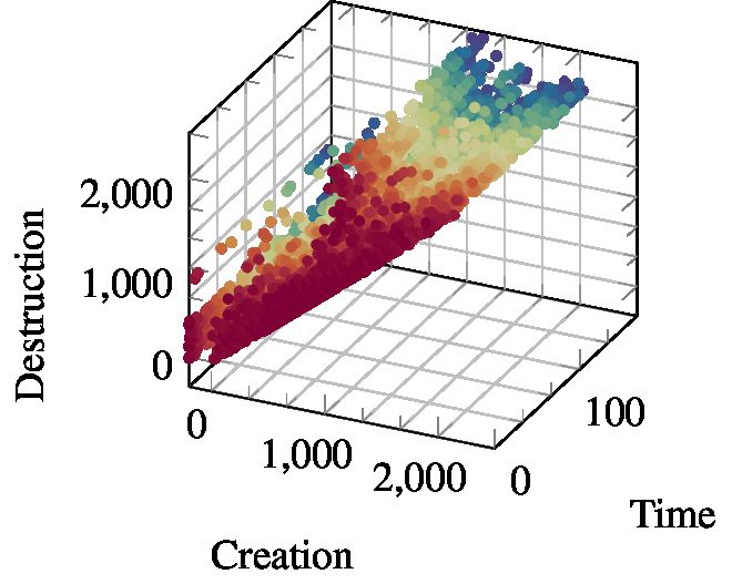
Properties. Prior to delving deeper into our pipeline, we describe some properties of our approach
and why topological features are advantageous. Topology is inherently coordinate-free, meaning that
all the features we describe are invariant to homeomorphism, i.e. stretching and bending. Moreover,
the persistence diagrams of spaces of different cardinalities and scales can be compared, making it
possible to ‘mix’ participants from studies with different imaging modalities or resolutions (of course,
this should not be done indiscriminately). Arguably the largest advantage of persistent homology is
its stability with respect to perturbations. This is quantified by the following theorem, whose proof
we defer to Section A.6.
Theorem 1. Let f : V → R and g : V → R be two activation functions. Then their corre-
sponding persistence diagrams Df and Dg satisfy W∞ (Df , Dg ) ≤ kf − gk∞ , where W∞ de-
notes the bottleneck distance between persistence diagrams [15], defined as W∞ (Df , Dg ) :=
inf η : D→Dg supx∈Df kx − η(x)k∞ , with η : Df → Dg denoting a bijection between the points of
the two diagrams, and k · k∞ referring to the L∞ norm.

The consequence of this stability theorem is that the persistence diagrams that we calculate are
 stable with respect to perturbations, provided those perturbations are of small amplitudes. This is a
 desirable characteristic for a feature descriptor because it provides us with well-defined bounds for
 its behaviour under noise. A more precise version of this stability theorem exists [17], but requires
 a more involved setup3 , which we leave for future work. In general, we note that time-varying
TDA is still a rather nascent sub-field of TDA. A standard approach, namely the calculation of
‘persistence vineyards’ [14], resulting in a decomposition of a time-varying persistence diagram into
 individual ‘vines’, is not applicable here because the changes between different time steps are not
 infinitesimal (there is a large amount of temporal coherence between consecutive time steps, but there
 is no guarantee that the change between them is upper-bounded). It is still unknown in our setting
whether a vineyard representation with unique vines exists at all [35]. We therefore prefer to treat the
 individual time steps as independent calculations but note that future work should address a more
 efficient computation by exploiting similarities between consecutive time steps.

Implementation and complexity. While the general calculation of persistent homology on high-
dimensional simplicial complexes is still computationally expensive, there are highly-efficient algo-
rithms for lower-dimensional calculations [6]. Here, we use DIPHA [5], a distributed implementation
of persistent homology, as it implements an efficient algorithm for computing topological features
of cubical complexes [55]. Space and time complexity is linear in the number of voxels, so our
conversion process does not change the complexity of processing the data. The persistent homology
calculation has a time complexity of O(|V|)ω , with ω ≈ 2.376 [31]. The distributed implementation
of DIPHA is reported [5] to be capable of calculating persistent homology for |V| ≈ 109 , making
our pipeline feasible and scalable. For the persistence image calculation in Section 5.2, we use
Scikit-TDA [46]. We make our code available to ensure reproducibility.

5       Results
We evaluate our topological pipeline using open-source fMRI data [39], available on the OpenNeuro
database (accession number ds000228). The participants comprised 33 adults (18–39 years old; M
= 24.8, SD = 5.3; 20 female) and 122 children (3.5–12 years old; M = 6.7, SD = 2.3; 64 female)
who watched the same animated movie ‘Partly Cloudy’ [50] while undergoing fMRI. Please refer to
Section A.3 and Yates et al. [58] for a full description of the pre-processing. The relevant outputs of
these pre-processing steps are: a 4-dimensional (x × y × z × t, with x, y, z being coordinates, and t
representing time) fMRI time series and a whole-brain mask (BM) for each individual subject. The
fMRI time series includes 168 time steps (each comprising 2 s of the movie) that correspond to the
same point in the movie for each subject; since for the first five time steps only a blank screen was
shown, we remove these plus two time steps to account for the fMRI hemodynamic lag for all analyses.
We supplemented the whole-brain mask by also creating an ‘occipital-temporal’ mask (OM) for each
subject. This entailed finding the intersection between an individual subject’s whole-brain mask and
occipital, temporal, and precuneus regions of interest defined from the Harvard–Oxford cortical atlas.
If our results reflect patterns relevant to cognitive processing, we would expect similar—if not better
results—using this occipital-temporal mask, since it contains the regions most consistently involved
    3
        We will have to show Lipschitz continuity for the functions, plus certain other properties of the space V.

                                                          5
1,500
1,400
1,300
1,200 kDk∞
340,000
320,000
300,000
kDk1
280,000
50 100 150
(a) Persistence diagrams (b) Persistence diagram (c) Summary statistics
Figure 2: Example of summary statistics calculations. Starting from a sequence of time-varying
persistence diagrams (a) of one participant, for each diagram slice (b), we evaluate a scalar-valued
statistic S : D → R, leading to a time series (c); the corresponding time point is highlighted.
Method BM OM XM
BASELINE - TT 0.09 0.02 0.24
BASELINE - PP 0.41 0.40 0.40
SRM 0.44 — —
kDk1 0.46 0.67 0.48
kDk∞ 0.61 0.77 0.73
(a) BASELINE - TT (b) BASELINE - PP (c) kDk1 (d) kDk∞ (e) Age prediction task
Figure 3: An embedding of the distances for different baselines and topological summaries, based on
the whole-brain mask (BM); colour-coding refers to the age group of participants. The table depicts
the results of the age prediction task, stratified by different brain masks; performance is measured as
a correlation coefficient (bold indicates the best results).
in movie-watching (e.g. visual regions). Last, we also calculated the ‘logical XOR’ between the
whole-brain mask and the occipital-temporal mask; this mask (XM) makes it possible to study the
relevance of topological features with respect to non-visual regions (including the frontal lobe) in
the brain. To prevent analysis bias, data were initially fully unlabelled during the development of
our pipeline. Later on, participants were assigned to cohorts based on their age group, using the
same bins as Yates et al. [58]; we initially did not know whether cohorts were sorted in ascending
or descending order. The actual ages were only used in the age prediction experiment, which was
performed after method development had ceased.
5.1 Static analysis based on summary statistics
Extracting information from the time-varying persistence diagrams of each participant is impeded by
their complex geometrical structure, making it necessary to use summary statistics. We first focus on
a description of global properties of participants, restricting ourselves to persistence diagrams with
d = 2 (i.e. we are studying voids of the activation function). To this end, we calculate topological
summary statistics of the form S : D → R. We calculate two related summary statistics here, namely
the infinity norm kDk∞ of a persistence diagram [15] and the p-norm4 kDkp [12, 17], defined by
s X
kDk∞ := max pers(x, y)p and kDkp := p pers(x, y)p , (2)
x,y∈D
x,y∈D
with p ∈ R. We found p = 1 to be sufficient (thus using unscaled persistence values). Since
Equation 2 results in a single scalar value for a persistence diagram, the summary statistics turn a
sequence of time-varying persistence diagrams into a time series of scalar-valued summary statistics.
Figure 2 depicts this for a single participant of our data.
Qualitative evaluation. Figure 3 shows an embedding obtained from our topological summary
statistics (using multidimensional scaling based on the Euclidean distance between per-participant
curves) compared to baseline embeddings, which we obtain from the two correlation matrices
described in Section 3. We refer to them as BASELINE - TT (time-based) and BASELINE - PP (voxel-
based; parcellated for computational ease), respectively (see Section A.4 for additional details). Both
4
The term total persistence is sometimes used interchangeably for this norm.
6topology-based embeddings are showing a split between participants. By colour-coding the age group
of each participant, we see that topology-based embeddings separate adults (red) from children (other
colours). The baselines, by contrast, do not exhibit such a clear-cut distinction.
Quantitative evaluation. To quantify the benefits of our proposed topological feature extraction
pipeline, we set up a task in which we predict the age of the non-adult participants. Using a ridge
regression and leave-one-out cross-validation (see Section A.5 for additional experimental details),
we train models on either the curves of summary statistics (not the embeddings) or the baseline
matrices, reporting the correlation coefficient in the table in Figure 3. Higher values indicate that the
model is better suitable to predict the age. The SRM result comes from previous work on the same
data set [58]; we note that our task is slightly different5 . Overall, we observe strong correlations,
indicating that topological features are highly useful for age prediction and carry salient information.
Performance based on the occipital-temporal mask (OM) and on the XOR mask (XM) is higher than
for the whole-brain mask (BM); we hypothesise that this partially due to the higher noise level of
BM, whereas OM and XM focus only on a subset of the brain (which decreases the noise level). We
also note that kDk∞ , which only considers the most persistence topological feature of a persistence
diagram, performs best in the prediction task, possibly because it is more robust to small-scale noise
5.2 Dynamic analysis based on brain state trajectories
So far, we dealt only with overall summary statistics. Our framework also enables analysing
the brain state of participants over time. We sidestep the aforementioned issue of persistence
diagram metric computations by calculating persistence images [1] from the persistence diagrams.
A
Ppersistence image is a function Ψ : R → R that turns a diagram D into a surface via Ψ(z) :=
2
x,y∈D w(x, y)Φ(x, y, z), where w(·) is a fixed piecewise linear weight function and Φ(·) denotes
a probability distribution, which is typically chosen to be a normalised symmetric Gaussian. By
discretising Ψ (using an r × r grid), a persistence diagram is transformed into an image6 ; this is
depicted in Figure 1e. The main advantage of Ψ lies in embedding persistence diagrams into a space
that is amenable to standard machine learning tools; moreover, Ψ affords defining and calculating
unique means, as opposed to persistence diagrams [35, 36, 53]. Subsequently, we use r = 20 and a
Gaussian kernel with σ = 1.0; Ψ is known to be impervious to such choices [1].
5.2.1 Cohort brain state trajectories
(i,j)
By evaluating Ψ(D2 ) for each time step tj , we turn the sequence of persistence diagrams of
2
the ith participant into a matrix X(i) ∈ Rm×r , where the jth row corresponds to the ‘unravelled’
persistence image of time step tj . We now calculate the sample mean Xk of each participant cohort,
resulting in six matrices whose rows represent the average topological activity of participants in the
respective cohort. Taking the Euclidean distance between persistence images as a proxy for their
actual topological dissimilarity [1, Theorem 3], we calculate pairwise distances between rows of each
Xk and embed them using PHATE [32], a powerful embedding algorithm for time-varying data. This
turns Xk into a 2D brain state trajectory (where the state is measured using topological features).
Figure 4 depicts the resulting trajectories for different masks. All brain state trajectories exhibit
visually distinct behaviour in older and younger subjects. The youngest subjects are characterised by
a simple ‘linear’ trajectory in the whole-brain mask, indicating that their processing of the movie
is more sensory-driven. This pattern is visible in Figure 4b for young children in general: until
7.5 yr, sensory processing, analysed using the occipital-temporal mask, is comparatively simple. In
older subjects, we observe more complex trajectories with higher entropy generally. Developmental
differences are best indicated in Figure 4c, where we see that the overall trajectory shape becomes
‘adult-like’ earlier (and thus more complex). Since this mask is composed of more cognitive brain
regions (rather than sensory ones), we hypothesise that this could indicate that older participants—
including older children—are capable of connecting different aspects of the movie to their memories,
for example, whereas the simpler trajectories of the two youngest cohorts in all brain masks may
indicate that these participants are not comprehending the movie on a non-superficial level.
5
Yates et al. [58] learn a shared set of features in adult participants to predict the age of non-adults.
6
Intuitively, this can also be seen as a form of kernel density estimation on persistence diagrams.
70.2
Average variability
0.1
0
-3 -2 -1 0 1 2 3
3.5–4.5yr 4.5–5.5yr 5.5–7.5yr 7.5–9.5yr 9.5–12.3yr 18–39yr Time steps to event boundary
(a) Whole-brain mask (entropy: 0.61, 0.97, 1.73, 1.15, 1.30, 1.67)
0.2
Average variability
0.1
0
-3 -2 -1 0 1 2 3
3.5–4.5yr 4.5–5.5yr 5.5–7.5yr 7.5–9.5yr 9.5–12.3yr 18–39yr Time steps to event boundary
(b) Occipital-temporal mask (entropy: 0.87, 0.65, 1.03, 0.94, 0.82, 1.46)
0.2
Average variability
0.1
0
-3 -2 -1 0 1 2 3
3.5–4.5yr 4.5–5.5yr 5.5–7.5yr 7.5–9.5yr 9.5–12.3yr 18–39yr Time steps to event boundary
(c) XOR mask (entropy: 0.86, 0.85, 1.13, 0.60, 0.88, 0.87)
Figure 4: Cohort brain state trajectories for different masks. Annotations provide the age range of
subjects in one cohort. Variability histograms are shown as the rightmost plot;their x-axis shows
the time steps prior (negative) or after (positive) an event boundary, while their y-axis depicts
across-cohort variability (please refer to Section 5.2.2 for more details);
5.2.2 Variability analysis
To quantify the variability across cohorts, we calculate the per-column maximum of each Xk ,
referring to the respective set of values as kXk k∞ ∈ Rm ; the calculated values are the equivalent
of the infinity norm evaluated (per time step) on a mean persistence image of the cohort. We finally
calculate s kX1 k∞ , . . . , |X6 k∞ , i.e. the sample standard deviation per time point, thus obtaining a
variability curve of m time steps (see Figure A.5). To use this variability curve, we ran an online
study to discover which salient events are detected by participants in the movie. Using 22 test
subjects (with no overlap to the ones used in the fMRI data acquisition process), we followed Ben-
Yakov and Henson [8] and determined consensus boundaries of events in the movie. We declare
an event boundary to be salient if at least 7 participants agree, resulting in 20 events. Given this
information, we collect the average variability over all events for a window of w = 3 time steps before
and after an event, leading to averaged variabilities {s1 , . . . , s7 }, where s4 corresponds to average
variability at the event boundary itself (see histograms in Figure 4). It is our hypothesis that post-event
and pre-event variability are different—in other words, our topological features capture cognitive
differences across cohorts and events. To quantify this, we calculate spre := maxi≤3 si − mini≤3 si
and spost := maxi≥5 si − mini≥5 si . We set θ := spre − spost as our test statistic and perform a
bootstrap procedure by sampling 20 time points at random and repeating the same calculation, thereby
obtaining an empirical null distribution. This results in bootstrap samples θb1 , . . . , θb1000 serving as a
null distribution θ,
b from which we obtain the achieved significance level (ASL) as Pr(θb ≥ θ).
The ASL values are 0.084 (whole-brain mask, BM), 0.045 (occipital-temporal mask, OM), and
0.396 (XOR mask, XM), respectively, indicating that the effect of capturing events is strongest in
OM (and significant at the α = 0.05 level). This aligns well with the gradual differences between
cohorts expressed in Figure 4b. Event differences are less pronounced in BM (which, as Figure 4a
shows, is capturing more complex cohort patterns). Finally, event differences are absent in XM,
showing that across-cohort variability is not consistent with event boundaries here, hinting at the
fact that this mask might better be used to assess within-cohort variability rather than across-cohort
variability. Please refer to Section A.7 for additional visualisations.
86 Conclusion
This paper demonstrates the potential of an unsupervised, non-parametric topology-based feature
extraction framework for fMRI data, permitting both static and dynamic analyses. We showed that
topological summary statistics are useful in an age prediction task. Using vectorised topological
features descriptors, we also developed cohort brain state trajectories that show the time-varying
behaviour of a cohort of participants (binned by age). Next, to highlight qualitative age-related differ-
ences in the overall cognition of participants, we were also able to uncover quantitative differences in
event processing. In the future, we want to further analyse the geometry of brain state trajectories
and link states back to events; a preliminary analysis (see Section A.8) finds significant differences
between the mean curvature [19] of adult and non-adult participants, thus showcasing the explanatory
potential of topological features.
Broader impact
The primary contribution of this work—a novel, parameter-free way of extracting informative features
from fMRI data—is of a computational nature. In general, we fully acknowledge that any researcher
dealing with fMRI data analysis (not necessarily restricted to machine learning methods) has a big
responsibility. Since our work is purely computational, we do not believe that it will have adverse
ethical consequences, provided the experimental design is unbiased. For the same reason, our work is
not specifically favouring or disfavouring any groups.
Beyond the immediate applications for fMRI data analysis, our work also has a broader applicability
for the analysis of time-varying or structured neuroscience data in general. This includes other
non-invasive techniques such as EEG or MEG, but also neuronal spike data from cell populations.
Our work is appealing for such data because it does not require auxiliary representations such as
graphs. We are thus convinced that the introduction of our directly-computable topological features
will overall have beneficial outcomes.
As long-term goal, for example, our work could serve as a foundation to investigate neurological
pathologies (such as depressive disorders) from a new, topological perspective. In general, our
dynamic analyses also allow us to capture not just stable traits in different populations, but also
the different mental states participants progress through while undergoing fMRI. As a generic
feature descriptor of brain states, we would welcome a future in which topological features aid in
understanding such traits or states.
References
[1] H. Adams, T. Emerson, M. Kirby, R. Neville, C. Peterson, P. Shipman, S. Chepushtanova, E. Hanson,
F. Motta, and L. Ziegelmeier. Persistence images: A stable vector representation of persistent homology.
Journal of Machine Learning Research, 18(8):1–35, 2017.
[2] M. Allili, K. Mischaikow, and A. Tannenbaum. Cubical homology and the topological classification of 2D
and 3D imagery. In Proceedings of the IEEE International Conference on Image Processing, volume 2,
pages 173–176, 2001.
[3] K. L. Anderson, J. S. Anderson, S. Palande, and B. Wang. Topological data analysis of functional MRI
connectivity in time and space domains. In Connectomics in NeuroImaging, 2018.
[4] C. Baldassano, J. Chen, A. Zadbood, J. W. Pillow, U. Hasson, and K. A. Norman. Discovering event
structure in continuous narrative perception and memory. Neuron, 95(3):709–721.e5, 2017.
[5] U. Bauer, M. Kerber, and J. Reininghaus. Distributed computation of persistent homology. In Proceedings
of the Meeting on Algorithm Engineering and Experiments (ALENEX), pages 31–38, 2014.
[6] U. Bauer, M. Kerber, J. Reininghaus, and H. Wagner. PHAT – Persistent Homology Algorithms Toolbox.
In H. Hong and C. Yap, editors, Mathematical Software – ICMS 2014, pages 137–143. Springer, 2014.
[7] P.-L. Bazin and D. L. Pham. Topology-preserving tissue classification of magnetic resonance brain images.
IEEE Transactions on Medical Imaging, 26(4):487–496, 2007.
[8] A. Ben-Yakov and R. N. Henson. The hippocampal film editor: Sensitivity and specificity to event
boundaries in continuous experience. Journal of Neuroscience, 38(47):10057–10068, 2018.
9[9] P. Bendich, J. S. Marron, E. Miller, A. Pieloch, and S. Skwerer. Persistent homology analysis of brain
artery trees. Annals of Applied Statistics, 10(1):198–218, 2016.
[10] L. Buitinck, G. Louppe, M. Blondel, F. Pedregosa, A. Mueller, O. Grisel, V. Niculae, P. Prettenhofer,
A. Gramfort, J. Grobler, R. Layton, J. VanderPlas, A. Joly, B. Holt, and G. Varoquaux. API design for
machine learning software: experiences from the scikit-learn project. In ECML PKDD Workshop:
Languages for Data Mining and Machine Learning, pages 108–122, 2013.
[11] M. Carrière, F. Chazal, Y. Ike, T. Lacombe, M. Royer, and Y. Umeda. PersLay: A neural network layer for
persistence diagrams and new graph topological signatures. arXiv e-prints, art. arXiv:1904.09378, 2019.
[12] C. Chen and H. Edelsbrunner. Diffusion runs low on persistence fast. In Proceedings of the IEEE
International Conference on Computer Vision, pages 423–430, 2011.
[13] P.-H. Chen, J. Chen, Y. Yeshurun, U. Hasson, J. Haxby, and P. J. Ramadge. A reduced-dimension fMRI
shared response model. In C. Cortes, N. D. Lawrence, D. D. Lee, M. Sugiyama, and R. Garnett, editors,
Advances in Neural Information Processing Systems 28, pages 460–468. Curran Associates, Inc., 2015.
[14] D. Cohen-Steiner, H. Edelsbrunner, and D. Morozov. Vines and vineyards by updating persistence in linear
time. In Proceedings of the 22nd Annual Symposium on Computational Geometry, pages 119–126, 2006.
[15] D. Cohen-Steiner, H. Edelsbrunner, and J. Harer. Stability of persistence diagrams. Discrete & Computa-
tional Geometry, 37(1):103–120, 2007.
[16] D. Cohen-Steiner, H. Edelsbrunner, and J. Harer. Extending persistence using Poincaré and Lefschetz
duality. Foundations of Computational Mathematics, 9(1):79–103, 2009.
[17] D. Cohen-Steiner, H. Edelsbrunner, J. Harer, and Y. Mileyko. Lipschitz functions have Lp -stable persistence.
Foundations of Computational Mathematics, 10(2):127–139, 2010.
[18] P. Dłotko and T. Wanner. Rigorous cubical approximation and persistent homology of continuous functions.
Computers & Mathematics with Applications, 75(5):1648–1666, 2018.
[19] M. P. do Carmo. Differential Geometry of Curves and Surfaces. Prentice-Hall, Inc., 1976.
[20] H. Edelsbrunner and J. Harer. Computational topology: An introduction. American Mathematical Society,
2010.
[21] H. Edelsbrunner, D. Letscher, and A. J. Zomorodian. Topological persistence and simplification. Discrete
& Computational Geometry, 28(4):511–533, 2002.
[22] C. T. Ellis, M. Lesnick, G. Henselman-Petrusek, B. Keller, and J. D. Cohen. Feasibility of topological data
analysis for event-related fMRI. Network Neuroscience, 3(3):695–706, 2019.
[23] O. Esteban, C. J. Markiewicz, R. W. Blair, C. A. Moodie, A. I. Isik, A. Erramuzpe, J. D. Kent, M. Goncalves,
E. DuPre, M. Snyder, H. Oya, S. S. Ghosh, J. Wright, J. Durnez, R. A. Poldrack, and K. J. Gorgolewski.
fMRIPrep: a robust preprocessing pipeline for functional MRI. Nature Methods, 16(1):111–116, 2019.
[24] C. Giusti, R. Ghrist, and D. S. Bassett. Two’s company, three (or more) is a simplex. Journal of
Computational Neuroscience, 41(1):1–14, 2016.
[25] C. Hofer, R. Kwitt, M. Niethammer, and A. Uhl. Deep learning with topological signatures. In I. Guyon,
U. V. Luxburg, S. Bengio, H. Wallach, R. Fergus, S. Vishwanathan, and R. Garnett, editors, Advances in
Neural Information Processing Systems 30, pages 1634–1644. Curran Associates, Inc., 2017.
[26] C. Hofer, R. Kwitt, M. Niethammer, and M. Dixit. Connectivity-optimized representation learning via
persistent homology. In K. Chaudhuri and R. Salakhutdinov, editors, Proceedings of the 36th International
Conference on Machine Learning (ICML), number 97 in Proceedings of Machine Learning Research,
pages 2751–2760. PMLR, 2019.
[27] X. Hu, F. Li, D. Samaras, and C. Chen. Topology-preserving deep image segmentation. In H. Wallach,
H. Larochelle, A. Beygelzimer, F. d’Alché-Buc, E. Fox, and R. Garnett, editors, Advances in Neural
Information Processing Systems 32, pages 5657–5668. Curran Associates, Inc., 2019.
[28] V. Khrulkov and I. Oseledets. Geometry score: A method for comparing generative adversarial net-
works. In J. Dy and A. Krause, editors, Proceedings of the 35th International Conference on Machine
Learning (ICML), number 80 in Proceedings of Machine Learning Research, pages 2621–2629. PMLR,
2018.
10[29] S. Kumar, C. T. Ellis, T. O’Connell, M. M. Chun, and N. B. Turk-Browne. Searching through functional
space reveals distributed visual, auditory, and semantic coding in the human brain. bioRxiv, 2020. doi:
10.1101/2020.04.20.052175.
[30] R. Kwitt, S. Huber, M. Niethammer, W. Lin, and U. Bauer. Statistical topological data analysis — a kernel
perspective. In C. Cortes, N. D. Lawrence, D. D. Lee, M. Sugiyama, and R. Garnett, editors, Advances in
Neural Information Processing Systems 28, pages 3070–3078. Curran Associates, Inc., 2015.
[31] N. Milosavljević, D. Morozov, and P. Skraba. Zigzag persistent homology in matrix multiplication time.
In Proceedings of the 27th Annual Symposium on Computational Geometry, pages 216–225, 2011.
[32] K. R. Moon, D. van Dijk, Z. Wang, S. Gigante, D. B. Burkhardt, W. S. Chen, K. Yim, A. v. d. Elzen, M. J.
Hirn, R. R. Coifman, N. B. Ivanova, G. Wolf, and S. Krishnaswamy. Visualizing structure and transitions
in high-dimensional biological data. Nature Biotechnology, 37(12):1482–1492, 2019.
[33] M. Moor, M. Horn, B. Rieck, and K. Borgwardt. Topological autoencoders. arXiv e-prints, art.
arXiv:1906.00722, 2019.
[34] M. Mrozek and T. Wanner. Coreduction homology algorithm for inclusions and persistent homology.
Computers & Mathematics with Applications, 60(10):2812–2833, 2010.
[35] E. Munch. Applications of Persistent Homology to Time Varying Systems. PhD thesis, Duke University,
2013.
[36] E. Munch, K. Turner, P. Bendich, S. Mukherjee, J. Mattingly, and J. Harer. Probabilistic Fréchet means for
time varying persistence diagrams. Electronic Journal of Statistics, 9(1):1173–1204, 2015.
[37] V. Nanda. Discrete Morse Theory For Filtrations. PhD thesis, Rutgers University, 2012.
[38] K. N. Ramamurthy, K. Varshney, and K. Mody. Topological data analysis of decision boundaries with
application to model selection. In K. Chaudhuri and R. Salakhutdinov, editors, Proceedings of the 36th
International Conference on Machine Learning (ICML), number 97 in Proceedings of Machine Learning
Research, pages 5351–5360. PMLR, 2019.
[39] H. Richardson, G. Lisandrelli, A. Riobueno-Naylor, and R. Saxe. Development of the social brain from
age three to twelve years. Nature Communications, 9(1):1–12, 2018.
[40] B. Rieck, C. Bock, and K. Borgwardt. A persistent Weisfeiler–Lehman procedure for graph classification.
In K. Chaudhuri and R. Salakhutdinov, editors, Proceedings of the 36th International Conference on
Machine Learning, volume 97 of Proceedings of Machine Learning Research, pages 5448–5458. PMLR,
2019.
[41] B. Rieck, M. Togninalli, C. Bock, M. Moor, M. Horn, T. Gumbsch, and K. Borgwardt. Neural persistence:
A complexity measure for deep neural networks using algebraic topology. In International Conference on
Learning Representations (ICLR), 2019.
[42] J. B. T. M. Roerdink and A. Meijster. The watershed transform: Definitions, algorithms and parallelization
strategies. Fundamenta Informaticae, 41:187–228, 2000.
[43] M. Royer, F. Chazal, C. Levrard, Y. Ike, and Y. Umeda. ATOL: Measure vectorisation for automatic
topologically-oriented learning. arXiv e-prints, art. arXiv:1909.13472, 2019.
[44] M. Saggar, O. Sporns, J. Gonzalez-Castillo, P. A. Bandettini, G. Carlsson, G. Glover, and A. L. Reiss.
Towards a new approach to reveal dynamical organization of the brain using topological data analysis.
Nature Communications, 9(1):1399, 2018.
[45] F. A. N. Santos, E. P. Raposo, M. D. Coutinho-Filho, M. Copelli, C. J. Stam, and L. Douw. Topological
phase transitions in functional brain networks. Physical Review E, 100:032414, 2019.
[46] N. Saul and C. Tralie. Scikit-TDA: Topological data analysis for Python, 2019. URL https://doi.
org/10.5281/zenodo.2533369.
[47] A. Schaefer, R. Kong, E. M. Gordon, T. O. Laumann, X.-N. Zuo, A. J. Holmes, S. B. Eickhoff, and B. T. T.
Yeo. Local–global parcellation of the human cerebral cortex from intrinsic functional connectivity MRI.
Cerebral Cortex, 28(9):3095–3114, 2017.
[48] G. Singh, F. Mémoli, and G. Carlsson. Topological methods for the analysis of high dimensional data sets
and 3D object recognition. In Eurographics Symposium on Point-Based Graphics, 2007.
11[49] A. E. Sizemore, J. E. Phillips-Cremins, R. Ghrist, and D. S. Bassett. The importance of the whole:
Topological data analysis for the network neuroscientist. Network Neuroscience, 3(3):656–673, 2019.
[50] P. Sohn and K. Reher. Partly Cloudy [motion picture], 2009. Pixar Animation Studios and Walt Disney
Pictures.
[51] D. Strömbom. Persistent homology in the cubical setting: Theory, implementations and applications.
Master’s thesis, Luleå University of Technology, 2007.
[52] N. B. Turk-Browne. Functional interactions as big data in the human brain. Science, 342(6158):580–584,
2013.
[53] K. Turner, Y. Mileyko, S. Mukherjee, and J. Harer. Fréchet means for distributions of persistence diagrams.
Discrete & Computational Geometry, 52(1):44–70, 2014.
[54] K. Vodrahalli, P.-H. Chen, Y. Liang, C. Baldassano, J. Chen, E. Yong, C. Honey, U. Hasson, P. Ramadge,
K. A. Norman, and S. Arora. Mapping between fMRI responses to movies and their natural language
annotations. NeuroImage, 180:223–231, 2018.
[55] H. Wagner, C. Chen, and E. Vuçini. Efficient computation of persistent homology for cubical data.
In R. Peikert, H. Hauser, H. Carr, and R. Fuchs, editors, Topological Methods in Data Analysis and
Visualization II: Theory, Algorithms, and Applications, pages 91–106. Springer, 2012.
[56] B. Wang and G.-W. Wei. Object-oriented persistent homology. Journal of Computational Physics, 305:
276–299, 2016.
[57] Y. Wang, J. D. Cohen, K. Li, and N. B. Turk-Browne. Full correlation matrix analysis (FCMA): An
unbiased method for task-related functional connectivity. Journal of Neuroscience Methods, 251:108–119,
2015.
[58] T. S. Yates, C. T. Ellis, and N. B. Turk-Browne. Emergence and organization of adult brain function
throughout child development. bioRxiv, 2020. doi: 10.1101/2020.05.09.085860.
[59] Q. Zhao and Y. Wang. Learning metrics for persistence-based summaries and applications for graph
classification. In H. Wallach, H. Larochelle, A. Beygelzimer, F. d’Alché-Buc, E. Fox, and R. Garnett,
editors, Advances in Neural Information Processing Systems 32, pages 9855–9866. Curran Associates,
Inc., 2019.
12A Appendix
The following sections provide additional details about the experiments as well as a brief glimpse
into other analyses that we are actively pursuing for future work.
A.1 An intuitive introduction to persistent homology
Persistent homology was developed as a ‘shape descriptor’ for real-world data sets, where the
idealised notions of algebraic topology do not necessarily apply any more. This is illustrated by the
subsequent figure, which deals with a point cloud that has a roughly circular shape. Notice that this
shape is immediately recognisable to humans, but from the perspective of algebraic topology, it is
merely a collection of points with a trivial shape.
We observe that we can analyse this point cloud by picking an appropriate scale parameter. More
precisely, if we start connecting points that are within a certain distance to each other, we obtain a
nested sequence of simplicial complexes (in our context, this term is synonymous with a graph) as
we increase . This is a special type of filtration—a filtration based on pairwise distances, and the
resulting simplicial complexes are depicted above. It is now possible to calculate Betti numbers for
each of these complexes. Since we are only dealing with 2D points, there are only two relevant Betti
numbers, namely β0 and β1 , corresponding to the number of connected components and the number
of cycles, respectively. Suppose now that we track these numbers for each one of the steps in the
filtration; moreover, suppose we have a way of making the individual steps in the filtration as small
as possible such that we never miss any changes in β0 and β1 . For every topological feature—every
component and every cycle—we can thus measure precisely when a feature was created and when it
was destroyed.
Persistence diagram. This information is collected in the persistence diagram, which summarises
all topological activity. In this example, the persistence diagram of the 1-dimensional topological
features contains a few points, each one of them corresponding to one specific cycle in the data.
The axes correspond to the scale parameter (their actual values can
be safely ignored for this illustrative example). The x-axis shows the 1
threshold at which a cycle was created, i.e. at which there is a ‘hole’
in the corresponding simplicial complex, while the y-axis depicts 0.8
the threshold at which this hole is destroyed, i.e. closed. We do not 0.6
specifically indicate this here, but cycles are destroyed whenever all 0.4
points that are involved in their creation are connected to each other.
Put differently, this means that we ignore cycles created by individual 0.2
triangles of points, for example, as they are qualitatively different 0
from cycles created by arranging points in such a circular shape (there 0 0.2 0.4 0.6 0.8 1
are more technical reasons for this restriction). In any case, the
persistence diagram demonstrates that virtually all cycles—depicted A persistence diagram of
as points—occur at small scales, except for one. This coincides with the 1-dimensional topologi-
our intuition: we do not perceive such a point cloud to have a lot of cal features (cycles).
large-scale cycles. The persistence diagram thus serves as an intuitive
feature descriptor: points that occur at large scales are far removed from the diagonal (and have a
high persistence), whereas the small-scale features cluster around the diagonal.
The interesting fact is that knowing the persistence diagram also makes it possible for us to ‘guess’ the
number of relevant scales of a point cloud! In this example, we would possibly state that there is only
one useful scale at which to analyse the data, namely the scale for which the cycle structure becomes
topologically apparent. In general, this will differ based on the data set. Persistent homology does not
force us to prefer a scale, making it suitable for the analysis of real-world data sets. The ingenious
realisation of Edelsbrunner et al. [21] was that there is no reason to ‘guess’ scales or compute Betti
13numbers per step, as we described it above. Instead, it is possible to obtain information about all
potential scales by a single pass through the data, making this a highly-efficient algorithm (at least as
long as the dimension of the input data is bounded; calculating topological features for dimensions
d
3 efficiently is still a topic of ongoing research).
Persistence images. Since the metric structure of persistence diagrams is known to be complex [36],
various kernel-based and ‘vectorisation’ methods exist. In the main text, we focus on persistence
images [1], a technique that essentially estimates the density of a persistence diagram and uses a
grid to obtain a fixed-size representation. Such representations may then be used for downstream
processing tasks. As a worked example, consider the following persistence diagram. After rotating
it so that the diagonal becomes the new x-axis, we can perform density estimates with different
resolutions. The density estimator, which is by default a Gaussian kernel, can be adjusted as well,
but Adams et al. [1] mention that this does not have a large influence on the results (whereas the
resolution should be sufficiently large to capture differences). In the main paper, we use a smoothing
value of σ = 1 and a resolution of r = 20, resulting in 400-dimensional vectors. We also calculated
different resolutions and smoothing values, but the results are virtually identical, unless the resolution
is decreased too much: recall that a single persistence diagram of one participant has around 10000
features; reducing them to a, say, 5 × 5 image results in a large loss of information.
A.2 Properties of cubical complexes
Figure A.3 depicts the differences between cubical complexes and simplicial complexes. The cubical
complex is ‘aligned’ with a regular grid and does not force us to choose between an interpolation
scheme. For a simplicial complex, however, the calculation of topological features in dimensions 1
and 2 necessitates the creation of 2-simplices, i.e. triangles. This, in turn, requires us to ‘pick’
between two triangulation schemes that result in different connectivities between the original vertices.
In the worst case, this could lead to subtle differences in filtrations, since the new edges need to be
weighted accordingly.
A.3 fMRI pre-processing
The fMRI data acquisition used the following parameters: gradient-echo EPI sequence: TR = 2 s,
TE = 30 ms, flip angle = 90◦ , matrix = 64 × 64, slices = 32, interleaved slice acquisition. Data were
collected using the standard Siemens 32-channel head coil for adults and older children. One of two
custom 32-channel phased-array head coils was used for younger children (smallest coil: N = 3; M
= 3.91, SD = 0.42 years old; smaller coil: N = 28; M = 4.07, SD = 0.42, years old). Acquisition
parameters differed slightly across participants but all fMRI data were re-sampled to have the same
voxel size: 3 mm isotropic with 10% slice gap. A T1-weighted structural image was also collected
for all subjects (MPRAGE sequence: GRAPPA = 3, slices = 176, resolution = 1 mm isotropic, adult
coil FOV = 256 mm, child coils FOV = 192 mm). Imaging data were pre-processed using fMRIPrep
v1.1.8 [23].
A.4 Baselines
As additional comparison partners, we calculate a time point correlation matrix and a spatial correla-
tion matrix (see Section 3). These matrices are calculated from the time-varying fMRI data of a single
participant, which is a 4D tensor indexed by time steps and spatial coordinates. By ‘unravelling’ the
spatial dimensions of the tensor (using a row-major ordering, for example), the 4D tensor becomes
a 2D tensor, i.e. a matrix in which each row corresponds to a single time step, and the columns
correspond to voxels in the aforementioned order. From this m × N matrix, where m denotes the
14You can also read