Adding the molecular dynamics functionality to the quantum Monte Carlo code CASINO
←
→
Page content transcription
If your browser does not render page correctly, please read the page content below
Adding the molecular dynamics functionality to the quantum
               Monte Carlo code CASINO
                               Mike Towler1 , Norbert Nemec2
                                1
                                 Theory of Condensed Matter Group,
                            Cavendish Laboratory, Cambridge University,
                         J.J. Thomson Avenue, Cambridge CB3 0HE, U.K.
                           2
                             Department of Physics and Astronomy, UCL,
                              Gower Street, London WC1E 6BT, U.K.

                                      November 15, 2011

                                              Abstract
       This report describes developments to the CASINO Quantum Monte Carlo code for en-
   abling coupled Diffusion Monte Carlo (DMC) and Density Functional Theory (DFT) molecular
   dynamics simulations. The main objective of the work is to develop a scalable interface be-
   tween CASINO and the PWscf code (which is part of Quantum ESPRESSO). CASINO will
   be modified with an algorithm based on re-weighting, level-cross checking and periodic Jastrow
   recomputation. An interface will also be developed for the data communication and transfer
   between PWscf and CASINO. Following are the outcomes of the work:
      • The interface between PWscf and CASINO was developed and is now provided through a
        file with a standard format containing: geometry, basis set, and orbital coefficients.
      • To improve the parallel efficiency of the DMC algorithm, the allocation and re-distribution
        of walkers (i.e. the list of current electron positions and various associated quantities
        related to the energy and wave function) between the cores was optimised by implementing
        asynchronous communication to overlap computation.
      • The work on parallel efficiency significantly improved the behaviour of CASINO. For a
        fixed target of 100 per core for a total walker population, linear weak scalability has been
        demonstrated for over 80,000 cores on the Jaguar Cray XT5 machine (1.75 petaFLOPS)
        at Oak Ridge National Laboratory. Furthermore, with 82,944 cores, CASINO version
        2.7 is more than 30% faster than version 2.6 and the total cost of re-distributing walkers
        (including the DMC equilibration) was reduced from 412 seconds to 1 second. This means
        it will be possible to use CASINO on machines with more than 100,000 cores.
      • Further minor modifications were also made to the CASINO distribution including: mul-
        tiple pseudopotentials for elements with the same atomic number, support for running
        multiple jobs simultaneously, faster partial-ranking algorithm, interface support for CRYS-
        TAL09 and a major revision of the user manual.
   The developments have been introduced within the main CASINO (version 2.10) and PWscf
   (version 4.3) code bases.
dCSE Final Report: DMC-MD calculations in casino
N.Nemec and M.D. Towler
November 15, 2011
Contents
1 Note by MDT 2
2 Project overview 2
3 Formalities 3
3.1 Reweighting . . . . . . . . . . . . . . . . . . . . . . . . . . . . . . . . . . . . . . . . . 3
3.2 Reweighting efficiency . . . . . . . . . . . . . . . . . . . . . . . . . . . . . . . . . . . 3
3.3 Space warping . . . . . . . . . . . . . . . . . . . . . . . . . . . . . . . . . . . . . . . . 4
4 Usage 5
5 Case study: Silicon crystal 6
5.1 MD Without reweighting . . . . . . . . . . . . . . . . . . . . . . . . . . . . . . . . . 6
5.2 Amplitude of oscillations . . . . . . . . . . . . . . . . . . . . . . . . . . . . . . . . . . 8
5.3 SCF convergence . . . . . . . . . . . . . . . . . . . . . . . . . . . . . . . . . . . . . . 8
5.4 Reweighting demonstration . . . . . . . . . . . . . . . . . . . . . . . . . . . . . . . . 8
5.5 MD trajectory . . . . . . . . . . . . . . . . . . . . . . . . . . . . . . . . . . . . . . . 9
5.6 DMC MD calculation - single timestep with reweighting . . . . . . . . . . . . . . . . 10
5.7 Larger MD steps . . . . . . . . . . . . . . . . . . . . . . . . . . . . . . . . . . . . . . 11
5.8 Use space warping . . . . . . . . . . . . . . . . . . . . . . . . . . . . . . . . . . . . . 12
5.9 Without reweighting . . . . . . . . . . . . . . . . . . . . . . . . . . . . . . . . . . . . 13
5.10 Conclusions of these initial studies . . . . . . . . . . . . . . . . . . . . . . . . . . . . 13
6 Incorporation of the DMC-MD functionality into the CASINO distribution 14
6.1 CASINO support in PWSCF . . . . . . . . . . . . . . . . . . . . . . . . . . . . . . . 15
6.2 Pseudopotentials and their converters . . . . . . . . . . . . . . . . . . . . . . . . . . 17
16.3 The runpwscf script . . . . . . . . . . . . . . . . . . . . . . . . . . . . . . . . . . . . 17
6.4 The runqmcmd script . . . . . . . . . . . . . . . . . . . . . . . . . . . . . . . . . . . . 21
7 Other work 23
7.1 Full parallel efficiency on parallel computers . . . . . . . . . . . . . . . . . . . . . . . 23
7.1.1 Introduction . . . . . . . . . . . . . . . . . . . . . . . . . . . . . . . . . . . . 23
7.1.2 Other considerations for large parallel QMC computations . . . . . . . . . . . 30
7.1.3 Conclusions about QMC scaling on massively parallel machines . . . . . . . . 33
7.2 Additional improvements to the CASINO code . . . . . . . . . . . . . . . . . . . . . 33
1 Note by MDT
This project was abandoned halfway through by NN (who has now departed physics for new chal-
lenges) and the work was taken over by MDT some months later. This document is based on a
half-finished tex file discovered by MDT in the mass of files found in NN’s project directory - any
misunderstandings of the earlier work are the responsibility of MDT. Sections 1-5 were largely writ-
ten by NN (and retain his English usage, except where confusion would result); later sections were
written by MDT..
2 Project overview
Plan is to perform diffusion Monte Carlo (DMC) for molecular dynamic (MD) simulations following
the idea of Grossman and Mitas [1] of updating an existing population of DMC walkers to slightly
varying trial wave functions.
To this goal the necessary functionality in casino needs to be identified, implemented and tested
on test cases.
In its current (2010) form, the casino code allows continuing a DMC simulation with a population
of walkers saved from a previous run. Originally this functionality is designed for continuations on
an unchanged system. However, simply replacing the trial wave function file does work reasonably
well and directly reduces some of equilibration time.
The most straightforward way to implement the updating of the distribution of walkers is as follows
is by extending the routine that reads in the population from disk at the beginning of a continued
DMC run. From the user’s perspective, this results in the following process:
• start a new casino process for each MD time step
• consecutive MD time steps are run as continuations in casino. The config.out file written
by the previous MD step is renamed to config.in and read in as initial state for the following
MD step.
• A new flag dmc reweight configs activates a reweighting step after reading config.in
• A new flag dmc spacewarp configs activates space warping after reading config.in
2The implementation is planned in two stages:
I. Reweighting – the statistical weight of each walker is adjusted by the ratio between old and
new wave function absolute square value. Most of the necessary data is saved in config.out
already, the implementation extends an existing source fragment used for twist averaging.
II. Space warping – the ion positions need to be saved in config.in so that the continuation run
has access to both the old and the new ion positions. With this data available, space warping
itself can be implemented along with the reweighting loop.
3 Formalities
3.1 Reweighting
When the old trial wave function Ψ is replaced by a new (similar) wave function Ψ0 each walker
need to be reweighted as
0
0 Ψ (Ri ) 2
wi = wi ×
Ψ (Ri )
To preserve the total weight, a second step renormalizes the the individual walker weights as
P
00 0 Pj j
w
wi = wi 0
j wj
so that
X X
W 00 = wi00 = wi = W
i i
During this transition, the total energy of the current population is changed as
1 X 0 1 X 00 0
Etot = wi Eloc (Ri ) → Etot = wi Eloc (Ri )
W W
i i
The initial best estimate of the energy for the continuation run is obtained by shifting the old best
estimate by the energy shift of the current total energy:
0 0
Ebest = Ebest − Etot + Etot
Even if the old run had already resulted in a very good estimate Ebest , the initial value Ebest0
0 , so the averaging window for E
contains the full uncertainty of the reweighted total energy Etot best
needs to be reset similar to the beginning of a DMC run.
3.2 Reweighting efficiency
The reweighting process generally leads to a nearly correct but suboptimal distribution of walkers.
Set of N random variables with different weights wi , an effective sample size can be defined as:
P
( i wi ) 2
Neff = P 2
i wi
3(see also N. Nemec [2]).
For homogeneous weights, the effective sample size Neff equals the sample size N . When the
weights become inhomogenous, the effective sample size is reduced. The statistical efficiency of the
reweighting process can best be measured as the ration between effective population sized before
and after reweighting:
P
0
Neff W 02 i wi2
= P
Neff W 2 i wi02
This ratio quantifies how much statistical information is effectively preserved when reweighting one
population of walkers to a new wave function.
3.3 Space warping
Following Filippi and Umrigar [3], space warping is defined as follows:
For ions α moving from coordinates Rα to R0α an electron i moves from r i to r 0i following the
transformation
P
(R0α − Rα ) F (|r i − Rα |)
r 0i = r i + α P
α F (|r i − Rα |)
F (r) = r−4
With the definitions
X
Ni = F (|r i − Rα |) R0α − Rα
α
X
Di = F (|r i − Rα |)
α
this simplifies to
Ni
r 0i = r i +
Di
The Jacobian of this whole transformation factorizes over electrons
Y
J = Ji
i
Y
= ∇ ⊗ r 0i
i
With the factors given by
(∇ ⊗ N i ) Di − (∇Di ) ⊗ N i
∇ ⊗ r 0i = 1+
Di2
X
∇ ⊗ Ni = ∇ ⊗ F (|r i − Rα |) R0α − Rα
α
X
= (∇F (|r i − Rα |)) ⊗ R0α − Rα
α
X
∇Di = ∇F (|r i − Rα |)
α
r
∇F (r) = F 0 (r)
r
44 Usage
The functionality of reweighting is influenced by the following casino options:
dmc reweight configs: T
new flag to activate the reweighting functionality upon reading in config.in
dmc spacewarping: T
new flag to activate space warping. Can in principle be used independent of dmc reweight configs.
In practice, one should typically use both together.
runtype: dmc
reweighting only makes sense within DMC. Typically, a few steps of equilibrations should be
used, although runtype:dmc stats would allow to skip re-equilibrations completely
newrun: T
Reweighting and space warping are only performed at the start of a new DMC run with
newrun:T. Most importantly, this ensures that the previous history is forgotten and only
data from the new wave function is accumulated.
lwdmc: T
Reweighting has only been tested extensively for this DMC mode. In principle, other modes
should work as well.
jasbuf: T
This is the default and should not be changed when using reweighting. (There is little reason
to do so anyway...)
With the options set in this way, DMC runs can simply be continued with an existing population of
walkers copied from config.out to config.in before restarting casino. A minimal script could
look like:
#!/bin/bash
ln -s input.init input
rm -f config.in
for i in 0001..0050 ; do
ln -s bwfn.data.b1.$i bwfn.data.b1
runqmc
mv dmc.hist dmc.hist.$i
mv out out.$i
rm -f config.in
mv config.out config.in
ln -sf input.cont input
done
rm config.in
55 Case study: Silicon crystal
We attempt to follow the calculation performed by Car and Parinello in demonstrating their original
method for MD simulations [4]. The system in study is:
• silicon crystal in its regular diamond structure
• unit cell containing 8 atoms
• Trail-Needs pseudo-potentials (HF)
• LDA
• cutoff energy 200 Ry →basis set error ¡5 × 10⁻⁸ Ry / atom
• Lattice constant: 10.26 bohr (⇒equilibrium Si-Si distance d0 =4.4427 bohr)
• optical phonon mode in silicon crystal (Γ-point phonon)
5.1 MD Without reweighting
A first attempt of an QMC-MD run was performed without reweighting. The amplitude was chosed
unphysically large to allow easy resolution of the energy differences in DMC
• follow every MD step
• reuse calculated points to minimize reequilibration
• no reweighting
This serves as proof of concept for continuing DMC runs with modified wave function. Reweighting
and space warping were not used at all to this point.
6gamma_only
ecutwfn=300
Npop=200
dmc_step=2000/MDstep
dtdmc=0.05
1 CPUhour / MDstep
no reweighting
no reequilibration
Figure 1
75.2 Amplitude of oscillations
The huge amplitude from the first calculations proved to be unstable, so smaller aplitudes were
chosen, translating to various temperatures of the crystal.
eq
dmax
SiSi − dSiSi Emax − Eeq temp
low -0.053 bohr 0.00026 Ry/atom 42 K
mid -0.17 bohr 0.0029 Ry/atom 466 K
large -0.36 bohr 0.0113 Ry/atom 1790 K
huge -0.53 bohr 0.031 Ry/atom 4855 K
car-parinello 0.0006 Ry/atom
5.3 SCF convergence
For mid and huge calculations: convergence problems after a few MD steps. Problable cause: The
gamma only setting in pwscf. A 4x4x4 k-grid solved the convergence. However: such a grid makes
casino prohibitively expensive. As it turns out, a single non-Gamma calculation at the Baldereschi
point [(0.25,0.25,0.25) in fractional lattice units] improves convergence.
5.4 Reweighting demonstration
Figure 2: Demonstration of one reweighting/space-warping step. Two different geometries of silicon
are used for an intial DMC run, then populations are swapped for continued DMC runs with pre-
equilibrated populations. Between the two wavefunctions, the atomic positions shift by ∼0.5 bohr.
Reweighting efficience for the transitions between wave functions:
reweighting space warping
ΨA → ΨB 3.18 % 30.55 %
ΨB → ΨA 7.69 % 27.91 %
85.5 MD trajectory
Figure 3: A MD trajectory for “large” amplitude, resulting in the following energy time series
(still within DFT). The “selected” point in the potential energy timeseries correspond to those
configurations that will later be used for “large timestep” QMC-MD simulations
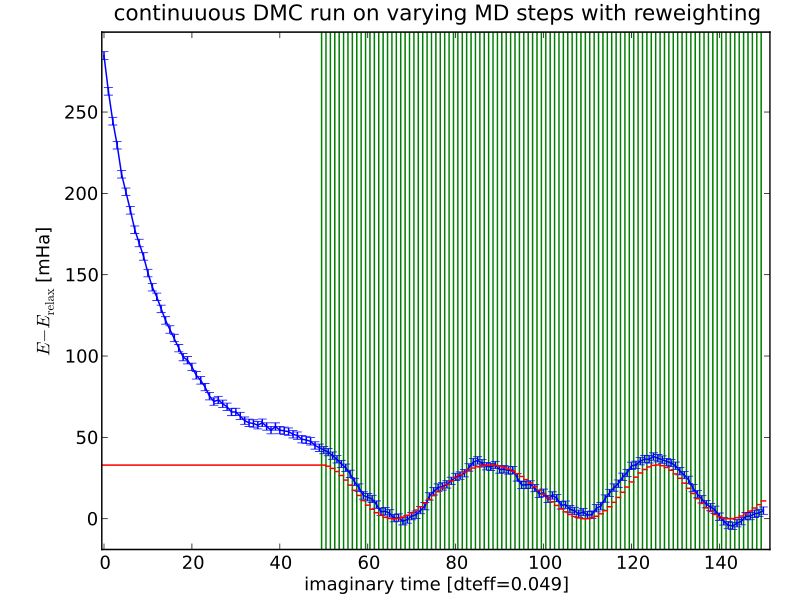
95.6 DMC MD calculation - single timestep with reweighting
Figure 4: Energies of continuous QMC-MD run
• DFT trajectory for large amplitude (1790 K)
• continuous DMC-MD run along trajectory
• no relaxation between steps
• Npop = 100000
• dtdmc = 0.05
→ Reweighting efficiency is around 99%
→ DMC energies follow the DFT energies within numerical precision.
→ fixed offset between energies given by energy difference in equilibrium position
105.7 Larger MD steps
Figure 5: Similar to previous run, except the folloing:
• pick only every 10th MD step
• compute 10 time steps for each (1 equil, 9 stats)
• population 100000
→ Reweighting efficiency: 60 ... 99 %
→ No re-equilibration necessary
115.8 Use space warping
Figure 6: Identical to previous run, except:
• space warping activated
→ Reweighting efficiency: unchanged at 60 ... 99 %
Results are near identical. Even the reweighting efficiencies are similar for each transition.
only reweighting with space warping
1→11 88.51 % 87.90 %
11→21 65.43 % 64.16 %
21→31 79.24 % 78.32 %
31→41 97.98 % 97.91 %
41→51 94.63 %
51→61 69.69 %
61→71 69.67 %
71→81 99.07 %
81→91 79.86 %
Table 1: Comparison of reweighting efficiencies for individual MD step transitions.
Open Issue: It is not quite clear why space warping would be very effective for the step in Sec. 5.4
12but have no signficant effect at all in this case.
5.9 Without reweighting
Perhaps we should have performed this test earlier...
Figure 7: Same as before but without any reweighting or space warping → no clear difference to
the results before!
5.10 Conclusions of these initial studies
The main conclusions from these tests are as follows:
• Continuous DMC is a very efficient way to eliminate equilibration times
• Reweighting does not seem to be necessary at all for this system. The bulk of the DMC
equilibration does not seem to be sensitive to the exact configuration. A population that is
equilibrated on one wave function is already mostly equilibrated for any similar wave function.
This may be true for very homogeneous crystalline systems in general.
• The only expected benefit of space warping is the improvement of the reweighting efficiency.
For this system, this improvement was not observed. Though this could be due to the fact
that electrons are not tightly bound to specific nuclei but rather distributed over the whole
crystal, it is not clear why space warping would be very effective in Sec. 5.4 but not at all in
Sec. 5.8. (→Open Issue)
• For this MD time series, the difference between DFT, VMC and DMC energy is completely
dominated by a constant offset. DMC does not show any distinct physical features that could
not be observed with less expensive methods. Though it is demonstrated that reweighting
13and space warping are effective in this case, it is not clear yet how it will perform for systems
where the use of DMC is actually of interest.
The Silicon crystal featured only a constant energy difference between the energies from DFT,
VMC and DMC. In this situation, DMC does not offer much benefit over VMC.
The really interesting question is:
What happens if the difference between VMC and DMC energy is not constant?
The real purpose of DMC is not to improve the absolute energy but to explore new physics or obtain
more accurate physically relevant energy differences. The computational cost of DMC calculations
is only justified if the DMC energy landscape is different from the VMC energy by more than just
a constant offset.
It is clear that such DMC-specific features need the DMC imaginary time evolution to develop.
A reweighting procedure that is based on the ratio of trial wave functions cannot be expected to
accurately reproduce features that are not present in the trial wave functions.
It would therefore be of great interest to study a system where the DMC energy shows distinct
features that are qualitatively different from VMC. Van der Waals complex are such systems as the
necessary correlations are present in DMC but not in VMC.
For the moment, it seems best to release the DMC-MD facility to the community and see what
they find!
6 Incorporation of the DMC-MD functionality into the CASINO
distribution
The second phase of development under MDT has been devoted to full incorporation of the DMC-
MD functionality into the public version of casino and into various supporting DFT codes. It was
desirable (1) to do this in a ‘user-friendly’ manner such that DMC-MD calculations involving a
rather complicated harnessing of two different codes could be executed by typing a simple command,
and (2) that this works out of the box on all of the many architectures that casino supports (from
single-core PCs to petascale supercomputers with batch queues).
The result is that DMC-MD is now fully integrated into the current version of casino. It appeared
for the first time in a full public release (version 2.10) in November 2011.
Following negotiations by MDT with Paolo Giannozzi and other leaders of the quantum espresso
project (which includes the pwscf DFT code), full integrated support for DMC-MD calculations
with casino has been incorporated into version 4.3 and subsequent releases of that code. The
relevant procedures are fully documented in the pwscf manual. Discussions regarding support for
other DFT codes such as castep and abinit are ongoing.
The new utilities and required changes to be described are:
1. casino support in pwscf.
2. Pseudopotentials and their converters.
143. The runpwscf script.
4. The runqmcmd script.
6.1 CASINO support in PWSCF
As has previously been noted, the interface between the two codes is provided through a file with a
standard format containing geometry, basis set, and orbital coefficients, and the official distribution
of pwscf will now compute and write out this on demand. For SCF calculations, the name of this
file may be pwfn.data, bwfn.data or bwfn.data.b1 depending on user requests (see below). If
the files are produced from an MD run, the files have a suffix .1, .2, .3 etc. corresponding to the
sequence of timesteps.
casino support is implemented by three routines in the PW directory of the quantum espresso
distribution:
• pw2casino.f90 : the main routine
• pw2casino write.f90 : writes the casino xwfn.data file in various formats
• pw2blip.f90 : does the plane-wave to blip conversion, if requested
Relevant behaviour of pwscf may be modified through an optional auxiliary input file, named
pw2casino.dat (see below).
The practical procedure for generating xwfn.data files with pwscf is as follows.
When running pwscf natively without using any of the tools provided with the casino distribution,
use the ‘-pw2casino’ option when invoking the executable pw.x, e.g.:
pw.x -pw2casino < input file > output file
The xfwn.data file will then be generated automatically.
If running using the casino-supplied runpwscf script, then one would type (with assumed in.pwscf
and out.pwscf i/o):
runpwscf --qmc OR runpwscf -w
On parallel machines, one could type e.g.
runpwscf --qmc -p 120
to run the calculation on 120 cores, or whatever..
pwscf has now been made capable of doing the plane wave to blip conversion directly (the blip
utility provided in the casino distribution is not required) and so by default, pwscf produces the
binary blip wave function file bwfn.data.b1 .
Various options may be modified by providing a file pw2casino.dat with the following format
(which follows the standard pwscf input format):
&inputpp
blip_convert=.true.
blip_binary=.true.
15blip_single_prec=.false.
blip_multiplicity=1.d0
n_points_for_test=0
/
Some or all of the five keywords may be provided, in any order. The default values are as given
above (and these are used if the pw2casino.dat file or any particular keyword is not present).
The meanings of the keywords are as follows:
blip convert
Reexpand the converged plane-wave orbitals in localized blip functions prior to writing the casino
wave function file. This is almost always done, since wave functions expanded in blips are consider-
ably more efficient in quantum Monte Carlo calculations. If blip convert=.false. a pwfn.data
file is produced (orbitals expanded in plane waves); if blip convert=.true., either a bwfn.data
file or a bwfn.data.b1 file is produced, depending on the value of blip binary (see below).
blip binary
If .true., and if blip convert is also .true, write the blip wave function as an unformatted binary
bwfn.data.b1 file. This is much smaller than the formatted bwfn.data file, but is not generally
portable across all machines.
blip single prec
If .false. the orbital coefficients in bwfn.data(.b1) are written out in double precision; if the
user runs into hardware limits blip single prec can be set to .true. in which case the coefficients
are written in single precision, reducing the memory and disk requirements at the cost of a small
amount of accuracy.
blip multiplicity
The quality of the blip expansion (i.e., the fineness of the blip grid) can be improved by increasing
the grid multiplicity parameter given by this keyword. Increasing the grid multiplicity results in
a greater number of blip coefficients and therefore larger memory requirements and file size, but
the CPU time should be unchanged. For very accurate work, one may want to experiment with
grid multiplicity larger that 1.0. Note, however, that it might be more efficient to keep the grid
multiplicity to 1.0 and increase the plane wave cutoff instead.
n points for test
If this is set to a positive integer greater than zero, pwscf will sample the wave function, the
Laplacian and the gradient at a large number of random points in the simulation cell and compute
the overlap of the blip orbitals with the original plane-wave orbitals:
hBW |P W i
α= p
hBW |BW ihP W |P W i
The closer α is to 1, the better the blip representation. By increasing blip multiplicity, or by
increasing the plane-wave cutoff, one ought to be able to make α as close to 1 as desired. The
number of random points used is given by n points for test.
166.2 Pseudopotentials and their converters
DFT trial wave functions must clearly be generated using the same pseudopotential as in the
subsequent QMC calculation. This requires the use of tools to switch between the different file
formats used by the two codes. As part of this project, we have reviewed and updated the available
tools and made sure that the utilities supplied with the official pwscf distribution meet modern
standards.
casino uses the ‘casino tabulated format’; the new version of pwscf officially supports the UPF
version 2 (UPFv2) format (though it will read other now-deprecated formats). It should be noted
that commonly-used ultrasoft and PAW pseudopotentials cannot be used with the casino code
(and previously missing error traps that block users from attempting to do so have now been
implemented).
The final status of these utilities is as follows:
casino2upf/upf2casino
These tools convert casino tabulated format to and from UPF version 2 (UPFv2) format; they
are now included in the Quantum Espresso distribution (see directory upftools). Before now the
pwscf/casino pseudopotential conversion tools used deprecated formats. The conversion to the
UPFv2 was assisted by Simon Binnie.
In the casino distribution, the directory utils/pseudo converters/pwscf/casino2upf contains
the relevant documentation.
casino2gon
Converts casino tabulated format to the (deprecated) GON format.
This is included in the utils/pseudo converters/pwscf/casino2gon directory in the casino
distribution.
Which utility to use? Since UPFv2 is now the current official format for pwscf, one would normally
use the casino2upf converter (though as of 2011 pwscf retains the ability to read GON files).
The casino2gon alternative is useful when interpolation is required - e.g. due to the use of a
non-standard grid or wave functions on a different grid. In particular it can take pp gaussian or
pp gamess as input as well as the standard pp.data - see the casino pseudopotential website at:
http://www.tcm.phy.cam.ac.uk/∼mdt26/casino2 pseudopotentials.html
6.3 The runpwscf script
The casino distribution has a sophisticated system for incorporating system-specific parameters
into the procedures for compiling and running the code. The intention is that the code will compile
out of the box by typing ‘make’, and that the code will run automatically on any known ma-
chine - including ‘difficult’ machines with customized batch queue systems - by typing ‘runqmc’
(potentially with some command-line arguments to indicate e.g. the required number of proces-
sors). This is done through the definition of a single environment variable ‘CASINO ARCH’. ‘Generic’
CASINO ARCHs are intended to represent classes of systems (such as single- or multi-processor work-
stations with particular compilers, or clusters/supercomputers with particular compilers and queue-
ing systems). However, one may also define ‘extended’ CASINO ARCHs intended to represent specific
systems which may have been customized. All these CASINO ARCHs are defined by individual files in
17the CASINO/arch/data directory (usually these may be generated automatically using the supplied
arch info utility).
As a DMC-MD calculation involves running both codes it is desirable to make pwscf understand
the CASINO ARCH system, so that it may be run automatically in the same way as casino on
any known architecture. To this end I have written a ‘runpwscf’ script which behaves in essentially
the same way as runqmc. Like runqmc, runpwscf also does extensive error checking on the given
input (including pseudopotential files) so that errors are spotted immediately rather than after
many hours of sitting in a batch queue.
The script is invoked as follows:
runpwscf [] [[--] ]
The script will run the pwscf calculations set up in where is ‘.’
by default. can be given as GNU-style long options (‘--option[=value]’) or as UNIX-
style short options (‘-abc -de -f...’, where the space between ‘-x’ and
‘’ is optional).
The most important option for our purposes is ‘--qmc’ (or equivalently -w) which flags the creation
of a casino wave function file. The full list of options is given below:
Options available on all machines
--force | -f
Run the calculation without checking for presence/correctness of input
files.
--check-only | -c
Stop before running the calculation. In clusters, this option can be used
to produce the batch submission script for manual checking; ’--check-only
--force’ would only produce a submission script in these systems.
--version= | --opt | --dev | --debug|-d | --prof
Select the binary version , which ought to be one of ’opt’, ’dev’,
’debug’ or ’prof’. --opt, --dev, --debug and --prof are equivalent to
the respective --version= option. -d sets to ’debug’.
is set to ’opt’ by default.
--chome= | -H
Set the location of the CASINO installation to . By default,
is set to \$HOME/CASINO.
--ehome= | -E
Set the location of the Espresso installation to . By default, this
is set to \$HOME/espresso.
--binary= | -b
Set the binary name to use to instead of ’pw.x’. This only needs
to be used for custom compilations with the option ’EXECUTABLE=’.
18--tpp= | -t
Set the number of OpenMP threads per process to . This requires having
compiled the code with OpenMP support, as in ’make Openmp’
--qmc | -w
Generate a CASINO wave function file (equivalent to running PWSCF with
the -pw2casino option). Output may be pwfn.data, bwfn.data or binary
bwfn.data.b1 file, depending on flags set in optional pw2casino.dat file
(see CASINO/PWSCF documentation).
--help | -h
Display this help. If the CASINO_ARCH can be determined and exists, the
help will display options specific to the current manchine, else all options
will be displayed.
--verbosity= | -v | -q
Set the verbosity level of the machine set-up process to . By
default is 0. ’-v’ increases the verbosity level by 1, and
’-q’ decreases it by 1.
Options available on workstations
--background | -B
Run PWSCF in the background, returning control to the shell after starting
the run. This has the same effect as ’runpwscf & disown’, whereby the
PWSCF process is detached from the shell, so if one wants to stop the run
’kill’ or ’killall’ must be used. It is safe to log out after running with
this option, the calculation will continue - no need for nohup/disown.
Running multiple jobs causes them to run in the background whether this
option is specified or not.
--print-out | -P
Print out the output of PWSCF as it is being run. Implies --background.
[CTRL]-[C] will stop the print-out, and the PWSCF job will remain in the
background. This option is ignored when running multiple jobs.
--gdb | -g
Run the code through the gdb debugger. This automatically sets to
’debug’ if no version had been selected. The gdb debugger works better with
some compilers than others; GCC’s gfortran is the obvious choice for using
gdb.
Options available on parallel workstations and clusters
--no-mpi | -1
Run the binary directly without invoking mpirun etc. This option is applied
before any others, and makes this script behave as if the machine was a
19single-core machine.
--nproc= | -p
Set the number of MPI processes to . This will have to be consistent
with , , and the machine information in the relevant
.arch file.
--ppn=
Set the number of MPI processes per physical, multi-core node to .
This will have to be consistent with , , , and the
machine information in the relevant .arch file.
--shmem[=] | -s
Enable shared memory.
If is provided, set the number of processses among which to share
memory to . This option requires having compiled the code with
shared memory support.
--diagram | -D
Draw a diagram of the processes and threads on each node to the terminal
during set-up.
Options available on clusters
--no-cluster | -l
Run the calculation directly on the login node of a cluster without
producing a submission script. This option is applied before any others,
and makes this script behave as if the machine was a multi-core workstation.
--nnode= | -n
Set the number of physical, (possibly) multi-core nodes to use to .
This will have to be consistent with , , and the machine
information in the relevant .arch file.
--walltime= | -T
Set the wall-time limit for the run to , given in the format
[d][h][m][s].
--coretime= | -C
Set the core-time (i.e., wall-time times number of reserved cores) limit for
the run to , given in the format
[d][h][m][s].
--name= | -N
Set the submission script name and job name to .
206.4 The runqmcmd script
The runqmcmd script is used to automate DMC-MD molecular dynamics calculations using casino
and the pwscf DFT code (which must be version 4.3 or later). Usage is :
runqmcmd [--help --nproc_dft=I --splitqmc[=N] --startqmc=M
--dft_only/--qmc_only []
We first generate a full DFT trajectory. We then do a full QMC calculation for the initial nuclear
configuration of the trajectory, followed by a series of very quick (a few moves) DMC calculations
for each point along the trajectory, where each such calculation is restarted from the config.out
of the previous one with slightly different nuclear coordinates.
This script works by repeatedly calling the runpwscf and runqmc scripts which know how to run
pwscf/casino on any individual machine. Almost all optional arguments to this script are the
same as for runpwscf/runqmc and are passed on automatically to these subsidiary run scripts (the
–background/-B option is also used by runqmcmd, and for the same purpose). Type ‘runpwscf
--help’ or ‘runqmc --help’ to find out what these options are (or see the previous section of the
manual). There is a short list of optional flags specific to runqmcmd which are described below.
It is assumed that pwscf lives in $HOME/espresso and casino lives in $HOME/CASINO. There are
override options available if this is not the case.
If you are running on a multi-user machine with an account to be charged for the calculations, you
might consider aliasing runqmcmd using e.g. alias runqmcmd="runqmcmd --user.ACCOUNT=CPH005mdt
" or whatever.
In general you should do something like the following:
Setup the pwscf input (‘in.pwscf’) and the casino input (‘input’ etc. but no wave function file)
in the same directory. For the moment we assume you have an optimized Jastrow from somewhere.
Have the sc pwscf setup as ‘calculation = "md"’, and ‘nstep = 100’ or whatever. The runqmcmd
script will then run pwscf once to generate 100 xwfn.data files, then it will run casino on each
of the xwfn.data. The first will be a proper DMC run with full equilibration (using the values of
dmc equil nstep, dmc stats nstep etc. The second and subsequent steps (with slightly different
nuclear positions) will be restarts from the previous converged config.in - each run will use new
keywords dmcmd equil nstep and dmcmd stats nstep (with the number of blocks assumed to
be 1. The latter values are used if new keyword dmc md is set to T, and they should be very
small).
It is recommended that you set dmc spacewarping and dmc reweight conf to T in casino
input when doing such calculations.
The calculation can be run through pwfn.data, bwfn.data or bwfn.data.bin (and obsolete
bwfn.data.b1) formats as specified in the pw2casino.dat file (see elsewhere).
Default behaviour of runqmcmd (on all machines)
Note : in what follows, nmdstep is the value of the pwscf input keyword ‘nstep’, while xwfn.data
refers to whatever wave function file is specified in the pw2casino.dat file (either bwfn.data.b1/bwfn.data.bin
[default], bwfn.data or pwfn.data).
For a complete DMC-MD run, the following three steps are performed in sequence:
21(A) Generate nmdstep+1 xwfn.data.$ files, where $ is a sequence number from 0 to nmdstep.
(B) Do a full DMC run on xwfn.data.0
(C) Temporarily modify the casino input file, by changing dmc md from F to T, and runtype
from vmc dmc to dmc dmc. Run nmdstep restarted QMC runs on xwfn.data.1 to xwfn.data.[nmdstep],
each restarting from the previous.
On batch queue systems, runqmcmd will by default do two batch script submissions, the first -
handled by the runpwscf script - executing step (A), and the second - handled by the runqmc
script - executing steps (B-C).
In principle, this wastes some unnecessary time (the time spent waiting for the QMC batch script
to start) but this is unavoidable if runqmcmd uses separate runpwscf and runqmc scripts to handle
the DFT and QMC calculations. This may be changed in the future, if anyone can be arsed.
Note that all calculations will be done on the number of cores requested on the command line
(with the --nproc/-p flag) irrespective of whether they are DFT or QMC calculations. You may
override this for the DFT calcs by using the --nproc dft flag to runqmcmd.
Modifications to default behaviour (on all machines)
runqmcmd --dft_only
Execute only step(1), generating nmdstep+1 xwfn.data.$ files.
Essentially the same thing can be done by executing ‘runpwscf --qmc’ but doing that would bypass
a few error traps.
runqmcmd --qmc_only
Execute only steps(B-C). This requires that the nmdstep+1 xwfn.data.$ files already exist - if
they don’t the script will whinge and die.
runqmcmd --startqmc=M
Start the chain of QMC runs with file xwfn.data.M If M = 0, the first run will be a full QMC run
with dmc md=F, otherwise if M > 0 then all runs will be short restarted ones with dmc md=T.
(Note that for M > 0, dmc md and runtype in the input file will be temporarily ‘modified’ as
described above, no matter what values they currently have).
Modifications to default behaviour (batch machines only)
On batch machines, there is an additional complication due to the walltime limits on particular
queues which may require full DMC-MD runs to be split into sections. The following flags may be
used to do this.
runqmcmd --splitqmc
Do step A (DFT run), step B (initial QMC run) and step C (chain of remaining QMC restarted
jobs) as three separate batch script submissions (i.e. no longer combine B and C).
22runqmcmd --splitqmc=N
As (3) but split step C into N separate batch script submissions.
Example : nmdstep=1005, and runqmcmd --splitqmc=4 will result in 1 step B job plus four sets
of step C jobs with 251, 251, 251, 252 steps.
Note finally that there are a couple of simple utilities (extr casino and extr pwscf that extract
the DFT/QMC energies from the output of a runqmcmd run.
7 Other work
The previous sections have detailed the work to implement DMC-DFT molecular dynamics in
casino, which was the main aim of the current project. As this was completed well within the
allotted timeframe, I (MDT) have used the remainder of the time to work on some other short
projects related to casino development. The most important of these was a project to improve
the parallel efficiency of casino on massively parallel computers, potentially allowing the code to
be run on hundreds of thousands or even millions of cores with quasi-perfect parallel efficiency.
Following a description of this work, I go on to list my other more minor improvements to the
CASINO distribution.
7.1 Full parallel efficiency on parallel computers
7.1.1 Introduction
Quantum Monte Carlo is in general an intrinsically parallel technique, and as such is ideally placed
to exploit new and future generations of massively parallel computers. This is trivially realized in
the case of variational Monte Carlo (VMC) and in the various associated techniques for carrying
out VMC wave function optimization. In the pure VMC case, essentially no interprocessor commu-
nication is required during a simulation. Each processor carries out an independent random walk
using a fixed wave function and a different random number sequence. The resulting energies are
then averaged over the processors at the end. Assuming the equilibration time to be negligible,
running for a length of time T on Np processors generates the same amount of data as running
for time Np T on a single processor (though of course the results will only agree within statistical
error bars since the random walks are different in the two cases). VMC should therefore scale to
an arbitrarily large number of processors (as, for reasons we shall not go into, do the various wave
function optimization algorithms).
The problem - if there is a problem - therefore lies in the DMC algorithm, and this is largely to do
with load balancing. DMC is parallelized in a similar way to VMC - by assigning separate walkers
to different processors - but in DMC by contrast the processors are required to communicate. The
branching algorithm that it uses leads to a dynamically variable population of walkers, that is, the
population fluctuates during the run as walkers are killed or duplicated to ‘change the shape of
the wave function’. One of the reasons that this leads to interprocessor communication is that the
population must be adjusted dynamically to some initial target via a kind of feedback mechanism as
the simulation proceeds. This relies on a knowledge of the instantaneous total energy, which must
be calculated and averaged over all processors after each time step. The most important problem,
however, is the necessity to transfer walkers between the cores (a walker, in this sense, being the list
23of current electron positions for the configuration, along with various associated quantities related
to the energy and wave function). These transfers are purely for efficiency; in order to maintain
load balance it is important to ensure that each core has roughly the same number of walkers, since
the cost of each time step is determined by the processor with the largest population. The total
number of walkers communicated between processors increases with the number of cores and ends
up being the single greatest cause of inefficiency for runs on massively parallel machines. A rough
theoretical analysis of the expected scaling behaviour might run as follows.
The time tmove required to propagate each walker scales as Neα , where Ne is the number of particles,
and α is an integer power. For typical systems, where extended orbitals represented in a localized
basis are used and the CPU time is dominated by the evaluation of the orbitals, α = 2. The use
of localized orbitals can improve this to α = 1. For very large systems, or systems in which the
orbitals are trivial to evaluate, the cost of updating the determinants will start to dominate: this
gives α = 3 with extended orbitals and α = 2 with localized orbitals. Hence the average cost of
propagating all the walkers over one time step, which is approximately the same on each processor,
is
N α Ntarget
TCPU ≈ a e , (1)
Nproc
where a is a constant which depends on both the system being studied and the details of the
hardware, Ntarget is the target population, and Nproc is the number of processors.
So now the population varies on each processor. How? Let nredist τ be the redistribution period, that
is, we redistribute the walker population after every nredist time steps τ . Given the exponential form
of the branching factor, the population on a processor p at any given time must be increasing or de-
creasing exponentially, because the mean energy E(p) of the walker population on that processor is
unlikely to be exactly equal to the reference energy ET in the argument of the branching factor. We
assume that E(p) − ET remains roughly constant over the redistribution period. At the start of the
redistribution period the population Nw (p, 0) on each processor is the same. At the end of the redis-
tribution period, the expected population on processor p is Nw (p, nredist ) = Nw (p, 0) exp[−(E(p) −
ET )nredist τ ]. Hence N̄w (nredist ) ≈ N̄w (0) exp[−(Ē − ET )nredist τ ] + O(n2redist τ 2 ), where the bar de-
notes an average over the processors, and so the average growth or decay of the population is the
same as that of the entire population (which should be small, because ET is chosen so as to ensure
this).
What is the optimal redistribution period? Recall tmove is the cost of propagating a single walker
over one time step. Let ttrans be the cost of transferring a single walker between processors. Let q
be the processor with the largest number of walkers, i.e., the one with the lowest energy E(q) ≡
min{E(p)}. Both the cost of propagating walkers and the cost of transferring them are determined
by processor q. The expected number of walkers on processor q at the end of the redistribution
period (i.e., after nredist time steps) is max{Nw (p, nredist )} ≈ N̄w (nredist )+cnredist +O(n2redist ), where
c = N̄w (1)(Ē − min{E(p)})τ . Here hN̄w (0)i = Ntarget /Nproc and hci is a positive constant. At the
end of the redistribution period, cnredist walkers are to be transferred from processor q. Hence the
average cost of transferring walkers per time step is ttrans hci, which is independent of nredist .
The average cost per time step of waiting for the processor q with the greatest number of walkers
to finish propagating all its excess walkers is
tmove hci [0 + 1 + . . . + (nredist − 1)] tmove hci(nredist − 1)
= . (2)
nredist 2
24So the total average cost per time step in DMC is
tmove Ntarget tmove hci(nredist − 1)
T = + + ttrans hci. (3)
Nproc 2
Clearly the redistribution period should be chosen to be as small as possible to minimize T . Nu-
merical tests confirm that increasing the redistribution period only acts to slow down calculations.
One should therefore choose nredist = 1, i.e., redistribution should take place after every time step.
We assume this to be the case henceforth.
What, then, is the cost of load balancing? Let σE(p) be the standard deviation of the set of
p
processor energies. We assume that hE(p)i − hmin{E(p)}i ∝ σE(p) ∝ Ne Nproc /Ntarget . Hence
p
hci ∝ Ne Ntarget /Nproc . The cost ttrans of transferring a single walker is proportional to the system
size Ne . Hence the cost of load balancing is
s
Ntarget Ne3
Tcomm ≈ b , (4)
Nproc
where the constant b depends on the system being studied, the wave-function quality and the com-
puter architecture. Note that good trial wave functions will lead to smaller population fluctuations
and therefore less time spent load-balancing.
Clearly one would like to have TCPU
Tcomm , as the DMC algorithm would in theory be perfectly
parallel in this limit. The ratio of the cost of load balancing to the cost of propagating the walkers
is
Tcomm b Nproc 1/2 3/2−α
= Ne . (5)
TCPU a Ntarget
It is immediately clear that by increasing the number of walkers per processor Ntarget /Nproc the
fraction of time spent on interprocessor communication can be made arbitrarily small. In practice
the number of walkers per processor is limited by the available memory, and by the fact that carrying
out DMC equilibration takes longer if more walkers are used. Increasing the number of walkers does
not affect the efficiency of DMC statistics accumulation, so, assuming that equilibration remains a
small fraction of the total CPU time, the walker population should be made as large as memory
constraints will allow.
For α > 3/2 (which is always the case except in the regime where the cost of evaluating localized
orbitals dominates), the fraction of time spent on interprocessor communication falls off with system
size. Hence processor-scaling tests on small systems may significantly underestimate the maximum
usable number of processors for larger problems.
So that’s the theory; how does this work in practice? In analyzing scaling behaviour one normally
distinguishes between ‘strong scaling’ - where we ask how the time to solution for a fixed system size
varies with the number of processors - and ‘weak scaling’ where we ask how the time to a solution
varies for a fixed system size per processor (i.e. if we double the number of processors, we double
the size of the system). Perfect weak scaling is thus a constant time to solution, independent of
processor count.
What is the appropriate definition of ‘system size’ in this context? One would think that QMC is
different from DFT, of course, since if we double what we normally consider to be the size of the
system (the number of electrons in the molecule, or whatever) then we must double the number of
samples of the wave function in order to get the same error bar. So our criterion for the system
25size, is something like ‘the number of samples of the wave function configuration space required to
get a fixed error bar’. In all the scaling calculations reported here, we report the time taken to
sample the wave function N times, where N is the number of walkers times the number of moves.
N is constant for all core counts, therefore we are looking at the strong scaling.
Two ways of doing this have been considered. The first way is to consider both a fixed total target
population of walkers and a fixed number of moves, neither of which varies with the number of
processors. For a code that scaled ideally one would then expect the time taken to halve if we double
the number of processors since each individual processor will have half the number of walkers to
deal with. This is usually not the best way to exploit QMC on a parallel machine, but it serves to
illustrate several important points.
[CPU time (1296 cores) / CPU time (N cores) ] * 1296
80000 Ideal linear scaling
CASINO 2.6
Modified CASINO
60000 FIXED TARGET POPULATION
40000
20000
0
0 20000 40000 60000 80000
Number N of processor cores (JaguarPF)
Figure 8: Scaled CPU time required by various numbers of cores of the JaguarPF machine to
carry out one ten-move DMC statistics accumulation block for a water molecule adsorbed on a
two-dimensionally periodic graphene sheet containing fifty carbon atoms per cell, using both the
September 2010 version of casino 2.6 (solid-red line) and my newly modified version of casino
(dotted blue line). For comparative purposes ‘ideal linear scaling’ is shown by the solid black line.
Fixed target of 486000 for total walker population. Note that fixing the total target population can
introduce considerable inefficiency at higher core counts and this graph should not be looked on as
representing the general scaling behaviour of the casino program. This inefficiency can generally
be decreased by increasing the number of walkers per core.
In Fig. 8 we display timing data of this nature obtained with casino in a typical DMC simulation
for a system of one water molecule adsorbed on a graphene sheet represented by a 2D periodic cell
containing fifty carbon atoms. The initial number of walkers and the subsequent target population
26is fixed at 486000. The graph shows the parallel performance of casino on the JaguarPF machine
(a Cray XT5 machine with 224256 cores, at Oak Ridge National Laboratory, U.S.A. which - at
the time of this work in Jan 2011 - was listed in second position on the Top 500 supercomputer
list). Because of the nature of the multi-core processors on this machine the core count must be a
multiple of twelve. We therefore start with 684 cores, and progressively double it seven times. The
CPU time taken on 648, 1296, 2592, 5184, 10368, 20736, 41472 and 82944 cores to do one block
of ten DMC statistics accumulation moves for 486000 configurations was, respectively, 5787, 2867,
1452, 742, 389, 230, 159, 216 seconds. In plotting the data we have rescaled it (by dividing by the
time taken for the 1296-core case and multiplying by 1296) in order to display the deviation from
linear scaling. Focussing on the red solid line for CASINO 2.6 in the diagram, one can see that
that pretty good scaling is obtained up to around 20000 cores, but beyond that the performance
starts to fall away, and the code is actually slower the more processors are used beyond around
50000 cores.
Is it possible to improve this behaviour? I have investigated this problem, and it turns out to
be possible to substantially improve the performance, and even to effectively eliminate the cost
of walker redistribution completely. The improved performance was obtained via the following
strategies:
(1) The use of asynchronous, non-blocking communications. CASINO uses the standard Message
Passing Interface (MPI) to handle interprocessor communication. Using this software to send a
message from one processor to another, one might typically call blocking MPI SEND and MPI RECV
routines on a pair of communicating processors. All other work will halt until the transfer com-
pletes. However, one may also use non-blocking MPI calls, which allow processors to continue doing
computations while communication with another processor is still pending. Another advantage is
that if used correctly, some internal MPI buffers may be bypassed with a dramatic increase in
the communication bandwidth. On calling the non-blocking MPI ISEND routine, for example, the
function will return immediately, usually before the data has finished being sent.
Bearing this in mind, the casino DMC algorithm has now been modified to do something like the
following:
MOVE 1
- Move all currently existing walkers forward by one time step
- Compute the multiplicities for each walker (the number of copies of each
walker to continue in the next move).
- Looking at the current populations of walkers on each processor, and at the
current multiplicities, decide which walkers to send between which pairs of
processors, and how many copies of each are to be created when they reach
their destination.
- Sending processors initiate the sends using non-blocking MPI_ISENDs; receiving
processors initiate the receives using non-blocking MPI_IRECVs. All continue
without waiting for the operations to complete.
- Perform on-site branching (kill or duplicate walkers which require it on any
given processor).
27MOVE 2 AND SUBSEQUENT MOVES
- Move all currently existing walkers on a given processor by one time step (not
including walkers which may have been sent to this processor at the end of the
previous move).
- Check that the non-blocking sends and receives have completed (they will
almost certainly have done so) using MPI_WAITALL. When they have, duplicate
newly-arrived walkers according to their multiplicities and move by one time
step.
- Compute the multiplicities for each moved walker.
- Continue as before
It was also found necessary to:
(2) Parallelize the procedure for deciding which walkers to send between which pairs of processors,
as follows.
Having received a report of the current population of walkers on each core, the master computes
a set of instructions for the walker transfers. The algorithm aims to produce the fewest possible
number of transfers by carefully matching the requirements of receiving processors (those with a
population less than the target) and the availability and multiplicity of surplus walkers on sending
processors (those with a population greater than the target). For example, if processor A had a
deficit of five walkers and processor B had a surplus of one walker with a multiplicity of four, then
both target populations could be satisfied by the transfer of one walker (which would duplicate
itself four times on arriving at the destination processor). This is quite clearly more efficient than
having five separate processors transfer one walker each to processor A, or by processor C sending
five separate walkers each with a multiplicity of one to processor A.
Unfortunately doing this process carefully and exactly (working out on the master a set of optimally-
efficient instructions for each processor, and sending the instructions from the master to the slaves)
scales linearly with the number of processors, and eventually the cost of working out the most
efficient transfers becomes more expensive than doing the transfers themselves. This is the sort of
thing that is easily missed in formal analyses, but for very large numbers of processors this was
the rate limiting step in casino. It is quite easy to fix, for example, by only considering transfers
in small ‘redistribution groups’ of around 500 cores which are large enough for a full set of ‘good
matches’ to be made (though it is important that the cores associated with each group are ‘shuffled’
after every move to prevent inequalities of population developing between groups). Having done
this for our test case the time taken to create and broadcast the whole set of transfer instructions
for the ten-move block was only a second or two, independent of the number of processors, rather
than a few hundred seconds as was the case on 82944 processors of the JaguarPF machine.
Taken together, these improvements (together with some other more minor refinements) have ef-
fectively removed the cost of redistributing and branching in casino, as shown by the timings in
Table 2. For the largest number of cores studied, the new redistribution algorithm was over 270
times faster. The improvements to the scaled timing data are also shown in Fig. 8 as the dashed
28blue line (in terms of raw data, the CPU time required for a ten move block of DMC statistics ac-
cumulation moves on 648, 1296, 2592, 5184, 10368, 20736, 41472 and 82944 cores was, respectively,
5767, 2883, 1462, 743, 382, 221, 115, and 68 seconds).
Number of cores Time, casino 2.6 (s.) Time, Modified casino (s.)
648 1.00 1.05
1296 3.61 1.27
2592 7.02 1.52
5184 18.80 3.06
10368 37.19 3.79
20736 75.32 1.32
41472 138.96 3.62
82944 283.77 1.04
Table 2: CPU time taken to carry out operations associated with redistribution of walkers between
processors in the original version of casino and in the newly-modified version, during one ten-move
DMC block for a water molecule adsorbed on a 2d graphene sheet (these numbers include ten moves
of DMC equilibration, and should be roughly halved to compare with the times quoted in the text).
So while this represents a great improvement for large core counts (the total CPU time required
for the calculation on 82944 cores was over three times faster than before) the scaling is still not
linear with the number of processors. Why? We shall use an alternative way of doing the scaling
calculations to illustrate. Previously we used a fixed target number of walkers and a fixed number
of DMC moves for all the calculations. Every time the core count was doubled, the number of
configs per processor was halved, and by 82944 cores there are only five or so walkers per processor
(down from 750 per processor in the 684-core case). Each processor was able to move these five
walkers so quickly that the time taken for various minor tasks normally considered unimportant
became significant in determining the scaling. The rate limiting step in the 82944-core case turned
out to be the summing of the energies and associated quantities over all the processors using an
MPI REDUCE operation, in preparation for computing averages over the nodes, an operation which
is difficult to make any more efficient than it already is. Interestingly, the cost of walker transfers
using the new algorithm was negligible by comparison.
It is vital therefore to ensure that each processor has enough to do during each move of the entire
ensemble of configurations, and a much better way of utilizing a massively parallel machine (if it
turns out to be possible) is to consider a large-enough fixed target number of walkers per processor,
rather than a fixed total target population. If we start with N walkers we can, at least in principle,
decrease the error bar on the answer by the same amount either by doubling the number of walkers
to 2N or by moving the N walkers for twice as many moves. Only in the latter case do we double
the amount of interprocessor communication required. We have therefore redone the calculations
using a fixed target of 100 walkers per processor. Every time we double the processor count the
total number of walkers doubles and, in order that we maintain the ‘system size’ - defined earlier
as the total number of sampling configurations of the configuration space to get a fixed error bar -
we halve the number of moves (one cannot of course do this indefinitely!). In such a case doubling
the number of processors should halve the required CPU time as before. Note that all we are really
doing here is changing how many samples we do on each core between each global communication;
we are exploiting the freedom that we are allowed in choosing the number of moves and walkers
to make sure that there is enough work for the processors to do during a move. We are, in effect,
improving the ratio in Eq. 5 in the way suggested. So, the resulting graph is shown in Fig. 9, and
29You can also read