DYNAMIC AIRLINE PRICING AND SEAT AVAILABILITY - Cowles Foundation
←
→
Page content transcription
If your browser does not render page correctly, please read the page content below

DYNAMIC AIRLINE PRICING AND SEAT AVAILABILITY

                       By

                Kevin R. Williams

                  August 2017
              Updated February 2018

COWLES FOUNDATION DISCUSSION PAPER NO. 3003U

COWLES FOUNDATION FOR RESEARCH IN ECONOMICS
               YALE UNIVERSITY
                   Box 208281
         New Haven, Connecticut 06520-8281

              http://cowles.yale.edu/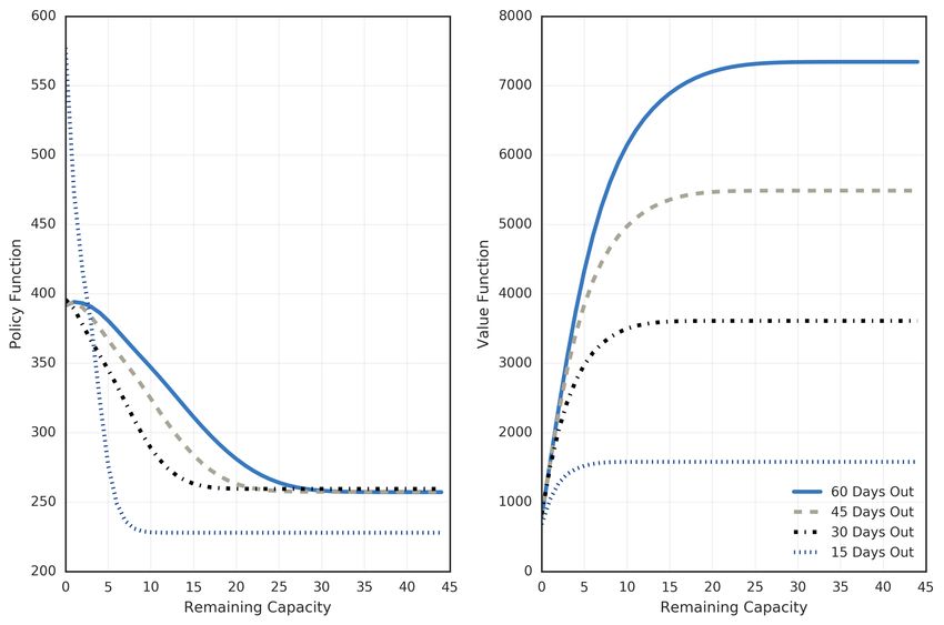
DYNAMIC AIRLINE PRICING AND SEAT AVAILABILITY

                                          Kevin R. Williams
                                       School of Management
                                            Yale University∗

                                             February 2018†

                                                  Abstract

          Airfares are determined by both intertemporal price discrimination and dynamic
       adjustment to stochastic demand. I estimate a model of dynamic airline pricing
       accounting for both forces with new flight-level data. With model estimates, I disen-
       tangle key interactions between the arrival pattern of consumer types and remaining
       capacity under stochastic demand. I show that the forces are complements in airline
       markets and lead to significantly higher revenues, as well as increased consumer sur-
       plus, compared to a more restrictive pricing regime. Finally, I show that abstracting
       from stochastic demand leads to a systematic bias in estimating demand elasticities.

       JEL: L11, L12, L93

   ∗
    kevin.williams@yale.edu
   †
    This paper is an updated chapter of my dissertation at the University of Minnesota. I thank Tom Holmes,
Jim Dana, Aniko Öry, Amil Petrin, Tom Quan and Joel Waldfogel for comments. I thank the seminar
participants at the Federal Reserve Bank of Minneapolis, Yale School of Management, University of Chicago
- Booth, Georgetown University, University of British Columbia, University of Rochester - Simon, Dartmouth
University, Northwestern University - Kellogg, Federal Reserve Board, Federal Reserve Bank of Richmond,
Indiana University, Indiana University - Kelley, Marketing Science, and the Stanford Institute for Theoretical
Economics (SITE). I also thank the Minnesota Supercomputing Institute (MSI) for providing computational
resources.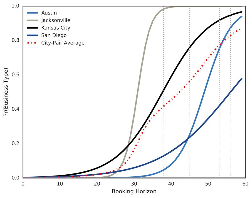
1       Introduction
          Air Asia (2013) on intertemporal price discrimination:
          Want cheap fares, book early. If you book your tickets late, chances are you are desperate to fly and
          therefore don’t mind paying a little more.1

          easyJet (2003) on dynamic adjustment to stochastic demand:
          Our booking system continually reviews bookings for all future flights and tries to predict how popular
          each flight is likely to be. If the rate at which seats are selling is higher than normal, then the price would
          go up. This way we avoid the undesirable situation of selling out popular flights months in advance.2

        Airlines tend to charge high prices to passengers who search for tickets close to their
date of travel. The conventional view is that these are business travelers and that airlines
capture their high willingness to pay through intertemporal price discrimination. Airlines
also adjust prices on a day-to-day basis, as capacity is limited and the future demand for
any given flight is uncertain. They may adjust fares upward to avoid selling out flights
in advance, or fares may actually fall from one day to the next, after a sequence of low
demand realizations.
        This paper examines pricing in the airline industry, taking into account both forces:
intertemporal price discrimination (fares responding to time) and dynamic adjustment to
stochastic demand (fares responding to seats sold). Collectively, I call this dynamic airline
pricing. I use a new flight-level data set consisting of daily fares and seat availabilities
to estimate a model of dynamic airline pricing in which firms face a stochastic arrival of
consumers. The mix of consumer types – business and leisure travelers – is allowed to
change over time, and in the estimated model, late-arriving consumers are significantly
more price-inelastic than early-arriving consumers. I use the model to quantify the welfare
effects of dynamic airline pricing, but also to establish important interactions between in-
tertemporal price discrimination and dynamic adjustment to stochastic demand in airline
    1
   Accessed through AirAsia.com’s Investor Relations page entitled, “What is low cost?"
    2
   Appeared on easyjet.com’s FAQs. Accessed through “Low-Cost Carriers and Low Fares" and “Online
Marketing: A Customer-Led Approach."

                                                                1
markets. Finally, I show that analyzing both forces together is critical to quantifying the
welfare implications of airline pricing.
The existing research documents the importance of intertemporal price discrimination
and dynamic adjustment to stochastic demand separately in airline markets, and the
central contribution of this paper is to study them jointly and quantify their interactions.
Consistent with the idea of market segmentation, Puller, Sengupta, and Wiggins (2015)
find that ticket characteristics, such as advance purchase discount (APD) requirements,
explain much of the dispersion in fares. Lazarev (2013) quantifies the welfare effects
of airline pricing by estimating a model of intertemporal price discrimination but not
dynamic adjustment. He finds a substantial role for this force.3 Escobari (2012) and
Alderighi, Nicolini, and Piga (2015) find evidence that airlines face stochastic demand and
that prices respond to remaining capacity. These results support the theoretical predictions
of Gallego and Van Ryzin (1994) and a large branch of research in operations management
that studies optimal pricing under uncertain demand, limited capacity, and limited time
to sell.4 Indeed, this research has been used to inform airline pricing algorithms.
The estimated structural model allows me establish two key points about the interac-
tion between the pricing forces. First, dynamic adjustment complements intertemporal
price discrimination in the airline industry. This is due to the fact that price-inelastic con-
sumers (i.e., business travelers) tend to buy tickets close to the departure date. To be able to
price discriminate towards these late-arriving consumers, airlines must successfully save
seats until close to their departure date. These consumers are then charged high prices.
I show that dynamic pricing more efficiently allocates capacity and increases consumer
welfare in the monopoly markets I study relative to either uniform pricing or a pricing
3
Intertemporal price discrimination can be found in many markets, including video games (Nair 2007),
Broadway theater (Leslie 2004), and concerts (Courty and Pagliero 2012). Lambrecht et. al. (2012) provide an
overview of empirical work on price discrimination more broadly.
4
An overview of the dynamic pricing literature can be found in Elmaghraby and Keskinocak (2003) and
Talluri and Van Ryzin (2005). Sweeting (2012) analyzes ticket resale markets. Pashigian and Bowen (1991) and
Soysal and Krishnamurthi (2012) study clearance sales and seasonal goods, respectively. Zhao and Zheng
(2000), Su (2007), and Dilme and Li (2016) discuss extensions to dynamic pricing models, including consumer
dynamics. Seat inventory control has also been studied; see Dana (1999).
2system in which fares vary with only the purchase time but not with past demand shocks.
Second, I show that in order to quantify the welfare effects of price discrimination in airline
markets, it is necessary to take stochastic demand into account. When abstracting from
stochastic demand, the opportunity cost of selling a seat is the same regardless of the date
of purchase. In reality, the opportunity costs tend to increase in airline markets because
of the late arrival of price insensitive consumers. As a consequence, I show an empir-
ical procedure abstracting from this feature of the market will systematically overstate
consumers’ price insensitivity. The bias is large close to the departure date.
In order to investigate dynamic airline pricing, a detailed data set of ticket purchases is
required. However, the standard airline data sets used in economic studies (e.g., Goolsbee
and Syverson (2008); Gerardi and Shapiro (2009); Berry and Jia (2010)) are either at the
monthly or the quarterly level. Recent papers use new data to get to the flight level.
McAfee and Te Velde (2006) and Lazarev (2013) create data sets containing high-frequency
fares. Other papers have obtained high frequency fares as well as a measure of seats
sold. Puller, Sengupta, and Wiggins (2015) capture a fraction of sales through a single
computer reservation system used by airlines. Escobari (2012) and Clark and Vincent
(2012) collect fare and flight availability data, with the available number of seats derived
from publicly available seat maps. I use a new data source that allows me to capture
the same information that travel agents see, such as which seats are blocked, occupied,
and available. I merge these data with daily fares and flight availability data. In total, I
track over 1,300 flights in US monopoly markets over a six-month period. I use the data
to provide descriptive evidence of both intertemporal price discrimination and dynamic
adjustment to stochastic demand.
While empirical evidence is informative, it cannot be used to disentangle the interac-
tions between the pricing forces. I proceed by estimating a structural model that contains
three key ingredients: (i) a monopolist has fixed capacity and finite time to sell; (ii) the
firm faces a stochastic arrival of consumers; and (iii) the mix of consumers, correspond-
3ing to business and leisure travelers, is allowed to change over time.5 The firm solves a
stochastic dynamic programming problem, offering a fare to consumers each day before
departure. For the demand system, I assume that a stochastic process brings consumers
to the market. The consumers that arrive know when they want to travel and solve a
static discrete choice problem.6 The demand model differs from earlier theoretical work,
including Gale and Holmes (1993), and from empirical work such as Lazarev (2013), in
which consumers are uncertain, and waiting provides more information. In my model the
only reason to wait is to bet on price, and since prices tend to increase, I show that only
a small transaction cost is needed to persuade consumers to decide whether to travel in
the period they arrive. I also provide empirical evidence that suggests this is a reasonable
assumption.7 I use the firm’s pricing decision, along with the realizations of demand, to
separately identify the arrival process of consumers and the demand elasticity over time.
Using the model estimates, I conduct a series of counterfactual exercises to quantify the
welfare implications of dynamic airline pricing and to highlight how these results depend
on the arrival process of consumers. The general finding is that, while more-restrictive
pricing systems reduce the ability of firms to price discriminate, the aggregate consumer
welfare gains are limited, or even negative, due to inefficient capacity allocation. That is,
while airlines do price discriminate, which we may think only harms consumers, their
pricing also more efficiently allocates scarce seats. In fact, under uniform pricing, revenues
drop by 2%, but aggregate consumer welfare is unchanged. In this counterfactual, leisure
consumers are charged relatively higher prices, and while business consumers are charged
relatively lower prices, many flights sell out in advance. Moreover, I find total consumer
welfare is lowered when fares are allowed to respond to the date of purchase but not to the
scarcity of seats. However, the pricing forces interact differently under alternative arrival
5
McAfee and Te Velde (2006) note that stochastic demand models that do not incorporate changes in
willingness to pay over time do not match the positive trend in airfares as the departure date approaches.
6
The specification is similar to that in Talluri and Van Ryzin (2004) and Vulcano, van Ryzin, and Chaar
(2010); however, my model also allows for the mix of consumers to change across time.
7
Li, Granados, and Netessine (2014) study dynamic consumer behavior in airline markets. Depending on
the specification, they find that between 5% and 20% of consumers are dynamic.
4processes. If price-insensitive consumers were the first to arrive, for example, dynamic
adjustment no longer complements intertemporal price discrimination, and stochastic
demand pricing is used to clear excess capacity. This is consistent with fire sales that are
commonly used in retailing.
2 Data
I create an original data set of airfares and seat availabilities with data collected from two
popular online travel services. The first is a travel search engine, owned by Kayak.com,
from which I collect daily fares at the itinerary level, with itinerary defined as a routing,
airline, flight number(s), and departure date(s) combination. I obtain all one-way and
round-trip itinerary fares for stays of less than eight days. The fares recorded correspond
to the cheapest ticket available for purchase. The fare data include the fare class and fare
basis code, which provide some information regarding the restrictions of the ticket, such
as advance purchase discount requirements.8
The second web service, operated by Expertflyer.com, allows users to look up flight
availability. I collect two sources of information. First, I obtain airline seat maps for each
flight. By comparing seat maps across time, I obtain daily bookings. Second, I collect the
fare availability (sometimes called fare buckets) for each flight. This information provides
censored information regarding which fares are available to purchase. For example, Y9
indicates that the Y class fare, which is typically the most expensive coach fare available,
has at least nine tickets available for purchase.9 In total, the sample contains 1,362 flight
departures, with each flight tracked for 60 days. All flights in my data set departed
8
G21JN5 is an example. This fare basis code indicates a G fare class ticket, and a 21-day advance purchase
discount. Lazarev (2013) has a nice discussion of airline pricing and provides additional details on fare
restrictions. Like Lazarev (2013), I model only the pricing choice and not the decision to assign restrictions or
quantities for each price.
9
Regarding the example of the fare basis code G21JN5, the fare availability data might say G5. This means
five seats remain for that particular fare. Fare availabilities can change because of ticket purchases, but also
because of changes input by managers. Both of these potentially result in changes in price, which is the focus
of this paper.
5between March 2012 and September 2012.
In the following subsections, I discuss route selection (Section 2.1) and the use of seat
maps to infer bookings (Section 2.2), and I provide summary statistics and preliminary
evidence from the data (Section 2.3).
2.1 Route Selection
I select markets in which to study using the publicly available DB1B tables, which are
frequently used to study airline markets. The DB1B tables contain 10% of domestic ticket
purchases and are at the quarterly level. The data contain neither the date flown nor the
purchase date. I define a market in the DB1B as an origin, destination, quarter. I single
out markets where:
(i) there is only one carrier operating;
(ii) there is no nearby alternative airport;
(iii) at least 95% of flight traffic is not connecting to other cities;
(iv) total quarterly traffic is greater than 3,000 passengers;
(v) total quarterly traffic is less than 30,000 passengers; and
(vi) there is high nonstop traffic.
Criteria (i) and (ii) narrow the focus to monopoly markets. One potential complica-
tion with using airline seat maps to recover bookings is that it is not clear what fare to
assign to an observed change in a seat map. Since airlines offer extensive networks, the
disappearance of a single seat could be associated with one of several thousand possible
itineraries. This is an important consideration since pricing may be different across routes,
and this is especially true with regard to feeder routes versus main routes. This issue
is addressed in (iii), which essentially rules out most routes from major hubs. Criterion
(iv) corresponds to routes with a less than 75% load factor (seats occupied / capacity) of
a daily 50-seat aircraft. This criterion removes routes with irregular service. Criterion (v)
6removes most routes with several daily frequencies. I then look for routes with (vi) high
nonstop traffic. This criterion is important for establishing the relevant outside option in
the demand model. In the data, (vi) is negatively correlated with distance (ρ = −.5). Cities
with very high nonstop traffic percentages tend to be short-distance flights, and, given
such short distances, many consumers may choose to drive instead. At the same time, the
DB1B data suggest that longer flights have lower nonstop traffic percentages, suggesting
that more consumers choose a connecting flight option.
I select four city pairs, or eight directional routings, given the selection criteria above.
All directional routings either originate or end in Boston, MA. The other cities are: San
Diego, CA; Austin, TX; Kansas City, MO; and Jacksonville, FL. The selected markets have
close to 100% direct traffic, meaning that very few passengers connect to other cities.
The percent of nonstop traffic ranges between 40% and 70%. Three of the four city pairs
are operated by JetBlue and the other by Delta Air Lines.10 The selected markets are all
low-frequency, with at most two daily frequencies.
Three other features of the data are worth noting. First, JetBlue prices itineraries at the
segment level; that is, consumers wishing to purchase round-trip tickets on this carrier
purchase two one-way tickets. As a consequence, round-trip fares in these markets are
exactly equal to the sum of the corresponding one-way fares. Since fares must be attributed
to each seat map change, this feature of the data makes it easier to justify the fare involved.
Second, JetBlue does not oversell flights, while most other air carriers do.11 I will use this
feature of the data to simplify the pricing problem in the next section. Third, JetBlue does
not offer first class on the routes studied. This allows for investigating all sales and also
controls for one aspect of versioning (first class versus economy class).12
10
At the time of data collection, flights between Kansas City and Boston were operated by regional carriers
on behalf of Delta Air Lines. Since Delta Air Lines determines the fares for this market, I collectively call these
regional carriers Delta.
11
In the legal section of the JetBlue website, under Passenger Service Plan: “JetBlue does not overbook
flights. However some situations, such as flight cancellations and reaccommodation, might create a similar
situation."
12
The Delta first class cabins were typically six seats for the market studied.
72.2 Inference and Accuracy of Seat Maps
A seat map is a graphical representation of occupied and unoccupied seats for a given
flight at a select point in time before the departure date. Many airlines that have assigned
seating present seat maps to consumers during the booking process. When a consumer
books a ticket and selects a seat, the seat map changes to reflect that an unoccupied seat is
now occupied. The next consumer wishing to purchase a ticket on the flight is offered an
updated seat map and can choose one of the remaining unoccupied seats. By differencing
seat maps across time – in this case daily – inferences can be made about daily bookings.
I use a new data source that allows me to distinguish between various types of occupied
and occupied seats.
Figure 1 presents a sample seat map: occupied seats are in solid blue, while the
unshaded blocks correspond to unoccupied seats. Seats with a "P" are available, but
classified as premium. These seats are located toward the front of the aircraft or in exit
rows. Some airlines charge a premium to be seated in these rows. Finally, the seat map
indicates seats currently blocked by the airline with "X"s. Seats that are blocked are usually
not disclosed on airline websites; however, I am able to capture these data through the
web service used. Seats may be blocked due to crew rest, weight and balance, because a
seat is broken, or because the airline reserves accessible seats for handicapped passengers
until the day of departure.13 For every seat map collected, I aggregate the number of
occupied, unoccupied, and blocked seats. I compare the aggregate counts across days to
determine bookings by day prior to departure.
13
Seat blocking may be used to encourage consumers to purchase tickets or upgrade, as they give the
impression that the cabin is closer to capacity. However, the data suggest that airlines predominantly block
seats in exit rows and at the front and/or back of the cabin until closer to the departure date or when bookings
demand additional seats. 69% of the flights in the sample experience changes in the number of blocked seats,
and while I do not model the decision to block/unblock seats, I do take this information into account when
determining bookings. Knowing which seats are blocked is important because it allows me to distinguish
between consumers’ decisions and airlines’ adjustment of the supply of seats. For example, if an airline
unblocks six seats, without these data, I would erroneously conclude that six passengers canceled their
tickets.
8Figure 1: An example seat map. The white blocks are unoccupied seats, the blue blocks are occupied, the blocks with
the X’s are blocked seats, and the blocks with a "P" are premium, unoccupied seats.
Unfortunately, seat maps may not be accurate representations of true flight loads. This
is especially problematic if consumers do not select seats at the time of booking. This
measurement error would systematically understate sales early on, but then overstate
last-minute sales when consumers without existing seat assignments are assigned seats.
From a modeling perspective, this measurement error would lead to an overstatement
9of the arrival of business consumers. Ideally, the severity of measurement error of my
data could be assessed by matching changes in seat maps with bookings, however this is
impossible with the publicly available data. While both imperfect, I perform two analyses
to gauge the magnitude of the measurement error in using seat maps.
First, I match monthly enplanements using my seat maps aggregated on the the day of
departure with actual monthly enplanements reported in the T100 Segment tables. These
tables record the total number of monthly enplanements by airline and route. Figure 2
provides a scatter plot that compares the two statistics. All the points closely follow the
45-degree line and I find seat maps differ with true enplanements by less than two percent
on average. However, what really matters is the difference between actual loads and
seat maps at the flight-day before departure level. Unfortunately, this analysis cannot be
performed with the collected data set.
Figure 2: Estimated Seat Map Measurement Error at the Monthly-Level
Note: Measurement error estimated by comparing monthly enplanements using the T100 Tables and aggregating seat maps
to the monthly level. The solid line reflects zero measurement error. The black-squares correspond to Delta observations.
The two outliers are due to a change in flight numbers which were not picked up by the data collection process in one
month.
10Second, I create a new data set that allows me to estimate the measurement error at the
flight-day before departure level. The mobile website version of United.com allows users
to examine seat maps for upcoming flights. In addition, for premium cabins, the airline
also reports the number of consumers booked into the cabin. I randomly select flights,
departure dates, and search dates, and, in total, I obtain 15,567 observations. With these
data I find that seat maps understate reported load factor by 2.3% on average (around
1-2 seats). Figure 3 plots the average measurement error by day before departure (t=60
corresponds to the day that flights leave), as well as a polynomial smooth of the data. I
find the difference to range between 0% to 5% across days. Two caveats are worth noting.
First, I cannot reject that the measurement error is constant across days. Seat maps are
most accurate far in advance (60 to 40 days out) and close to the departure date. Second,
while these data do not indicate all blocked seats and the main sample does, they are for
a different airline, different markets, and for a different cabin.
Figure 3: Estimated Seat Map Measurement Error by Day Before Departure
Note: Measurement error estimated by comparing seat maps with reported load factor using the United Airlines mobile
website. The dots correspond to the daily mean, and the line corresponds to fitted values of an orthogonal polynomial
regression of the fourth degree. Total sample size is equal to 15,567 with an average load factor of 70.7%.
112.3 Summary Statistics and Preliminary Evidence
Summary statistics for the data sample appear in Table 1. The average one-way ticket
in my sample is $283, whereas the average round-trip fare is $528. The discrepancy in
one-way and round-trip fares can be attributed to the flights operated by Delta since Delta
does not price at the segment level, but JetBlue does.
Table 1: Summary Statistics for the Data Sample
Variable Mean Std. Dev. Median 5th pctile 95th pctile
Oneway Fare ($) 282.778 117.788 272.800 129.800 498.800
Load Factor 0.849 0.077 0.867 0.688 0.933
Daily Booking Rate 0.771 1.600 0.000 0.000 4.000
Daily Fare Change ($) 3.170 36.398 0.000 -30.000 60.000
Unique Fares (per itin.) 6.793 2.196 7.000 3.000 10.000
Note: Summary statistics for 1,362 flights tracked between 3/2/2012 and 8/24/2012. The total number
of observations is 79,856. Load Factor is reported between zero and one the day of departure. The
daily booking rate and fare change differences across search days within flights. Finally, unique fares
is at the itinerary level and denotes the number of unique price points per flight.
Reported load factor is the number of occupied seats divided by capacity on the day
flights leave, and is reported between 0 and 1. In my sample, the average load factor is
85%, ranging from 77% to 89% by market. The booking rate corresponds to the mean
difference in occupied seats across consecutive days. I find the average booking rate to
be 0.78 seats per day, per flight. At the 5th percentile, zero seats per flight are booked a
day, and at the 95th percentile, four seats per flight are booked a day. Airline markets are
associated with low daily demand, as 57% of the seat maps in the sample do not change
across consecutive days. The fare change rate is an indicator variable equal to one if the
itinerary fare changes across consecutive days. I find the daily rate of fare changes to be
20%, so that the itineraries in my sample typically change price 12 times in 60 days. On
average, each itinerary reaches 6.8 unique fares, and given that the average itinerary sees
1212 fare changes, on average, this implies that fares usually fluctuate up and down usually
several times within 60 days. I use the institutional feature that fares are chosen from a
discrete set (fare buckets) in the model.
Figure 4: Frequency and Magnitude of Fare Changes by Day Before Departure
Note: The top panel shows the percent of itineraries which see fares increase or decrease by day before departure. The
lower panel plots the magnitude of the fare declines and increases by day before departure. The vertical lines correspond
to advance-purchase discount periods (fare fences).
Figure 4 shows the frequency and magnitude of fare changes across time. The top
panel indicates the fraction of itineraries that experience fare hikes versus fare discounts
by day before departure, and the bottom panel indicates the magnitude of these fare
changes (i.e., a plot of first differences, conditional on the direction of the fare change). For
example, in the left plot, 40 days prior to departure (t=20), roughly 10% of fares increase
and 10% of fares decrease. The remaining 80% of fares are held constant. Moving to
the bottom panel, the magnitude of fare increases and declines 40 days out is roughly
$50. The top panel confirms fares change throughout time, and this is also true for fare
declines. Note that well before the departure date, the number of fare hikes and declines
is roughly even. The fraction of itineraries that experience fare hikes increases over time.
13There are four noticeable jumps in the line, indicating fare hikes. These jumps correspond
to crossing three, seven, 14 and 21 days prior to departure, or when the advance purchase
discounts placed on many tickets expire.14 The use of advance purchase discounts (APDs)
is consistent with the story of intertemporal price discrimination. Surprisingly, though,
the use of APDs is not universal. Only 20% of itineraries experience fare hikes at 21 days,
and less than 50% increase at 14 days. Just under 70% of itineraries see an increase in fare
when crossing the seven-day APD requirement.
Figure 5: Mean Fare and Load Factor by Day Before Departure
Note: Average fare and load factor by day before departure. Includes all oneway observations in the data sample. The
vertical lines correspond to advance-purchase discount periods (fare fences).
Moving to statistics in levels, Figure 5 plots the mean fare and mean load factor (seats
occupied/capacity) by day before departure. The plot confirms that the overall trend in
prices is positive, with fares increasing from roughly $225 to over $425 in sixty days.
The noticeable jumps in the fare time series occur when crossing the APD fences noted
in Figure 4. At 60 days prior to departure, roughly 40% of seats are already occupied.
Consequently, I observe about half the bookings on any given flight. The booking curve
14
Advance purchase discounts are sometimes placed at four, ten, and 30 days prior to departure, but this is
not the case for the data I collect.
14for flights in the sample is smooth across time, leveling off at 85% roughly three days prior
to departure. The fact that fares tend to double but that consumers still purchase tickets is
suggestive evidence that consumers of different types purchase tickets towards the date
of travel.
Table 2: Dynamic Substitution Regressions
(1) (2) (3)
APD3 -0.231∗∗∗ -0.223∗∗∗ -0.220∗∗∗
(0.042) (0.042) (0.042)
APD7 -0.028 -0.030 -0.027
(0.0548) (0.054) (0.054)
APD14 0.089 0.087 0.086
(0.051) (0.050) (0.050)
APD21 -0.012 -0.022 -0.029
(0.066) (0.065) (0.065)
m(t) Yes Yes Yes
d.o.w. Flight FE No Yes −
d.o.w. Search FE No Yes Yes
Flight FE No No Yes
Observations 79,856 79,856 79,856
R2 0.604 0.623 0.860
Note: Flight clustered standard errors in parentheses. * p < 0.05, ** p < 0.01, ***
p < 0.001. m(t) is a third-order polynomial in days before departure, d.o.w. stands
for day-of-week indicators for the day the flight leaves and the day of search.
While Figure 5 shows that there are noticeable jumps in prices across time, it also
shows there are no noticeable jumps in load factor over time. If consumers are aware that
fares tend to increase sharply around APD fences, bunching would be expected in the
booking curve. This is not the case, and formally testing for bunching (Table 2) reveals
insignificant coefficients (except for the three-day APD). I use this finding to simplify the
15demand model. That is, I assume that consumers make a one-shot decision to buy or not
buy, and then revisit the idea of forward-looking behavior later.
Finally, Figure 6 plots the mean fare response by day before departure. The graph
separates out two scenarios: (1) situations in which the firm sees positive sales in the
previous period; and (2) those in which there are no sales in the previous period. The
graph shows that both pricing forces are at play. Conditional on positive sales, capacity
becomes more scarce, and prices increase. This is consistent with stochastic demand
pricing. Also consistent with stochastic demand pricing, prices decrease when sales do
not occur, reflecting the declining opportunity cost of capacity. However, close to the
departure date, regardless of sales, prices increase. This is inconsistent with a model of
just stochastic demand and suggests that late-arriving consumers are less price-sensitive.
Firms capture this higher willingness to pay through intertemporal price discrimination.
Figure 6: Fare Response to Sales by Day Before Departure
Note: Average fare changes as a response to sales by day before departure. The vertical lines correspond to advance-
purchase discount periods (fare fences). The horizontal line indicates no fare response.
163 An Empirical Model of Dynamic Airline Pricing
In this section, I specify a structural model of dynamic airline pricing. Section 3.1 provides
an overview. Section 3.2 presents the demand model, and Section 3.3 presents the firm’s
problem.
3.1 Model Overview
A monopolist airline offers a single flight for sale in series of sequential markets. I assume
that the demand and pricing decisions are not correlated across departure dates (multiple
flights), so investigating a single date is representative. Time is discrete and the airline
pricing problem has a finite horizon. Period 1 corresponds to the first sales period, and
period T corresponds to the day the flight leaves. Initial capacity is exogenous, and the
firm is not allowed to oversell.
Each period, the airline offers a single price to all customers. Consumers arrive ac-
cording to a stochastic process. Each consumer is either a business traveler or a leisure
traveler; business travelers are less price-sensitive than leisure travelers. The proportion
of business versus leisure consumers is allowed to change across time. Upon arrival, con-
sumers choose to purchase a ticket on the flight or choose not to travel, corresponding to
the outside option. While the data (Section 2.3) suggest that modeling consumers as being
myopic is a reasonable assumption, after estimating the model, I discuss the extension
of allowing consumers to delay purchase. If demand exceeds remaining capacity, tickets
are randomly rationed, which ensures that the capacity constraint is not violated. I also
assume that passengers do not cancel tickets, as the average number of cancellations in the
data per flight is fewer than two. Thus, remaining capacity is monotonically decreasing.
With an updated capacity constraint, the firm again chooses a fare to offer, and the process
repeats until the perishability date.
173.2 Demand
Each day before the flight leaves, a Poisson process (M̃t ) brings new consumers to the
market. Upon entering the market, all uncertainty about travel preferences is resolved.
This approach differs from Lazarev (2013) and earlier theoretical work, including Gale
and Holmes (1993), in which existing consumer uncertainty can be resolved by delaying
purchase. In this model, at date t, consumers arrive, and choose to either purchase a ticket
or exit the market.
The demand model is based on the two-consumer type discrete choice model of Berry,
Carnall, and Spiller (2006), which is frequently applied to airline data. Consumer i is a
business traveler with probability γt or a leisure traveler with probability 1−γt . Consumer
i has preferences (βi , αi ) over product characteristics (xt ∈ RK ) and price (pt ), respectively.
If consumer i chooses to fly, the consumer receives utility Uit1 = xt βi − αi pt + εit1 . If i
chooses to not fly, the consumer receives normalized utility Uit0 = εit0 . Assume that the
idiosyncratic preferences of consumers, (εit1 , εit0 ), are i.i.d. Type-1 Extreme Value (T1EV).
Following the discrete choice literature, consumer i chooses to fly if and only if Uit1 ≥ Uit0 .
Define yt = αi , βi , εi1 , εi0 to be the vector of preferences for the consumers that
i∈1,..,M̃t
enter the market. Suppressing the notation on product characteristics for the rest of this
section, the demand for the flight at t is defined as
M̃t h
X i
Qt (pt , yt ) := 1 Uit1 ≥ Uit0 ∈ {0, ..., M̃t },
i=0
where 1(·) denotes the indicator function. Demand is integer-valued; however, it may
be the case that more consumers want to travel than there are seats remaining – i.e.,
Qt (p, y) > st , where st is the number of seats remaining at t. Since the firm is not allowed
to oversell, in these instances, I assume that remaining capacity is rationed by random
selection. Specifically, I assume that the market first allows consumers to enter and choose
the product that maximizes utility. After consumers make their decisions, the capacity
18constraint is checked. If demand exceeds remaining capacity, consumers who wished to
purchase are randomly shuffled. The first st are selected, and the rest receive their outside
option.
Although the model assumes that consumers arrive and purchase a single one-way
ticket, it allows for round-trip ticket purchases in the following way: a consumer arrives
looking to travel, leaving on date d and returning on date d0 . The consumer receives
idiosyncratic preference shocks for each of the available flights in both directions, and
chooses which tickets to purchase. Since several airlines, such as JetBlue, price at the
segment level, there is no measurement error in this procedure. That is, a consumer pays
the same price for for two one-way tickets as the consumer would for a round-trip ticket.15
The assumptions placed on the consumer problem, along with the assumption that the
firm cannot oversell, allow for deriving closed-form expressions to the demand system.
As the firm (and econometrician) does not know how many consumers, and how many
consumers of each type will arrive, I integrate over the distribution of yt ,
Z
Qet (st , pt ) = min Qt (pt , yt ), st dFt (yt ).
yt
To start, note that the T1EV assumption on the consumer preference shocks leads to the
frequently used conditional logit model. Since there is only a single product in the choice
set,
1
πit1 := Pr(i wants to purchase j | type = i) = .
1 + exp(−xt βi + αi pt )
The discrete choice literature typically does not model capacity constraints. Because
consumers may be forced to the outside option once the capacity constraint binds, the
purchase probabilities represent desired purchases instead of realized purchases. Let πit0
denote the purchase probability of the outside option for consumer type i.
15
Since remaining capacity is rationed when an oversell would otherwise occur, an implication of this
modeling choice is that a consumer may be forced to the outside option for either the outbound or the
inbound leg of the round-trip.
19Let B denote the business type and L denote the leisure type. Recall that the probability
of a consumer being type-B is γt . Then, γt πBt defines the probability that a consumer is of
the business type and wants to purchase a ticket. Consider the market share of the outside
good at time t. Conditional on k ∈ N consumers arriving (suppressing the dependence on
pt , xt ), the probability that all customers want to purchase the outside option is
k !
X k n k−n
Pr Qt = 0 | k = (1 − γt )πLt0 γt πBt0 .16
n
n=0
Note that
∞
X ∞
X
Prt Qt = 0 = Prt (Qt = 0, M̃t = k) = Prt (Qt = 0|M̃t = k)Pr(M̃t = k),
k=0 k=0
and since consumers are assumed to enter the market according to a Poisson process,17
Pr Qt = 0 has the following analytic form:
∞ k
µkt e−µt X
!
X k n k−n
Prt Qt = 0 = (1 − γt )πLt0 γt πBt0 . (3.1)
k! n
k=0 n=0
The expression for selling a positive number of seats is similar, in that the expression
goes through all combinations of choosing to fly, or choosing not to fly, and mixes over
16
For example, let k = 2. Then, conditional on two consumers arriving, both consumers want to purchase
the outside option. Both consumers are leisure travelers; both consumers are business travelers; or one of
each type arrive. The first two situations correspond to n = 2 and n = 0, respectively, since [(1 − γt )πLt0 ]2 is
the probability of two leisure consumers arriving and wanting to choose the outside option, and [γt ςBt0 ]2 is
the probability two business consumers want to choose the outside option. Lastly, it could be the case that
one business and one leisure consumer arrive. There are two possibilities: the first consumer is the business
L B
consumer, or vice versa. Hence, 2 1 − γt πt0 γπt0 enters the probability.
17
With this assumption, the demand model closely follows Talluri and Van Ryzin (2004) and Vulcano, van
Ryzin, and Chaar (2010), except that this model has two consumer types.
20the two consumer types. It also is a Poisson-Binomial mixture and can be shown to equal
∞ ! q
µkt e−µt k X q
!
X ` q−`
Prt Qt = q | 0 < q < s = γt πBt1 (1 − γt )πLt1 × (3.2)
k! q `
k=q `=0
k−q
X k − q! n k−q−n
(1 − γt )πLt0 γt πBt0 .
n
n=0
Demand is latent in the case of a sellout since it is possible that some consumers are forced
to the outside option. These probabilities can be constructed based on the fact that at least
st seats are demanded. It can be shown that the Binomial-Mixture is equal to
∞ X ∞ ! q
µkt e−µt k X q
!
X ` q−`
Prt Qt ≥ q | s = γt πBt1 (1 − γt )πLt1 × (3.3)
k! q `
q=s k=q `=0
k−q
X k − q! n k−q−n
(1 − γ )π L
γ πB
.
t t0 t t0
n
n=0
Thus, all the demand possibilities (Equation 3.1-3.3), which will be denoted ft (s0 | s, p), have
analytic expressions.
3.3 Monopoly Pricing Problem
The monopolist maximizes expected discounted revenues in a series of sequential markets.
In each of the sequential markets, the airline chooses to offer a single price to all consumers.
Because of the institutional feature that airfares are discrete, I assume that the firm chooses
a price from a discrete set (P). The pricing decision is based on the states of the flight:
seats remaining, time left to sell, flight characteristics x j (notation suppressed), as well as
idiosyncratic shocks ωt := {ωtp : pt ∈ P} ∈ RP , which are assumed to be distributed i.i.d
T1EV, with scale parameter σ. These shocks are assumed to be additively separable to
the remainder of the per-period payoff function, which, in this case, is expected revenues,
Ret (s, p) = pt · Qet (st , pt ).
21The firm’s problem can be written as a dynamic discrete choice model. Let Vt (st , ωt ) be
the value function given the state (t, st , ωt ). Denoting δ as the discount factor, the dynamic
program (DP) of the firm is
Z !
Vt (st , ωt ) = max Ret (st , pt ) + ωtp + δ Vt+1 (st+1 , ωt+1 )dHt (ωt+1 , st+1 | st , pt , ωt ) .
pt ∈P ωt+1 ,st+1 | st ,pt ,ωt
n o
Because the firm cannot oversell, capacity transitions as st+1 = st − min Qt (pt , y y ), st . The
firm faces two boundary conditions. The first is Vt (0, ωt ) = 0 – that is, once the airline hits
the capacity constraint, it can no longer sell seats. The second is VT (st , ωt ) = 0 – that is,
unsold seats on the day that the flight leaves represent lost revenue opportunities.
I assume that conditional independence is satisfied, meaning that the transition prob-
abilities can be written as ht (st+1 , ωt+1 | st , ωt , pt ) = g(ωt+1 ) ft (st+1 | st , pt ).18 Following Rust
(1987), the expected value function can be expressed as
!
Ret+1 (st+1 , pt+1 ) + EVt+1 (pt+1 , st+1 )
Z X
EVt (pt , st ) = σ ln exp ft (st+1 |st , pt )dst+1 +σφ,
st+1 σ
pt+1 ∈P
and the conditional choice probabilities also have a closed form and can be computed as
n o
exp Ret (pt , st ) + EVt (pt , st ) /σ
CCPt (st , pt ) = P h n o i.
p0 ∈P exp Rt (pt , st ) + EVt (pt , st ) /σ
e 0 0
t
Given a set of flights (F) each tracked for (T) periods, the likelihood for the data,
accounting for the firm’s pricing decision, is given by
YY
max L(data|θ) = max CCPt (st , pt ) ft (st+1 |st , pt ), (3.4)
θ θ
F T
18
Since common parameters enter both the payoff function and the transition probabilities, I do not estimate
the transition probabilities in a first stage, such as in Hotz and Miller (1993) and Bajari, Benkard, and Levin
(2007).
22where θ := β, α, γ, µ, σ are the parameters to be estimated.
4 Model Estimates
In this section, I discuss the identification and the estimation procedure (Section 4.1) and
then the results and model fit (Section 4.2). Finally, I discuss the model extension of
allowing consumers to delay purchase (Section 4.3).
4.1 Identification and Estimation
The key identification challenge of the paper is to separately identify the demand param-
eters from the arrival process. This is pointed out in Talluri and Van Ryzin (2004), for
example. The issue arises because without search data to pin down the arrival process,
an increase in arrivals could instead be seen as a change in the mix of consumer types
(demand). For example, the sale of two seats could have occurred because two consumers
arrived and both purchased or because four consumers arrived and half purchased. Note
that this is an argument about the demand elasticity, and I argue that accounting for the
firm’s pricing decision allows me to disentangle the two.
Figure 6 demonstrates why the pricing information is useful in separating the overall
demand elasticity from the arrival process. Given stochastic demand, we would expect
prices to rise when demand exceeds expected demand, and to fall over a sequence of low
demand realizations. However, close to the departure date and regardless of sales, Figure 6
shows that prices tend to rise. This would only occur in the model presented if there is
an overall change in the demand elasticity. That is, consumers who shop late are less
price sensitive than those who shop early. By solving the firm’s dynamic programming
problem, I recover the opportunity costs of seats, and along with price, I recover the
demand elasticity. Changes in average prices over time inform the demand elasticity, and
responses to variation in sales given seats remaining and time left to sell inform the arrival
process.
23The identification strategy utilizes the firm’s pricing decision, but this creates a sig-
nificant computational burden in estimation as the finite-horizon, non-stationary firm
problem needs to be solved for each candidate vector of parameters. Thus, while the
model is general to include flight characteristics, such as day-of-week effects, holiday in-
dicators, and potential several flight options19 , incorporating these features only increases
the computational burden. To keep the problem tractable, I estimate the model by abstract-
ing from flight characteristics other than price, but allow for city-pair-specific parameters.
The model fits the pricing data well, as shown in the next section.
I assign the discount factor to be one. Finally, I place additional restrictions on γt and
µt , or the probability on consumer types and arrival rates, respectively. I assign γt to be a
logit function of two parameters. This forces monotonicity, but not strict monotonicity, in
the mixture of business versus leisure customers over time. I assign:
µ1 Greater than 21 days prior to departure;
µ2 14 to 21 days prior to departure;
µ3 7 to 14 days prior to departure; and
µ4 Less than 7 days prior to departure
which corresponds to the advance purchase discount periods commonly seen in airline
markets. This adds some flexibility in the Poisson arrivals of customers. As consumer
types are allowed to change daily, this allows for day-to-day variation in expected demand.
Finally, I assume βL = βB , resulting in 1 + 2 + 4 + 2 +1 = 10 parameters to be estimated per
city pair, or 40 parameters to be estimated in total.
To estimate the problem, I maximize the log-likelihood of the firm’s dynamic program-
ming problem found in Figure 3.4 using the Knitro solver. I utilize 100 random starts in
the parameter space. The state space is size T × S × Q × P per route, which is the number
of periods, times number of potential sales and current seats remaining, times number of
prices in the choice seat. This is a large state space, even though many entries are zero due
19
Additional assumptions on the rationing rule are required in this case.
24to restrictions implied by the model, i.e., monotonically decreasing capacity. To decrease
the size of the problem, I cluster prices using k-means (size 8), and then take the mean
of the clusters, for each market. This groups together fares that only differ by sometimes
a dollar, and the resulting fares have a geometric fit of 93-98% with the raw data. This
reduces the state space by a factor of 2-3, and results in a state space of up to a few million
per city pair.
Finally, I use an important institutional feature of airline markets to define the price
choice sets of firms. Since airlines commonly assign fare restrictions, such as advance
purchase discounts, this creates a restriction that some fares are only used at particular
times. For example, a fare with a 21-day advance purchase discount (APD) requirement
is not available for purchase close to the departure date. I use the fare restrictions (fences)
attached to the fares to define daily choice sets, Pt . Fares with early APD requirements are
less expensive than fares that are offered close to the departure date. I demonstrate later
how firm pricing varies across time without imposing the fences.20
4.2 Model Estimates, Model Fit, and Model Pricing
Parameter estimates appear in Table 3. All parameters are significant at the 1% level. The
parameter estimates suggest leisure consumers are twice as price sensitive as business
consumers on average, and business consumers are willing to pay 60% more in order
to secure a seat, on average.21 Demand elasticities range from two to four depending on
market and time until departure. The probabilities on consumer types implies a significant
change in the price sensitivity of consumers over time. Figure 7 plots the fitted values
using the (γ1 , γ2 ) parameters for the markets studied. The estimates imply early on that
essentially all arrivals are leisure consumers. Then, a few weeks prior to departure, there
is a steep shift towards more price inelastic arrivals. Moving to the parameters governing
20
Advance purchase discounts are modeled from the set of daily fares offered, after clustering. This accounts
for the fact that high fares are offered close to the departure date and low fares are not.
21
The model is estimated where prices are measured in hundreds of dollars.
25the arrival process, the estimates suggest relatively low Poisson rates, with a minimum
rate of nearly two and a maximum rate of nearly 11 persons per day.
Table 3: Parameter Estimates
Variable Austin Jacksonville Kansas City San Diego
Demand
β0 2.500 -1.026 -0.179 0.953
(0.051∗∗∗ ) (0.036∗∗∗ ) (0.052∗∗∗ ) (0.040∗∗∗ )
αL -1.052 -1.033 -0.785 -0.851
(0.009∗∗∗ ) (0.007∗∗∗ ) (0.008∗∗∗ ) (0.005∗∗∗ )
αB -0.722 -0.810 -0.697 -0.349
(0.004∗∗∗ ) (0.011∗∗∗ ) (0.003∗∗∗ ) (0.003∗∗∗ )
γ1 -13.397 -17.886 -5.933 -5.927
(0.124∗∗∗ ) (0.092∗∗∗ ) (0.111∗∗∗ ) (0.071∗∗∗ )
γ2 0.274 0.578 0.157 0.106
(0.003∗∗∗ ) (0.003∗∗∗ ) (0.003∗∗∗ ) (0.002∗∗∗ )
Arrival Process
µ1 1.912 11.001 2.906 3.470
(0.081∗∗∗ ) (0.053∗∗∗ ) (0.086∗∗∗ ) (0.074∗∗∗ )
µ2 2.461 13.977 3.230 3.478
(0.078∗∗∗ ) (0.054∗∗∗ ) (0.085∗∗∗ ) (0.069∗∗∗ )
µ3 1.821 5.381 3.788 3.706
(0.078∗∗∗ ) (0.058∗∗∗ ) (0.090∗∗∗ ) (0.064∗∗∗ )
µ4 2.357 8.050 3.088 3.020
(0.062∗∗∗ ) (0.047∗∗∗ ) (0.073∗∗∗ ) (0.050∗∗∗ )
Firm Shock
ω 0.425 1.539 0.246 0.260
(0.001∗∗∗ ) (0.000∗∗∗ ) (0.000∗∗∗ ) (0.000∗∗∗ )
LogLike 46,388 91,581 43,476 73,514
Note: Standard errors in parentheses. * p < 0.1, ** p < 0.05, *** p < 0.01
Figure 8 addresses model fit by comparing mean fares with model fares, by day before
departure. Mean data fares are calculated as daily means using the 1,362 flights in the
26Figure 7: Visualizing the Arrival Process over Time
Note: Fitted values of the arrival process of business versus leisure customers across the booking horizon. The y-axis is
Pr(business), so 1-Pr(business) defines Pr(Leisure).
sample. As the model utilizes shocks that are private to the firm, model fares are calculated
by using the empirical distribution of initial capacity seen in the data and simulating one
million flights. The plot shows that the model fares are similar to observed fares, with
differences of usually less than $50. The median differences are smaller. Differences are
close to zero for the first half of the sample. The model accurately picks up the increasing
pattern of fares starting within three weeks of the departure date and peak fares within
three days of the departure date. Model fares are smoother than the mean data fares,
but that is to be expected given the number of model simulations. Figure 8 also shows
a dashed line representing mean model fares where firms are allowed to choose from all
available prices each period, i.e. P := ∪Tt=1 Pt . This line closely follows the restricted fares
line for the first 53 days. However, close to the departure date, this model overpredicts
discounts to clear remaining capacity, suggesting fare restrictions enforce high prices close
to the date of travel.
27Figure 8: Model Fit by Day Before Departure
Note: Comparison of mean data fares and mean model fares across the booking horizon. Two versions of model fares are
plotted. The solid black line defines per-period price choice sets using fare restrictions in the data. The dashed grey line
allows firms to choose from all prices each period. Model fares some from simulating one million flights. Mean data fares
are from the 1,362 flights in the sample.
The model estimates imply the pricing functions of the firm react to changes in capacity
and time in predictable ways. Figure 9 plots the pricing functions and integrated value
functions for the Kansas City - Boston city pair as a function of remaining capacity. The left
panel plots prices given remaining capacity for four selected periods, corresponding to 15,
30, 45 and 60 days prior to departure. The right plot indicates the value functions associated
with remaining capacities for these four periods. The left panel plots the expected price
R
using the conditional choice probabilities from the model, i.e, pt CCPt (s, t). There is
a general upward trend or negative relationship between capacity and price. For any
given period if capacity is high, prices are low. However, for a given capacity, prices
are increasing in number of periods remaining. This is because of the shadow value of
capacity is higher. If a sell out becomes more likely early on, the firm greatly increases
prices which saves seats for business consumers who will likely arrive later. The plot also
28shows that the pricing functions depend on the period-specific choice sets. For example,
15 days out corresponds to crossing the 21-advance purchase discount date. Now a high
fare is available and firm utilizes this fare when capacity is scarce.
Figure 9: Estimated Policy Functions
Note: Model policy functions and value functions for four periods. This figure demonstrates pricing and revenues for the
Kansas City-Boston city-pair. The policy functions utilize per-period price choice sets.
The right panel shows that expected revenues are increasing in capacity for a given
R R
period, i.e. ω Vt (s, ω)dFω ≤ ω Vt (s + 1, ω)dFω. It is also true that expected values are
R R
increasing in time to sell for a given capacity, i.e. ω Vt (s, ω)dFω ≤ ω Vt+1 (s, ω)dFω. These
results are consistent with the theory on dynamic pricing found in Gallego and Van Ryzin
(1994). Expected revenues flatten out for a given period because the firm cannot capture
additional revenue when there is sufficiently high capacity (and the shadow value goes
to zero). The plot shows that the probability of selling out is essentially zero if the firm
has at least 20 seats remaining with 45 days left to sell. On the other hand, with 30 days
remaining, there is excess capacity when at least 15 seats are remaining (25% of capacity).
29You can also read