The Science and Economics of the Bloom Box: MMX Their Use as a Source of Energy in California - The Big ...
←
→
Page content transcription
If your browser does not render page correctly, please read the page content below
The Science and Economics of the Bloom Box:
      Their Use as a Source of Energy in California

                           MMX

            ECON 26800: Energy and Energy Policy

                      Grayling Bassett
                     Archibald England
                          Frank Li
                     John Weinberger
                       Andrew Wong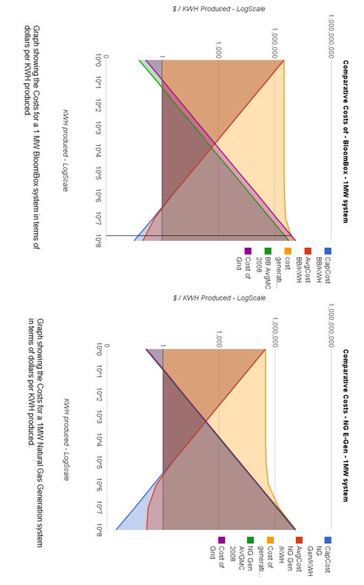
Table of Contents
    Introduction
    The Science of a Fuel Cell
        Technical Advantages of Solid Oxide Fuel Cells
        Obstacles and Current Research
        Summary of Technology Status
    Commercial Applications of Solid Oxide Fuel Cells
        Delphi Automotive SOFC APU
        Bloom Energy
        Ceres Power
    The Natural Gas Market
            Natural Gas Consumption in California
            Natural Gas Price Forecasts
                California Energy Commission: 2007 Natural Gas Market Assessment, Final
                Staff Report
                Energy Information Administration Annual Energy Outlook 2009 Forecast
                California Public Utilities Commission, Market Price Referent 2008
                California Energy Commission 2007 Scenario Analysis Project—Case 2—
                High Sustained Natural Gas and Coal Prices
    Benefit-Cost Analysis
        Assumptions in our Calculations
            Discount rate
            Time-frame
        Private Benefits and Costs
            BloomBox Technical Specifications and Price Sensitivities
            Reliability
        Social Benefits and Costs
            Reduced Carbon Dioxide Emissions From Bypassing Power Grid
            Reduced Availability of Rare Metals
    Conclusions
    References
    Appendix
        Natural Gas Market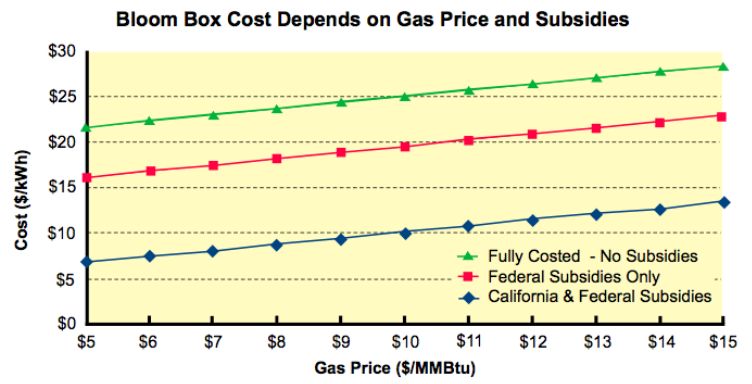
Introduction
Solid Oxide Fuel Cells (SOFCs hereafter) can provide a wide range of benefits to users for
the purpose of electricity generation. In the research we will carry out, we aim to address the
question of whether both federal and state policies and the economics specific to SOFCs
make them economically viable. We will focus on a particular commercial application of
SOFCs, namely the BloomBox. In order to restrain the extent of our analysis, we will also not
consider the use of BloomBoxes as a combined heat and power (CHP) unit, since, while this is
technically possible, it is far from a common practice, especially in a state such as California,
where heating is not a primary concern or one of the primary consumers of energy .

The electricity grid that supplies retail customers in the California, as well as the wider United
States, is becoming increasingly burdened with the greater demands placed on it through
increased energy consumption as well as the aging of the infrastructure currently in place. In
this paper, we will consider the feasibility BloomBoxes, and their potential in helping California
meet its energy demands. SOFCs, first developed in NASA’s Apollo program, have three
qualities that make them attractive as a source of energy in the future:
    1. They operate independently of the transmission grid, instead being installed in the
        homes or offices they are electrifying, so are immune from the inefficiencies inherent in
        distributing electricity over large distances;
    2. The waste heat from the generation process can be used either to heat water or for
        space heating, increasing the overall efficiency of the units;
    3. Since the energy is made electrochemically the fuel cells are far more efficient at
        generating energy than any source that relies on the burning of fuel.
Despite the benefits of using SOFCs as a source of energy, there are also costs associated with
them, including the high cost of initial installation and the problems of manufacturing fuel for
the cells, that need to be considered before reaching a conclusion as to whether SOFCs are a
viable source of energy that can form a significant portion of the California’s energy mix.

At present, fuel cells are already competing with existing technologies in three different, broad
markets (stationary power, automotive, and portable and equipment markets), and within
each group there are a wide range of applications. This paper, however, will concentrate
on BloomBoxes and their use as a source for generating power in the state of California
(discounting combined heat and power systems since heating systems are of relatively little
importance to overall energy consumption in California).

In 2007, California produced 69.5% of the electricity it uses; the rest is imported from the Pacific
Northwest (8.2%) and the U.S. desert southwest (22.3%). Natural gas is the main source for
electricity at 45.2% of the total system power. In 2005, Californians spent $31 billion for their
electricity (The California Energy Commission, 2010).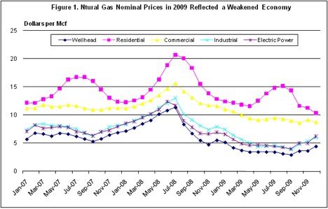
The Science of a Fuel Cell
In order to understand the role that SOFCs may play in the future, it is first essential to
understand the science behind the operation of a SOFC in terms of the technology’s potential
and limitations. In principle, the operation of a fuel cell can be explained as an electrochemical
reaction. The basic components of a fuel cell are the anode, cathode, electrolyte, and a wire. A
simple illustration is shown in figure 1. In introductory Chemistry courses, a common phrase
is “LEO says GIR.” This phrase is the key to understanding the chemical reactions that occur in
a general fuel cell. The phrase stands for, “losing electrons is oxidation, and gaining electrons is
reduction.” Hence, in a reaction in which an element loses electrons, the element is said to be
oxidized, or an element gaining electrons is reduced. In simplest terms, the anode is the site at
which oxidation takes place in a fuel cell. Conversely, the cathode is the site at which reduction
takes place. Specifically, the reduction reaction that occurs at the cathode in an SOFC can be
written as: O2 + 4e-     2O-2. The electrolyte is a substance that allows ions such as O-2 to
migrate between the cathode and anode due to vacancies in the lattice of the ceramic at the
atomic level (Ref 1). In a SOFC, the electrolyte is a non-conducting ceramic material that
performs well when heated to 750 to 10000C(Ref 1). At the anode, the oxidation reactions that
occur are: H2 +O-2        H2O + 2e- as well as CO + O-2     CO2 + 2e-. Finally, there is a build up
of electrons at the anode due to oxidation and a shortage of electrons for further reduction at the
cathode. Hence, we can link the anode to the cathode via a wire as shown in figure 1. Electrons
will flow through the wire due to the spontaneous oxidation and reduction reactions at the anode
and cathode respectively. Electrons are said to be traveling down a potential gradient. This is
similar to a ball rolling down a hill. Although a SOFC can run on a variety of hydrocarbon fuels
including methane, the hydrocarbon fuels are catalytically reformed so that the gases flowing
into a SOFC are CO, H2, and O2. The overall reaction in the SOFC is: H2 + CO+ O2         H2O +
CO2 + energy. Here, energy takes the form of a potential that drives the flow of electrons as well
as heat that warms the exhaust as well as the fuel cell itself. Within a SOFC, many individual
fuel cells are connected together via a conducting ceramic material called an interconnect
(Ormerod, 2003).

Fig 1. A basic design for a solid oxide fuel cell
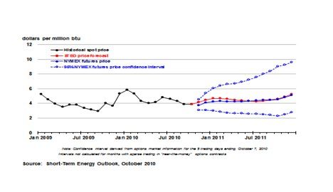
Fig. 2 A prototype planar solid oxide fuel cell stack (Ormerod, 2003)

Technical Advantages of Solid Oxide Fuel Cells
SOFCs present several technical advantages over conventional power plants. These
advantages include lower emissions of sulfur oxides, nitrogen oxides, and CO2 per watt.
Potentially, SOFCs are reliable with very little maintenance, and there is potential for
applications of SOFCs in applications where power must be uninterrupted such as sensitive
electronics or life-supporting equipment (Ormerod, 2003). Additionally, with the advance of
carbon capture technology, it could become practical to capture the CO2 leaving a SOFC. In
addition, SOFCs can theoretically reach 80% energy efficiency when the exhaust is run through
gas turbines, and they can quietly generate electricity at the site where electricity is required,
which avoids inefficiencies and expenses associated with transmitting power from a central
power plant to a consumer. This is especially valuable in remote locations and locations that
suffer from inadequate electrical generating capacity. Furthermore, SOFCs can operate on
a variety of hydrocarbon fuels such as natural gas, which is already distributed throughout
many developed countries, and biogas, which is a potential renewable hydrocarbon fuel.
In many cases, the waste heat of the exhaust can be used for heating purposes instead of
running a turbine to produce more electricity. Thus, SOFCs could be the basis for combined
heat and power systems for modern buildings. Furthermore, electricity production can scale to
applications where only a few watts are required to megawatts. Water use within a fuel cell is
estimated to be 1% to 2% of the water use of a household. Furthermore, the high power density
of SOFCs combined with the potential for low emissions has made SOFCs a subject of interest
for generating electricity in vehicles potentially to drive the car or to only operate electronics
(Ormerod, 2003).

Obstacles and Current Research
Nevertheless, although SOFCs have existed for over the last 160 years, SOFC research
stalled until the 1960’s because the high temperature of fuel cell as well as the harsh
reducing environment created by the gas used as fuel has lead to serious issues in terms
of finding suitable materials to construct an efficient fuel cell (Ormerod, 2003). Electrolytes,
anodes, cathodes, and interconnects must be able to tolerate harsh conditions. Furthermore,

these ceramic fuel cells are prone to damage during start up and shutdown of the system
because ceramics undergo thermal expansion, but they are relatively poor conductors of
heat. Consequently, during a warm up or cool down the brittle ceramics will not have uniform
expansion and contraction, which causes cracking of the ceramics and failure of the cell.
Therefore, current SOFCs are unsuitable for intermittent production of electricity. This limitation
has hindered the use of SOFCs in transport applications, which often means rapid cooling and
heating of the brittle ceramics. Furthermore, it prevents solid oxide fuel cells from increasing
output to follow load demands from a household throughout the day. A household running a
SOFC must run either independently from the grid, in parallel with the grid, or it must be run in
some combination. A system independent from the grid must use an expensive battery system
or limit energy consumed (McClelland and Torro, 2002). A system running in parallel with the
grid will either draw power from the grid or put electricity on the grid depending on household
electricity use while a combination system will cut itself off from the grid in the event of a power
outage. Each option requires expensive electronics (McClelland and Torro, 2002). In terms of
estimated costs, assuming maintenance once per year and an operating life of 10 years, the
cost of labor, piping assembly, materials, electronics, insulation, natural gas, reformer, and heat
exchanger could bring a SOFC system as high as 30 cents per watt of capacity according to
some existing designs (DOE NTEL, 2002). Furthermore, because of the relatively small size of
2-5 kilowatt systems companies are unlikely to achieve economies of scale without producing
devices in mass quantities (McClelland and Torro, 2002). However, despite technical limitations
mentioned in this section, SOFC systems have been reported that last on the scale of years in
lab settings (Halinen, Saarinen, Noponen, Vinke, Kiviaho, 2010).

Another limitation of an SOFC system is that energy is lost when the DC current produced by
the SOFC must be converted to the 60 Hz AC current required by most appliances. Additionally,
thick electrolytes ceramic cause resistance to ion transport. Since the 1960’s, research into
SOFCs has focused on planar and tubular designs as well as new electrolyte materials that
would enable greater efficiency, durability, and lower operating temperatures. In addition,
research has also focused on internally reforming hydrocarbon fuels inside the SOFC instead
of within an external reformer. This would make SOFCs more economical in that they would
simplify the system. However, internal reforming means exposing the anode to sulfur impurities
and solid carbon deposition, which poison the anode’s ability to function.

Zirconium oxide doped with ytterbium oxide has been found to be an effective electrolyte
material because conducts O-2 ions and can tolerate an oxidizing and reducing atmosphere
(Ref 1). While the costs of pure ytterbium oxide are prohibitively expensive, zirconium oxide
is relatively cheap, abundant, strong, electrically insulating, and easy to fabricate (Ormerod,
2003). Other oxides such as scandium oxide and calcium oxide have been used as dopants
to zirconium oxide, but ytterbium oxide is generally considered superior for reasons of cost,
availability, and stability (Ormerod, 2003). While the operating temperature of a fuel cell is
dictated by the electrolyte thickness and ionic conductivity, operating the solid oxide fuel cell
below 7000C would enable cheaper materials to be used in the fuel cell to produce power at
high efficiencies (Ormerod, 2003). Hence research on this front has investigated a variety of
electrolyte materials as well as designs for thinner electrolytes, which must be supported by
other structures such as the anode or cathode. Currently, consistent thicknesses on the order of
10 micrometers have been obtained (Ormerod, 2003).

Other electrolytes that have shown promise include gadolinia-doped ceria and lanthanum
gallate. Unfortunately, gadolinia doped ceria forms Ce+3 at high temperatures, which conducts
electrons and prevents them from traveling through the interconnect. At temperatures below
5000C, the electrolyte is has a sufficient ionic conductivity, but current cathode materials are
not active enough to turn O2 into O-2 at a fast rate. Lanthanum gallate does not possess these
problems, but its chemical structure changes with temperature, which makes the ceramic
electrolyte dramatically more brittle.

In terms of anode composition, the metal used for an anode must resist oxidation under
operating conditions, which limits the potential metals to cobalt, nickel, and precious metals. As
a result, nickel is a popular anode choice because it is the cheapest, and it is used to make a
porous anode by mixing its dust with electrolyte to form a mixture to join to the electrolyte, but
this process is complicated by the thermal expansion mismatch between the electrolyte and the
nickel (Ormerod, 2003). Research has experimented with adding a third material to this mixture
or replacing the anode with an electrically conducting oxide in an effort to improve internal
reforming, reduce carbon deposition, and reduce poisoning of the fuel cell with sulfur, which is
present in hydrocarbon fuels in trace amounts (Ormerod, 2003).

Additionally, the cathode must also be robust enough to tolerate harsh chemical conditions
while being porous and electrically conductive, which limits the choices of material to rare
metals or conducting oxides with thermal expansion coefficients close to the electrolyte ceramic.
Zirconium oxide SOFCs generally use LaMnO3 doped with strontium. However, temperatures
over 13000C cause manganese to diffuse into the electrolyte, which impairs fuel cell operation
(Ormerod, 2003).

The interconnect must be able to tolerate reducing and oxidizing atmospheres while conducting
electricity and preventing the mixing of gases at the anode and cathode. A canonical choice of
material for this role is LaCrO3. Although this material conducts 1000 times better in air than in a
hydrogen atmosphere, the conductivity of LaCrO3 does not limit performance in current designs
(Ormerod, 2003). However, at lower temperatures, it would be feasible to use cheaper materials
such as stainless steel composites.

Summary of Technology Status
Overall, much research is required for SOFCs to realize their potential as an efficient and widely
desirable means of producing electricity. However, SOFCs have already been shown to be
beneficial and attractive for a range of applications. This technology has also been shown to be
feasible in a lab setting. Although there is tremendous room for improvement in terms of cost,
durability, and efficiency, this technology is ready to produce electricity outside of a lab setting.
Commercial Applications of Solid Oxide Fuel Cells
In the last few years of the origination of methane fuel cells, or solid oxide fuel cells (SOFC),
we have seen much growth in the industrial development of this technology. The technology’s
mobility and minimal maintenance requirements, coupled with relatively low costs, lends itself to
numerous industrial utilizations. Thus, there have been many applications of SOFC technology
coming to fruition in competitive markets for electricity generation.

Delphi Automotive SOFC APU
In a joint venture with BMW, Delphi Automative has been developing solid oxide fuel cells for
commercial vehicles since 1998. The venture has provided major leaps, particularly in the
area of stationary power management. The venture has allowed to produce onto the market
a a Solid Oxide Fuel Cell (SOFC) Auxiliary Power Unit (APU), producing 5kW of electricity
via electrochemical generation. As the fuel converts electricity without combustion, the Delphi
SOFC APU operates at higher efficiency levels than previous traditional internal combustion
engines, while further eliminating pollutants and noise (Delphi, 2010)

The SOFC APU application of this product has proven to be particularly useful in the
transportation industry where this technology can provide an auxiliary power supply, allowing
the truck operator access to cab accessories such as “cab lights, refrigerators, microwave
ovens, and audio systems” without having to turn on the primary engine or leave it idling. Delphi
estimates that the SOFC APU could “save up to 85% of the fuel now required for the operation
of the main diesel engine during idling” (Delphi Website, 2010). As seen in the picture (Delphi
Website, 2010) below, the Delphi SOFC APU is quite small and is not space intensive.

The partnership between Delphi and BMW has allowed BMW to also implement the technology
in their sedans, complimenting the main combustion engine, while reducing variable costs.

Bloom Energy
The most prominent modern application of the solid oxide fuel cells is the “Bloom Box” whose
history stems from Dr. K. R. Sridhar’s research group for the NASA Mars exploration program.
The group was looking to develop a sustainable, yet efficient, energy source at the Space
Technologies Laboratory at the University of Arizona, but later moved on to form the current
company, Bloom Energy in 2001-2002, after securing funding from a few venture capital firms
(Bloom Energy Website, 2010).

The latest Bloom Box model, the Bloom Energy ES-5000 which can intake natural gas,
hydrogen, or even garbage dump gas costs $700,000-800,000 (Bloomberg, 2010). It is capable
of generating 100kW, enough electricity for approximately 100 homes. Since its entrance
into the market in July 2008, it has been bought several Fortune 500 firms including Google,
Staples, Walmart, FedEx, Coca-Cola, and Bank of America (Bloom Energy Website, 2010).
Its proven reliability and economic efficiency has been shown in eBay’s decision to use this
SOFC fuel source in generating 15% of the electricity consumed in its main San Jose, California
headquarters (Christian Science Monitor, 2010). Such widespread use of this product is no
mistake as it is highly economical, generating electricity at 8 to 10 cents a kilowatt hour, albeit
with subsidies from the state of California, much lower than the usual commercial cost of
electricity at 14 cents/kilowatt hour (New York Times, 2010).

This seemingly miraculous technology does comes with a few disadvantages and hurdles
however. Besides the high upfront capital costs, solid oxide fuel cells also relies on extremely
high operating temperatures, around 800-1000 degrees Celsius. As a result, Bloom Boxes
may be vulnerable to breaking down if not managed and serviced properly. Furthermore, this
technology requires a slow startup as it needs to heat up to the high operating temperature
before being able to fully run (Scientific American, 2010). Most of the dangers of such a high
operating temperature are harnessed, but it still causes some hindrances when it comes to
efficient operation.

Ceres Power
While the disadvantages of the Bloom Box is the high temperature, there have been competitors
such as Ceres Power looking to capitalize on this weakness and develop an improved solid
oxide fuel cell with lower operating temperatures. By replacing the original anode material,
yttria stabilized zirconia (YSZ,) with cerium gadolinium oxide (CGO), Ceres has been able to
reduce the operating temperature from 800-1000 degrees Celsius to 500-600 degrees Celsius.
This significant reduction in temperature allows the electrochemical layers to be thinner, and
improving performance, while reducing material costs. Additional advantages to Ceres Power’s
development also include thermal shock resistance, fast start-up times, and more mobility
(Ceres Power, 2010).

A common thread that we have seen in the application of solid oxide fuel cells technology
brought onto the market is that it is competing in highly competitive markets. The versatility of
this product to be used from commercial and residential electricity generation to automobile
auxiliary power proves the extent to which such a powerful technology can be applied.
SOFC technology’s impact in the future is imminent when costs eventually lower from further
improvements in research and development, allowing it to beat alternatives with higher costs.
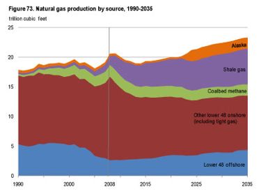
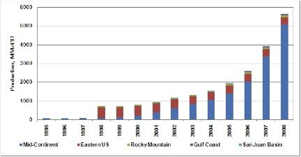
The Natural Gas Market
The primary fuel for the solid oxide fuel cell is methane, which is the main constituent of natural
gas. According to the Bloom Energy website, the ES-5000 Energy Server consumes 0.661
MMBtu/hr of natural gas to produce 100 kW of electricity. A cubic foot of natural gas produces
approximately 1000 Btu’s, so the ES-5000 Energy Server consumes natural gas at the rate
of approximately 661 cu. ft. per hour. To put that number in some perspective, according to
2008 figures from the American Gas Association, the average household in the U.S. consumes
approximately 9 cu. ft. of natural gas per hour for heating and cooking. The Bloom ES-5000
Energy Server consumes approximately as much natural gas to produce 100 kW of electricity
as 73 homes consume on average for heating and cooking.

Because natural gas is the primary fuel for solid oxide fuel cells, the commercial viability of the
technology depends in part on the price of natural gas. Price projections for any market priced
commodity are speculative by nature. For natural gas, future prices are complicated by price
variations between geographic regions and by retail prices which vary depending on the size of
the customer. Wholesale electricity generators pay less per cubic foot than households.

Demand for natural gas as a fuel for electric power generation has grown slowly but steadily
for the past twenty years. It is an attractive fuel for electric power because it is clean burning
and efficient, and because ample supplies of natural gas have been available from domestic
resources and from Canada. In fact, the vast majority of new electricity generation capacity built
in the United States in the past decade has been natural gas-fired.

The most dramatic long-term factor in the U.S. natural gas market is the discovery of vast
domestic reserves of natural gas from unconventional sources including deep-well gas, coalbed
methane, tight sands gas, and most importantly, shale gas. The most significant trend in U.S.
natural gas production is the rapid rise in production from shale formations. In large measure
this is attributable to advances in the use of horizontal drilling and well stimulation technologies
and refinement. Hydraulic fracturing – the high pressure injection of water, sand and chemical
lubricants into underground shale formations - is the most significant of these technologies. A
few years ago, most analysts foresaw a growing U.S. reliance on imported sources of natural
gas, and significant investments were being made in regasification facilities for imports of
liquefied natural gas (LNG), according to the Energy Information Administration (EIA).

How shale gas will affect future prices is uncertain. Shale gas is more expensive to produce
than natural gas from traditional underground reservoirs. Furthermore, there may be technical
or environmental factors that might dampen shale gas development, but analysts agree that the
potential supply is enormous.

The boom in natural gas from shale formations began in the mid-1990s. At that time, shale
deposited natural gas provided about 1 percent of the Lower 48 production. By 2008, however,
the shale production rose to occupy almost 10 percent of production from the Lower 48.
According to the Natural Gas Supply Association, production from shale could double in the
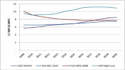
next 10 years and provide one-quarter of the nation’s natural gas supply. The EIA's Annual
Energy Outlook 2010 predicts that total domestic natural gas production will grow from 20.6
trillion cubic feet in 2008 to 23.3 trillion cubic feet in 2035. With technology improvements and
rising natural gas prices, natural gas production from shale formations is predicted to grow to 6
trillion cubic feet in 2035, more than offsetting declines in other production. In 2035, shale gas
is estimated to provide 24 percent of the natural gas consumed in the United States, up from
just 6 percent in 2008.

Natural Gas Consumption in California
According to the California Energy Commission, natural gas demand for the electric power
sector in California is expected to increase by 2.4 percent over the next decade, while overall
gas demand in all sectors is forecast to increase slightly higher than 1 percent annually. Some
contributing factors to this slower growth in overall demand are: (1) increased use of renewable
energy; (2) slower growth rate in electric generating capacity; (3) more fuel-efficient natural gas
power plants; (4) flat growth in the industrial sector; (5) improved efficiency requirements for
buildings and appliances through standards; and (6) new demand-side management programs.
This slow growth in demand bodes well for natural gas prices in California.

Natural Gas Price Forecasts
Source: California Energy Commission
The above figure compares four Henry Hub natural gas spot price forecasts through the
year 2020: (1) California Energy Commission’s 2007 Final Natural Gas Market Assessment
(2007 NGMA) prepared in support of the 2007 Integrated Energy Policy Report, Energy
Information Administration’s Annual Energy; (2) Outlook 2009 (EIA AEO 2009); (3) Energy
Commission Scenario Analysis Project Case 2 (SAP High Case); and (4) California Public
Utilities Commission (CPUC) Market Price Referent (CPUC MPR 2008).

California Energy Commission: 2007 Natural Gas Market Assessment, Final Staff Report
This model predicts an upward trend in natural gas prices to about $6.50 per million cubic feet
in 2020. The 2007 NGMA natural gas price forecast was produced using the Market Point,
Inc., World Gas Trade Model (WGTM)/ North American Regional Gas (NARG) component,
produced as part of a natural gas market assessment, and in support of the Energy Commission
2007 IEPR. The WGTM is a generalized, equilibrium model that produces market-clearing
natural gas wholesale prices, quantities, natural gas production, and pipeline flows at a market
equilibrium of supply and demand. The model simulates the physical structure of the market,
accounting for expected market changes.

Energy Information Administration Annual Energy Outlook 2009 Forecast
This model predicts a slight upward trend in natural gas prices leading to a price of about
$7.50 per million cubic feet in 2020. The EIA AEO 2009 forecast was produced using the
National Energy Modeling System (NEMS). This annual forecast is widely used by analysts,
planners, and decision makers inside and outside government for study, analysis, planning,
and investment decisions. NEMS contains separate modules for regional fuel markets and
consumer sectors (i.e. industrial, commercial and residential), as well as macroeconomic and
international modules. The model balances supply and demand for each of the fuel markets,
while accounting for competition between different fuels.

California Public Utilities Commission, Market Price Referent 2008
This model, based on NYMEX natural gas forward contract prices predicts a declining trend in
natural gas prices to just under $8 per million cubic feet in 2020. In accordance with California’s
Renewables Portfolio Standards Program, the CPUC develops a natural gas price forecast
(CPUC MPR 2008) to establish an avoided electricity cost benchmark, the Market Price
Referent (MPR) for non-renewable energy. The MPR then serves as a benchmark to evaluate
the reasonableness of the prices paid by investor-owned utilities for renewable energy.
California Energy Commission 2007 Scenario Analysis Project—Case 2—High Sustained
Natural Gas and Coal Prices
This is the high price scenario assuming a decline in domestic production over the next ten
years. It puts natural gas prices at close to $11 per million cubic feet in 2020. The Scenario
Analysis Project, prepared in support of the California Energy Commission 2007 IEPR, was
designed to provide a greater understanding of the implications of various levels of market
penetration of “preferred resources,” such as energy efficiency measures and renewable
electricity generation, in both California and the Western states. In support of developing
one scenario, SAP Case 2, the High Sustained Natural Gas and Coal Prices, Global Energy
Decisions’ Gas Pipeline Competition Model (GPCM), which allows users flexibility in analytical
structure, was used to forecast gas prices that potentially could result from a prolonged scarcity
of domestic natural gas supply. Major GPCM assumptions for this scenario included:
● Domestic natural gas production declines between 12 to 32 percent over the forecast
period.
● Neither the Alaska North Slope nor MacKenzie Gas Project pipelines are constructed
during the forecast period.
● LNG imports increase, supplanting the declining domestic supply.
● High oil prices and a closer correlation between oil and natural gas prices would result
if climate change regulatory policies accelerate the use of natural gas for electric
generation.
The current December 2010 New York Mercantile Exchange (NYMEX) price for natural gas is
$4.03 per million cubic feet. January 2020 natural gas futures contracts are currently trading
on the NYMEX at a price of $6.98. The mean 2020 projection of the NYMEX price and the
four models described above is approximately $8 per million cubic feet. If we discard the
California Energy Commission high price scenario model, the mean forecast price for 2020 is
approximately $7.25.
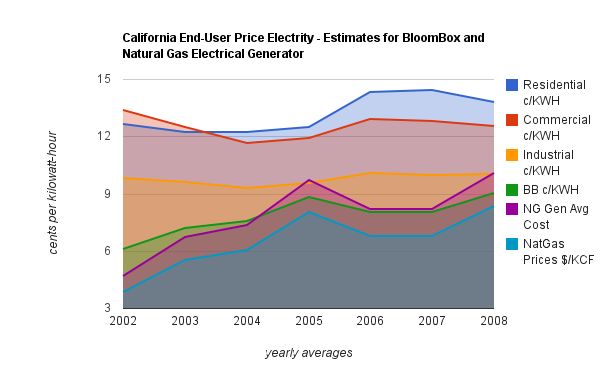
The figure below illustrates short-term forecasts through 2012 with a NYMEX futures price 95%
confidence interval roughly between $3 and $10.The following graph shows the impact of gas price on the over cost ($/kWh) of energy produced by the BloomBox, as well as the impact of federal and California state subsidies on the price.
Benefit-Cost Analysis
Assumptions in our Calculations
Discount rate
We chose a discount rate of 7%. This figure is based on using a methodology based on rate of
return on private investment. The Office of Management and Budget (U.S. government agency)
states:
        “Base-Case Analysis. Constant-dollar benefit-cost analyses of proposed investments
        and regulations should report net present value and other outcomes determined using a
        real discount rate of 7 percent. This rate approximates the marginal pretax rate of return
        on an average investment in the private sector in recent years. Significant changes in
        this rate will be reflected in future updates of this Circular” (Office of Management and
        Budget, 2009).

Time-frame
The time-frame for the analysis is based on the predicted lifespan of BloomBox of 10 years, and
we will calculate levelized costs across this 10 year time-frame.

Private Benefits and Costs
BloomBox Technical Specifications and Price Sensitivities

The above graph, shows the projected cost of generating capacity of solid-oxide fuel cells
(of which BloomBoxes are one type) relative to other energy sources. What is clear from the
diagram is the following:
● The obvious problem with fuel cells is that they require the end-user to pay a large fixed
cost in order for the unit to be installed, despite the subsidies they have
● Fuel cells are clearly more economically feasible for larger consumers of energy (i.e.
office buildings rather than typical family households)
● Surprisingly, SOFCs can compete with pulverized coal as a cost-effective fuel for
generating capacity, given large plant size, although this is dependent on a necessarily
low gas price level (Seattle, Washington is an example of high gas price levels
preventing SOFC being efficient, according to City of Seattle, 2010)
Looking at the costs of operating a Methane Fueled Solid Oxide Fuel Cell (M-SOFC), the two
immediately noted costs are the fuel stock (Natural Gas) and the up-front capital costs of the
system. Other costs such as maintenance, financing and insurance can be factored with the
capital cost (including and fuel cost into an average cost of the system).
A M-SOFC like the BloomBox consumes 660,000 BTUs of natural gas in an hour to produce
100KW of electricity (Bloom Energy, 2010). For natural gas, there is approximately 1000 BTU's
per 1 cubic foot. Natural gas prices are quoted using 1000 cubic feet (KCF), so a device like the
BloomBox consumes 0.66 KCF per 100 kiloWatt-hours (KWH) of electricity produced. To find
the cost of each individual KWH, the price of natural gas times the consumption of the device,
then divided by the output will give the marginal price of that unit of electrical energy. Here, the
price of gas times 0.0066 will give the cost of each additional KWH produced. Because the price
of natural gas fluctuates daily as producers, retailers, and consumers negotiate prices over
different periods, finding an “average” marginal cost of cast will be based on projections of the
gas market, and the certainty of those fluctuations. For 2008, an average cost for 1000 cubic
feet of natural gas in California was $8.34, which at that price would yield a price of 5.5 cents
per KWH. But this is not the complete picture.
Tallying the price-tag of the system with additional costs such as initial set-up costs, financing,
and maintenance, with deductions for direct subsidies and/or tax-rebates will give a system
cost (not the cost of operating the system). The system will have some life-time over which
it operates, in this case hours of electrical generation. Taking the cost of the system divided
by the product of the hourly generation capacity by the total number of hours the system
is expected to run will yield a production capacity cost for the the system. By adding the
production capacity cost of the system to the marginal cost, an average cost value is found.
In the BloomBox example, the capital cost per unit is advertised at $800,000 for a 100KW
generation capacity. Cost of financing the system is difficult to ascertain, as different
organizations will have different funds available to them as to what loans, if any, and what
interest they will pay. Maintenance costs are unknown, but can be explored through assumed
annual rates. Financing, insurance and scheduled maintenance (and average projected
unscheduled maintenance) and other yearly costs discounted and added as upfront costs cangive a present value of the system. Subsidies as tax-breaks, tax-rebates, or direct subsidies can be deducted from the the up front cost of the system (or deducted and discounted for when the purchaser of a such a system is given the subsidy). The Federal Business Energy Investment Tax Credit covers 30% of the cost of a fuel cell system, up to $1,500 per 0.5 KW of generating capacity (DSIRE, 2010) (or $3,000,000 per MW), and the state of California has a $2.50 / Watt of generation capacity incentive for fuel cells that consume natural gas (Center for Sustainable Energy California, 2010) up to 1MW generation capacity, although a system that is fed from renewable fuels receives an incentive of $4.50 / Watt generation capacity (again, up to 1MW). These additional incentive to Businesses in California maybe the primary reason why many companies in California are purchasing these systems. To maximize the subsidy for this system, a company may wish to purchase the maximum amount covered by the subsidies, which in California is 1MW of generating capacity. A 1MW BloomBox system has a capital cost of $8,000,000, a federal subsidy of $2,400,000, a California subsidy of $2,500,000. Before maintenance and financing, the cost of a 1MW Bloom system is down to $3,100,00, generating 87,660,000 KWH of energy (8766 hours/year, 100KW per hour per unit, 10 units in system, over the proposed 10 year life span of the system) (Woody, 2010), bringing the production capacity cost of such a system to around 3.5 cents/KWH, or $35 per MWH. Without these subsidies, that capacity cost 9.13 cents per kiloWatt hour ($91 per MWH). Adding then the Marginal Cost of the Fuel Consumption (5.5 cents/KWH) with the production capacity cost (3.5 cents/ KWH for the purchase of the system, not including maintenance, financing or insurance) does one see the cost of a 1MW system in California at 9 cents/KWH. In comparison with drawing electricity from the electrical grid system, where the average price for commercial users of electirity was 12.54 cents /KWH. The 3.5 cents/ KWH price difference would lead to a savings of $616,000 in one year. With a discount rate of 7%, 10 years of using the 1MW system at these prices for natural gas ($8.34/KCF) and the commercial price of electricity ($12.54), the savings between drawing from the grid and using the BloomBox would pay for the BloomBox system in just over 5 years, with the remaining lifetime of the system returning $2,300,000. However, this positive return on the BloomBox is only applicable with the extant price supports and these price levels. If California were to repeal this incentive, the production capacity cost would raise 6.3 cents / KWH, with an average cost of 11.9 cents /KWH, making the pay-back period on a BloomBox 9.1 years, yielding a savings of $420,000 (before maintenance, financing, and insurance). With no price supports, the BloomBox has a 13 year pay-back period, 3 years longer than the expected system lifetime, at a cost of $1,400,000 over that of using the same amount of electricity from the grid. If there were a greater difference between the price of natural gas and the commercial price of electricity, or if the BloomBox had technical improvements in its fuel economy or if there were a reduction in its purchase price, then that payback period could be reduced for the system to not be a net expense. For example, at the prices for natural gas and commercial electricity used above, the 1MW BloomBox system would need a purchase price of $6,160,096 ($616,010 per BloomBox unit).
As a comparison, a non-subsidized system of 10 piston-driven reciprocating type 100 KW
natural gas fed electric generators, price tag $30,000 per generator (Norwall PowerSystems,
2010 and Generac Power Systems, 2009) (for $300,000 purchase price) has a production
capacity cost of 0.34 cents /KWH, but consumes fuel at approximately twice the rate of the
BloomBox (making the marginal cost of consumption 1.34/100 times the price of natural gas).
At the same prices used above for gas and electricity with the M-SOFC, the average cost
is 11.5 cents /KWH, but because of the low initial capital cost, this system has a 2.5 year
payback period. However, because of the high average cost (mostly due to the 11.1 cents /
KWH marginal cost of generation) the system would save $680,000 over 10 years (discounted
at 7%) compared to the purchasing the same amount of power from the grid, prices staying
unchanged. For a BloomBox to have a similar savings with no price supports, it's initial price
would be $5,256,750 for the 1 MW system ($525,675 per unit).
Although these analyses have been done using static prices for electricity and natural gas,
allowing for variations in price based on projection scenarios compiled by the U.S. Energy
Information Administration, the value of these systems can be seen over their projected time of
usage. Using national projections from the Annual Energy Outlook 2010 (by the USEIA), there
are two scenarios that illustrate the how beliefs in future prices may influence a decision to
purchase such a electrical generation system. Electricity prices are projected in terms of a
baseline reference estimation, with a range given around that allowing for strong or weak
economic growth (US Energy Information Administration, 2010a). Natural gas prices are given
around a baseline with the range determined by high or low oil prices (US Energy Information
Administration, 2010b). Using the opposite ends of electricity/natural gas prices can be used to
find the maximum and minimum projected differences of the system. Projecting prices for
California's by using historic price differences with data collected from EIA for the prices of
Natural Gas used in electricity generation (being more expensive in California by a factor of
1.43), and the commercial price of electricity (more expensive by a factor of 1.39), the extreme
projected scenarios show that using a BloomBox in California can be as much $3,150,000 in a
strong growth economy with low oil prices, or $2,170,000 in a weak growth economy with high
oil prices (both figures discounted at 7% over a 10 year period from 2011 to 2020, not including
maintenance, financing or insurance costs, in 2009 dollars). Comparatively, a natural gas-fed
conventional combustion electrical generator in a high growth, low oil price scenario would cost
$2,300,000 less than purchasing the same amount of power from the grid at projected
commercial rates, and in a low growth, high oil price scenario would be $700,000 less than the
grid (again, discounted at 7% between 2011 and 2020, not including maintenance, financing and
insurance, at 2009 USD). Compared to the 2009 static prices for natural gas and commercial
electricity, the current projections favor the use of a BloomBox for power generation over the
grid at the 1 megawatt scale in California.

Reliability
Given that BloomBoxes by-pass the grid and are not susceptible to outages caused by adverse
weather conditions, they will benefit the user by providing a reliable source of energy. However,
given the wide variation is reliability across the state of California, this study will not try to
quantify the benefit of increased reliability.

Social Benefits and Costs
Reduced Carbon Dioxide Emissions From Bypassing Power Grid
The graph below shows the scope of decentralized generation as a market for power
generation. While it illustrates decentralized generation has a wide range or potential
applications, high temperature fuel cells such as SOFC tend to be “less flexible, thereby
particularly suiting larger-scale base-load applications” (Avadikyan, Cohendet, & Heraud, 2003:
61).
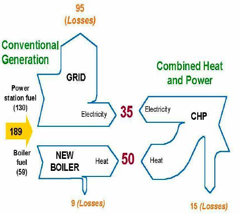
While the below figure was designed to illustrate the efficiencies of a Combined Heat and Power
(CHP) system over a conventional power generation and supply, it is nonetheless abundantly
relevant to the use of BloomBoxes in California, since, like CHP system, they bypass the
grid. Given that we are only considering the use of SOFC to provide power, and not heat, the
benefits we will consider will be somewhat less than the below diagram outlines, but since the
vast majority of power use in California is not used to heat, there will still be huge efficiencies in
the adoption of SOFC, including BloomBoxes, as a source of power.
If we put a carbon price of $13.70 per tonne of carbon dioxide emitted, we would be able to
quantify the benefits of reduced emissions as a result of the use of BloomBoxes to supply power
without the use of the inefficient grid system. This price was chosen since it is the price put
on carbon dioxide under the cap-and-trade system proposed by President Obama (Business
Green, 2009). I will also use a lower estimate and upper estimate for carbon prices to give a
range to the varying degrees of decentralization of energy production that might occur.

As we can see from the diagram, only around 35 of the 130 units (27%) of energy generated
at the power plant reaches the end user; since we know California generated 490 MMT
(million metric tonnes) of CO2 emissions for in-state electricity generation in 1990 (California
Environmental Protection Agency, 2007), we can thus calculate the emissions stemming from
the electricity lost in transmission:

%power lost in transmission x total emissions from power generation x carbon price

.73 x 49,000,000 x 11 = 393,470,000
.73 x 49,000,000 x 13.7 = 490,049,000
.73 x 49,000,000 x 15 = 536,550,000

The following table is based from these calculations. However, since it is unthinkable that
California will dispense with the need for a transmission grid in the near future, the table outlines
the varying degrees of benefits based on the varying price of carbon and the percentage of
energy bypassing the grid.

Benefits from reduced emissions over one year period based on 1990 emissions figures (since
we were not able to find more recent figures pertaining to emissions resulting from power
transmission) and carbon prices in the year 2009:

Benefits depending on degree of decentralization over one-year period based on 1990
emissions figures:

The above table shows the increasing benefits seen when more energy is supplied via on-site
methods. On one extreme, if all energy in California bypasses the grid and is generated at the
point it is consumed, and we take the upper estimate carbon price, we would see the benefits
of reduced carbon emissions over a one-year period at $536,550,000 (in 2009 dollars), which
would certainly help California ameliorate its current budgetary predicament.

If 5% less energy than the total amount of energy transmitted by California’s power grid in 1990
was transmitted, than, given the range of carbon prices outlined above, we can calculate the
annual average benefits in 2009 dollars using a discount rate of 7%. As the below table shows,
if energy transmitted over the grid decreases 5%, then the annual benefits of the reduced
emissions of carbon dioxide range from $22,651,491 to $27,388,274.

Benefits of reduce emissions if BloomBoxes reduce power sent over grid by 5%:

Since earlier analyses use the predicted and advertised lifespan of a BloomBox, 10 years, to
calculate the benefits of reduced carbon dioxide emissions would likewise seem appropriate
to use the 10 year lifespan. Thus, we can calculate, that if enough BloomBoxes were used
from 2009 to reduce the amount of power transmitted across the grid by 5% there would be
total benefits stemming from reduced carbon dioxide emissions of between $271,817,889 to
$328,659,290 (in 2009$).

Reduce Carbon Emissions from Power Generation
Distinct from the benefits gained in bypassing the power grid, the adoption of BloomBoxes
would mean that less energy would be sourced from greehouse-gas emitting power plants.
However, given the lack of up-to-date information on how California sources it energy, and
given that California has policies outlining its intentions to reduce emissions, we will not try to
quantify these benefits.
Reduced Availability of Rare Metals
Orthodox fuel cells require rare-earth metals such as platinum or palladium to act as a catalyst
to drive the reaction. However, as a result of the secrecy around BloomBoxes, it is currently
unclear what rare-earth metals it uses or whether it uses them at all. Therefore, for the purposes
of this analysis, we will not attempt to quantify the impact of the increased demand on rare-earth
metals.
Conclusions
While the BloomBox is on the edge of technological innovation, there is a lot we do not know
about its performance. Most significantly, there have been no BloomBoxes in operation long
enough to know if they usually last the 10 years their makers claim they can. Nonetheless, since
they are in operation, famously at companies including Google and Ebay, more will soon be
known about their actual performance as opposed to any theoretical estimations. As has been
written by Avadikyan, Cohendet, and Heraud: “fuel cells may have started to cross the bridge
from research and demonstration to the point where they may turn progressively competitive
with conventional power generation technologies, once a sufficient level of production will be
reached (> 10 GW/year). Stationary fuel cells may encounter a thriving market if developers
stick to their promises to deliver reliable systems at competitive prices in the near future”
(Avadikyan, Cohendet, & Heraud, 2010: 76).

Given California’s leading role in tackling greenhouse gas emissions, and their target of
reducing their emissions to 1990 levels by 2020, and 80% below 1990 levels by 2050, it seems
that from a policy standpoint BloomBoxes would be an ideal way for the state to meet its energy
needs. As we have seen, if the amount of energy sent through the grid was to decrease by 5%,
the state would see benefits of between $272 million to $329 million through decreasing the
amount of power lost in transmission. These values correspond do an emissions reduction of
1,788,500 MMT.

However, given that the combination of federal and state subsidies in California already make
BloomBoxes attractive, it seems the limiting factor is people’s unfamiliarity with the technology
and their unwillingness to change from previous habits. This is especially likely to be the case
since BloomBoxes produce the amounts of energy required of office buildings, and so uptake
of the technology would require a willingness on the part of the business to change their ways,
although Google, Ebay, and other companies in California are leading the way in this regard.

By decentralizing energy supply, California could reduce the need to invest in maintenance for
the power grid while also experiencing the aforementioned benefits including reduced carbon
dioxide emissions as a result of higher proportion of energy produced to energy reaching the
end-user, increased reliability for the supply of electricity for the end-user and lower electricity
costs for the end-user. From a policy perspective, if California wanted to help increase the
uptake of SOFCs, it should consider investing in research and development that could extend
the lifespan of the cells, thus decreasing the levelized cost of the SOFC as a source of
energy. Even given the current specifications of fuel cells, and the BloomBox in particular, and
California’s stated aims at reducing emissions, it is clear that there is a role that can be filled by
using the BloomBox to meet power generation requirements in the long-term future.
References
Ormerod, R. (2003). Solid Oxide Fuel Cells. Chem. Soc. Rev., 2003, 32, 17–28

McClelland, R., & Torrero, E. (2002). Residential Fuel Cell Demonstration Handbook: National
Rural Electric Cooperative Association Cooperative Research Network. National Renewable
Energy Laboratory.

Within a solid oxide fuel cell, many individual fuel cells are connected together via a conducting
ceramic material called an interconnect. DOE NTEL. 2002.

Halinen, M., Saarinen, J., Noponen, M., Vinke, I. C. , & Kiviaho, J. Experimental Analysis on
Performance and Durability of SOFC Demonstration Unit. FUEL CELLS 10, 2010, No. 3, 440–
452.

Avadikyan, A., Cohendet, P., & Heraud, J. (Eds.). (2003). The Economic Dynamics of Fuel Cell
Technologies. Berlin, New York: Springer.

City of Seattle Web site. (2010). Retrieved November 25, 2010, from http://
www.cityofseattle.net/light/news/issues/irp/docs/SCLIRP2010_Appendix_I.pdf

Murray, J. (2009). US 2012 carbon price to hit $13.70. Retrieved November 26, 2010, from
http://www.businessgreen.com/bg/news/1800695/us-2012-carbon-price-hit-usd1370

The California Energy Commission. (2010). Total Electricity System Power. Retrieved
November 20, 2010, from
http://www.energyalmanac.ca.gov/electricity/total_system_power.html

California Environmental Protection Agency. (2007). California 1990 Greenhouse Gas
Emissions Level and 2020 Emissions Limit. Retrieved November 2, 2010, from
http://www.arb.ca.gov/cc/inventory/pubs/reports/staff_report_1990_level.pdf

Woody, T. (2010, February 23). Bloom Energy Claims a New Fuel Cell Technology. New
York Times [online]. Retrieved November 7, 2010, from http://www.nytimes.com/2010/02/24/
business/energy-environment/24bloom.html?_r=1

Bloom Energy Corporation (2010). Product Datasheet: ES-5000 Energy Server.
Retrieved November 5, 2010, from http://c0688662.cdn.cloudfiles.rackspacecloud.com/
downloads_pdf_Bloomenergy_DataSheet_ES-5000_1.pdf

DSIRE: Database for State Incentives for Renewables and Efficiency (2010). Business Energy
Investment Tax Credit (ITC). Retrieved November 11, 2010, from http://www.dsireusa.org/
incentives/incentive.cfm?Incentive_Code=US02F
Center for Sustainable Energy California (2010). Self-Generation Incentive Program. Retrieved
November 20, 2010, from https://energycenter.org/index.php/incentive-programs/self-
generation-incentive-program

U.S. Energy Information Administration (2010a). Annual Energy Outlook 2010 with Projections
to 2035: Electricity Demand. Retrieved November 28, 2010, from http://www.eia.doe.gov/oiaf/
aeo/electricity.html

U.S. Energy Information Administration (2010b). Annual Energy Outlook 2010 with Projections
to 2035: Natural Gas Demand. Retrieved November 28, 2010, from http://www.eia.doe.gov/oiaf/
aeo/gas.html

Norwall PowerSystems (2010). Generac Commercial 100kW 6.8L (Alum) LPV 240V/Single
Phase. Retrieved November 28, 2010, from http://www.norwall.com/product_info.php?
cPath=8&products_id=276&osCsid=9fb9ad526f917090c083dab6e556b868

Generac Power Systems (2009). QT100: Liquid Cooled Gas Engine Generator Sets.
Retrieved November 29, 2010, from http://www.norwall.com/newimages/qt100_spec.pdf?
osCsid=9fb9ad526f917090c083dab6e556b868

Bloom Energy Website (2010). Retrieved November 15, 2010, from
http://www.bloomenergy.com/

American Gas Association Website (2010). Retrieved November 15, 2010, from http://
www.aga.org/Pages/default.aspx

Augestine, C., Broxson, B., & Peterson, S. (2006). Understanding Natural Gas Markets.
API. Retrieved November 15, 2010, from http://www.api.org/aboutoilgas/upload/
UNDERSTANDING_NATURAL_GAS_MARKETS.pdf

California Energy Commission (2009). California Energy Demand 2010-2020. Retrieved
November 15, 2010, from
http://www.energy.ca.gov/2009publications/CEC-200-2009-012/CEC-200-2009-012-CMF.PDF

Research and Markets: Global Shale Gas Market and Technology Trends. (2010, November
26). Businesswire.

California Energy Commission (2009). Natural Gas Price Volatility: Staff Report.

Natural Gas Supply Association (2010). NGSA Gas Facts at a Glance. Retrieved on November
28, 2010, from http://www.ngsa.org/content/facts_studies/facts_studies.asp

California Energy Commission (2007). Final Natural Gas Market Assessment: Final Staff
Report.

Braithwaite, L. (2009). Shale Deposited Natural Gas: A Review of Potential. California Energy
Commission.

Office of Managment and Budget (2009). Circular no. A-94. Retrieved on November 25, 2010,
from http://www.whitehouse.gov/omb/rewrite/circulars/a094/a094.html

http://ppd.delphi.com/pdf/ppd/cv/energy/solid-oxide-fuel-cell-auxiliary-power-unit.pdf

Scott, A. (2010). The Bloom Box’s Disruptive Potential. Retrieved November 26, 2010, from
http://www.bloomberg.com/news/2010-03-04/the-bloom-box-s-disruptive-potential.html

Haq, H. (2010). Bloom Box: What is it and how does it work. Retrieved November 29, 2010 from
http://www.csmonitor.com/USA/Society/2010/0222/Bloom-Box-What-is-it-and-how-does-it-work

Biello, D. (2010). Can Solid Oxide Fuel Cells like the Bloom Box Remake the Energy
Landscape. Retrieved November 10, 2010, from
http://www.scientificamerican.com/blog/post.cfm?id=can-solid-oxide-fuel-cells-like-the-2010-03-
05
Appendix
Natural Gas Market

Source: U.S. Energy Information Administration
Big Bold #s are changeable values notes at end of section
Sheet1
KW/H $/KW Total system
(changing most things requires checking financing payment-schedule if payment is not all up front) marked with *** rebate on 1000 8000 8,000,000
(notes are marked with asterixes are addressed at bottom of page) ***6 system/W 2.5 1000 2500 5,500,000
2,500,000
***1 National Average NatGas
Avg Price 6.67 $ StandDev 2.11 ***1 highest July 2008 13.05
NG 1000 CF ***1 lowest Aug 2009 4.3 Federal
***5 rebate 30.00% 8000000 2,400,000
***4 Price of Natural Gas
***8 for power generation 8,000,000 Capital Cost of SOFC system
BloomBox 0.661 MMBTU 1,000,000 BTU 1 CF 8.34 $ = 100 KW 2,500,000 rebates on system for capacity generation
stats 1 hour 1 MMBTU 1000 BTU 1000 CF 2,400,000 additional rebates/grants (flat)
0 Additional Cost of SOFC (maintenance) NPV
Price Electricity via BB ~ 0 Cost of Financing NPV
# of units in system 10 0.0551 $ = 1 KW-H
use KW/H 1000 Cost SOFC system after rebates, financing and maintenance production
hours/ day 24 Cost/unit 3,100,000 $ = 0.0354 $ capacity
days/ year 365.25 8,766,000 KWH/year 800,000 87,660,000 KWH KWH cost
lifetime of BB years 10.00 ***7 Hours of Operation
hours of use for system 87,660,000 KWH
35.363906
Hours of use Commercial price for Electricity Commercial price for Electricity Cost of Electricity
Cost standard Elec 87,660,000 KWH ***4 0.1254 $/KWH 10,992,564 0.1254 $10,992,564 Grid
Cost Elec w/ Bloom Box 87,660,000 KWH 0.0551 $/KWH 4,832,468 0.0905 $7,932,468 BB gen ***3
Price Elec via MethSOFC Using a discount rate of 7.00%
Savings from Elec w/ BB 87,660,000 KWH 0.0703 $/KWH 6,160,096 Fuel + Prod.Cap.Cost /KWH $3,060,096 $2,299,733
From Fuel $ Total Savings (or cost) of using
(Not inlcluding system cost) 3100000 0.0703 44,113,922 $ SOCF compared to Grid Discounted Savings/Cost
Cost of SOFC Marginal difference 5.0324 (Not Discounted) for yearly discounted savings/cost
after rebates C.Grid – C.Gas Years of operation to net out to 0 look below at NPV table
This is just for cost reduction in electricity usage
no factor for reduction in natural gas usage in heat applications
***2 ***3 Maintenance & Set-Up and Insurance
Financing initial liability interest discount
payment amount rate rate
schedule 3,100,000 1.0500 1.0700
NPV of NPV of NPV of Initial Cost yearly rate of Set up cost NPV M.S.I.
beginning liability paid on interest value Yearly Financing financing of System replacement
Year value liability accrued liability Payments + initial - initial 8,000,000 0 0 0
0 3,100,000 3,100,000 0 0 3,100,000 3,100,000 0
1 0 0 0 0 3,100,000 0 beginning
2 0 0 0 0 3,100,000 0 Year Yearly Costs disc.rate Cumulative
3 0 0 0 0 3,100,000 0 0 0 1.07 0
4 0 0 0 0 3,100,000 0 1 0 1.07 0
5 0 0 0 0 3,100,000 0 2 0 1.07 0
6 0 0 0 0 3,100,000 0 3 0 1.07 0
7 0 0 0 0 3,100,000 0 4 0 1.07 0
8 0 0 0 0 3,100,000 0 5 0 1.07 0
9 0 0 0 0 3,100,000 0 6 0 1.07 0
7 0 1.07 0
8 0 1.07 0
9 0 1.07 0
NPV of Financing
$0 Maintenance Costs are not generally known for Fuel Cells.
Differences in using Grid versus MethSOFC with NPV
discount rate Cost of MSOFC elec gen$/KWH Avg cost MSOFC elec gen $/KWH Cost of grid Grid-margMSOFC Grid-AvgCost AvgCost
1.07 0.0551 0.0354 elec $/KWH Difference Difference SOFC/GRID
beginning disc cost NPV Cumulative disc cost NPV cumulative 0.1254 NPV NPV NPV
Year KWH / year of marg NG M-SOFC of avg NG avg cost disc cost NPV Cumulative Cumulative Cumulative
0 8,766,000 0.0551 483247 483,247 0.0905 793,247 793,247 grid Grid
1 8,766,000 0.0515 451633 934,879 0.0846 741,352 1,534,599 0.1254 1,099,256 1,099,256 616,010 306,010 0.7216
2 8,766,000 0.0482 422086 1,356,966 0.0790 692,852 2,227,451 0.1172 1,027,342 2,126,599 1,191,720 592,000
3 8,766,000 0.0450 394473 1,751,439 0.0739 647,526 2,874,977 0.1095 960,133 3,086,732 1,729,766 859,281
4 8,766,000 0.0421 368667 2,120,106 0.0690 605,164 3,480,141 0.1024 897,321 3,984,053 2,232,614 1,109,076
5 8,766,000 0.0393 344548 2,464,654 0.0645 565,574 4,045,715 0.0957 838,617 4,822,670 2,702,564 1,342,529
6 8,766,000 0.0367 322008 2,786,662 0.0603 528,574 4,574,289 0.0894 783,755 5,606,425 3,141,771 1,560,709
7 8,766,000 0.0343 300942 3,087,604 0.0564 493,994 5,068,283 0.0836 732,481 6,338,906 3,552,244 1,764,617
8 8,766,000 0.0321 281254 3,368,858 0.0527 461,677 5,529,960 0.0781 684,562 7,023,467 3,935,864 1,955,184
9 8,766,000 0.0300 262854 3,631,712 0.0492 431,474 5,961,434 0.0730 639,777 7,663,244 4,294,387 2,133,284
8,766,000 0.0551 483247 4,114,959 0.0905 793,247 6,754,681 0.0682 597,923 8,261,167 4,629,455 2,299,733
Notes
***1 National averages for Natural Gas prices obtained from ***7 “Mr. Sridhar contends the Bloom boxes, with reasonable maintenance, will have a 10-year life span.”
http://www.eia.doe.gov/dnav/ng/hist/n3045ca3m.htm http://www.nytimes.com/2010/02/24/business/energy-environment/24bloom.html?_r=1
***8 Fuel Consumption based on Bloom Energy technical specifications.
***2 Average interest bank Prime interest Rate http://c0688662.cdn.cloudfiles.rackspacecloud.com/downloads_pdf_Bloomenergy_DataSheet_ES-5000_1.pdf
For 2008 obtained from
http://www.forecasts.org/data/data/MPRIME.htm
***3 Discount rate average 1st through 3rd quarters 2008
http://www.federalreserve.gov/releases/cp/
(after 4th quarter 2008, discount rates < 0.5%)
***4 Prices for Electricity and Natural Gas for power generation are best observed through individual markets
California Gas prices
http://www.eia.gov/dnav/ng/hist/n3045ca3m.htm
California Electricity Prices
http://www.eia.doe.gov/cneaf/electricity/st_profiles/california.html
http://www.eia.doe.gov/cneaf/electricity/st_profiles/sept08ca.xls
One should determine if users are using natural gas for producing electricity on site (via a NG Generator) or buying directly from the grid.
(within the whole U.S. for 2010, price difference from Elect production and industrial use averages to ~ $0.045 per 1000 CF of NG, or ~200%)
(but price differences between in use of NG for industrial and electrical production are much less)
The initial prices used are average prices in both Commercial use of Electricity and Natural Gas for Power Generation in CA for 2008
(These figures are not weighted for increased or decreased use between different months)
(For 2008 CA NG prices were peaked in June/July, presumably for higher use of NG for electricity production to power air conditioners)
***5 Federal Investment Tax Credit or Production Tax Credit of 30%, with renewable energy sources receiving additional tax credits.
http://www.energy.gov/additionaltaxbreaks.htm
http://www.dsireusa.org/incentives/incentive.cfm?Incentive_Code=US02F
***6 The $2.5 per watt produced figure is from the Center for Sustainable Development of California for their incentive to use decentralized generation.
http://energycenter.org/index.php/incentive-programs/self-generation-incentive-program
Page 1You can also read