Secondary Markets and Firm Profits: Evidence from College Textbooks* - UCLA Anderson Review
←
→
Page content transcription
If your browser does not render page correctly, please read the page content below
Secondary Markets and Firm Profits:
Evidence from College Textbooks*
Matt Schmitt Tongtong Shi
UCLA Analysis Group
September 10, 2018
Abstract
Secondary markets create competition between new and used goods, but also raise
the value of new goods by facilitating resale. Depending on the relative strength of
these forces, firms may gain or lose from closing the secondary market. We investigate
these ideas empirically in the context of college textbooks. Using the estimates of a
structural model of student and publisher behavior, we find that closing the secondary
market would substantially increase publisher profits. We then explore how the impact
of the secondary market depends on consumer preferences and other market features
like the mechanism determining used prices.
* We thank Andrew Boysen, Meghan Busse, Gautam Gowrisankaran, Igal Hendel, Ian Larkin, Marvin
Lieberman, Peter Rossi, and seminar participants at Bates White, the Kellogg School of Management, and
London Business School for thoughtful comments. We also thank Forrest Spence for providing us with
additional textbook data.
Corresponding author. Email: matthew.schmitt@anderson.ucla.edu
Email: tongtong.shi@analysisgroup.com
1       Introduction
For many durable goods, there is an active secondary market in which used goods compete for
sales with new goods. Firms take varying approaches in response to this kind of competition.
In some cases, firms take actions to impede the functioning of the secondary market. In the
context of this paper, college textbook publishers may have an incentive to aggressively
push E-Textbooks – where digital rights management technology can potentially prevent
resale – in order to close the secondary market directly. Another recent example besides
E-Textbooks is Microsoft’s latest gaming system, Xbox One, for which Microsoft considered
placing restrictions on the ability of consumers to buy and sell used games.1 In other cases,
firms take actions to lessen frictions in the secondary market. Perhaps the most salient
instance of an active secondary market – automobiles – is a good example.2 Certified pre-
owned programs and transferable factory warranties across owners are ubiquitous, both of
which facilitate secondary market transactions.3
    What explains such heterogeneous responses by firms to the secondary markets for their
products? When purchasing a durable good, consumers are buying a sequence of utility
flows from the use of the product. One component of that sequence may be resale. If the
secondary market is closed, the value from resale falls to zero, which puts downward pressure
on price. In this sense, secondary markets provide a benefit to firms: the more a product can
be resold for tomorrow, the more consumers may be willing to pay for it today. At the same
time, used goods compete with new goods for sales, harming firms. Closing the secondary
market entails the termination of both effects, and which effect dominates may depend on
the specifics of the industry under examination.
    In the strategy literature, value-based strategy (e.g., Brandenburger and Stuart (1996);
MacDonald and Ryall (2004); Chatain (2011)) provides another natural interpretation. In
the language of value-based strategy, an active secondary market creates value for the firm
by increasing buyer willingness to pay, as buyers may value the ability to resell. At the same
time, however, an active secondary market may reduce the firm’s added value and thereby
impede the firm’s ability to capture value. Without a secondary market, the firm is the
    1
     Arora, N. (2013, June 19). Microsoft Gives In To Gamers On Xbox One Used Games, Connection
Requirement. Forbes.com.
   2
     According to the automotive company Edmunds, 69 percent of all vehicles sold in 2016 were used.
Edmunds Used Vehicle Market Report February 2017; Sales Insights December 2016.
   3
     All of the top eight vehicle producers in the world (according to 2016 total production) have both certified
pre-owned programs and transferable warranties. Source: OICA World Motor Vehicle Production report
and company websites.

                                                       1
entire source of buyer willingness to pay. With a secondary market, the firm still provides
the initial product, but value can then continue to be created even if the firm shuts down.4
    One clear question from the firm’s perspective is which path to take: is it advisable to
help or hinder the functioning of the secondary market? Answering this question requires
quantifying the countervailing forces that the secondary market entails. We take up this
task for the case of college textbooks, where students have the choice to buy new or used
versions of required textbooks. The ability to resell used books increases student willingness
to pay: the more books can be resold for, the more students may be willing to pay for
them. On the other hand, students may buy used books instead of new books, and textbook
publishers do not receive the proceeds of used book sales. Thus, it is ultimately an empirical
question whether publishers benefit from the secondary market or are harmed by it. From
a policy perspective, the functioning of secondary markets affects welfare, making advances
in empirical modeling relevant to regulators who may be examining such actions.5
    Building on prior empirical findings in the industry (Chevalier and Goolsbee (2009)), we
develop a structural model of how students make purchasing decisions and how publishers
make pricing and revising decisions. The model captures substitution between new and used
books, the ability of publishers to charge for resale value, and how publishers fight competi-
tion with the secondary market via revisions. After estimating the model’s parameters using
data on textbook sales and publisher behavior, we then conduct counterfactual analyses that
quantify the impact of the secondary market on publisher profits. In our main counterfac-
tual, we find that publishers would substantially benefit from closing the secondary market.
New book prices fall (since publishers can no longer charge for resale value), but publishers
sell more books and spend less on revisions. Overall, we estimate that publisher profits would
increase by 42.6 percent. In short, from the perspective of publisher profits, it appears that
competition with used books dominates any benefits provided by resale value. This result
is consistent with textbook publisher claims that the used textbook market harms profits,6
as well as the recent development of E-Textbooks for which publishers can more effectively
prevent resale.
   4
     Consider, for example, the DeLorean Motor Company. DeLorean cars continue to be transacted today
despite the company going bankrupt and ceasing production in 1982.
   5
     Cases concerning the resale of digital goods have already begun to make their way into the courts. For
example, the startup ReDigi, who provides a platform that allows consumers to buy and sell previously
purchased digital music, was recently ruled to have violated copyright law. Sisario, B. (2013, April 1). A
Setback for Resellers of Digital Products. New York Times.
   6
     In its 2012 annual report, textbook publisher Cengage notes that they “face competition from the used
textbook market” and that an increasingly efficient secondary market “may materially adversely affect our
business.” Cengage Learning Holding II, L.P., Annual Report for the Fiscal Year ended June 30, 2012.

                                                    2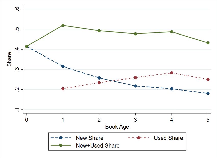
To further illustrate how the secondary market can affect outcomes, we conduct additional
counterfactual analyses varying the parameters of the model. First, we show that publishers
would benefit from the presence of the secondary market if (i) new and used books were less
substitutable and (ii) resale value was more important to students. These results have clear
implications for how firms can be expected to respond to secondary market competition. For
instance, as opposed to interfering with the secondary market, it may instead be optimal for
a firm to adjust its product characteristics in a way that reduces the substitutability of new
and used goods.
    Second, we explore the role of the mechanism determining used prices. During the period
of our data, university bookstores had extremely rigid pricing rules for used books, with used
books priced at essentially a constant fraction – 75 percent – of new books. This rigid used
book pricing stands in stark contrast to the much freer competition currently occurring on
Amazon.com and other online platforms. To analyze the impact of this competition on
market outcomes, we change the mechanism determining used prices to be a market clearing
mechanism and examine the model’s predictions. Consistent with data from Amazon and
other online platforms, we find that used prices lower than the rigid 75 percent rule at
university bookstores are needed to clear the market. The results also indicate that publisher
profits are lower with market clearing than under the rigid used book pricing mechanism,
which suggests that publisher incentives to interfere with the secondary market were likely
strengthened by the growth of firms like Amazon.7

1.1     Related Literature
The theoretical literature on the interaction between durable goods producers and secondary
markets is extensive, with the impact of secondary markets examined under a wide variety of
assumptions about consumer preference heterogeneity, the nature of product depreciation,
commitment, etc.8 The model we examine in this paper reflects one of the main trade-
offs described in Hendel and Lizzeri (1999) (and others): permitting resale increases buyer
willingness to pay and may facilitate the segmentation of new and used buyers, but also
introduces competition between new and used goods.
   7
     This implication is consistent with reports suggesting growing financial difficulties for textbook publish-
ers. Mitchell, J. (2014, August 27). A Tough Lesson for College Textbook Publishers. Wall Street Journal.
Church, S and Jinks, B. (2013, July 2). Cengage Learning Files for Chapter 11 Bankruptcy. Bloomberg.
   8
     Among others, relevant papers include Swan (1970); Miller (1974); Bulow (1982, 1986); Rust (1986);
Waldman (1993); Anderson and Ginsburgh (1994); Hendel and Lizzeri (1999); Oraiopoulos et al. (2012); and
Cui et al. (2014).

                                                       3
The empirical literature is considerably smaller but growing. In both Lazarev (2013)
(airline tickets) and Leslie and Sorensen (2014) (concert tickets), a key question when it
comes to the effects of secondary markets is the efficiency of the allocation of seats. Both
find that resale increases allocative efficiency, but that there are potentially offsetting effects
as well. For instance, Leslie and Sorensen (2014) find that resale induces costly rent-seeking
to obtain tickets in the primary market, which partially offsets the allocative efficiency gains
of resale. In the strategy literature, Bennett et al. (2015) hypothesize situations in which
firms will either benefit or be harmed by secondary markets – and thus how firms can be
expected to strategically respond – and then test those hypotheses using data from the US
concert ticket industry.
A major difference between our setting and those of Lazarev (2013), Leslie and Sorensen
(2014), and Bennett et al. (2015) is that tickets, unlike textbooks, are in some sense non-
durable. With tickets, there is a fixed time at which the good becomes worthless (the time
of the flight/event), whereas the time at which a textbook loses value – when the book is
revised – is a choice variable of the publisher. In addition, in contrast to tickets, textbooks
purchased on the primary and secondary markets are less likely to be perfectly substitutable.
The papers most closely related to our work are Shiller (2013) (video games) and Chen
et al. (2013) (automobiles), who also examine structural models to estimate the impact of
secondary markets. In their baseline specifications, both find that closing the secondary
market would substantially increase firm profits, by 50+ percent. These findings are similar
to our own results, which indicate that publisher profits would increase by 42.6 percent after
closing the secondary market.
Our contribution to this literature is four-fold. First, the models studied in this paper,
Shiller (2013), and Chen et al. (2013) are all tailored to the specifics of the industry under
examination. While such an approach facilitates more reliable measurement, the generaliz-
ability of the findings is less certain. The fact that all three papers indicate that firms would
profit from closing the secondary market suggests that, in real-world markets, the negative
effects of competition with used goods may tend to outweigh the benefits provided by resale
value. Second, our specific context allows us to straightforwardly model publishers’ strategic
revision choices, as opposed to assuming fully exogenous product depreciation. Third, we
explore the impact of the mechanism determining used prices, which affects both (i) resale
value and (ii) how strongly used goods compete for sales. Given the rise of internet com-
merce, the way in which used prices are determined in many markets may be meaningfully
different than in the past. Fourth, while structural estimation is prevalent in the economics
4literature, it is less so in the strategy literature (Grennan (2014) is a notable exception). We
view this paper as an example of the potential usefulness of structural methods in empirically
examining bedrock concepts in strategy like value creation and value capture.
The rest of the paper proceeds as follows. Section 2 describes the data and provides
descriptive statistics to motivate the structural model. Section 3 (demand) and section 4
(supply) develop the model and present the parameter estimates. Section 5 conducts the
counterfactual analyses. Section 6 concludes.
2 Data
Before proceeding to the full structural model, we begin by providing background on our
main data source, along with descriptive evidence about publisher and student behavior.
2.1 Textbook Sales Data
Our data covers economics textbook sales from about 1,800 university bookstores in the US
over the 11 year (22 semester) period from 1997 to 2007. The universities covered account
for around 60 percent of total college enrollment, and include everything from community
colleges to Ivy League universities. The data is currently produced by Nielsen and is the
same data used in Iizuka (2007) and Chevalier and Goolsbee (2009) (each with different
sub-samples of the full data, which covers additional subjects and years).
The data contains the aggregate (aggregating across universities) unit sales and total
revenue – both new and used – for each unique combination of International Standard
Book Number (ISBN)-year-semester, along with basic characteristics of the ISBN like the
title, author, and edition. The data also contains information about the ISBNs that are
assigned to students at the universities tracked, including a variable containing estimated
class enrollment. Several ISBNs correspond to the same “book” (combination of title and
author), both within and across semesters, so we manually combine these ISBNs on the basis
of the reported title and author. We then collapse the data to the book-year-semester level,
converting all monetary values to CPI-adjusted 2007 dollars. For example, a row in the
final dataset shows that in the fall semester of 2001, 17 percent of the estimated enrollment
for classes utilizing Greg Mankiw’s Principles of Macroeconomics bought a new copy of the
book at an average price of $115, while 28 percent of the estimated enrollment bought a
used copy at an average price of $84.
5Table 1: Final Sample Descriptive Statistics
Standard
Mean Median Deviation
New Sticker Price $124.11 $115.96 $18.47
Used Sticker Price $91.34 $85.36 $14.24
New Share 0.286 0.280 0.049
Used Share 0.238 0.238 0.040
Age at Revision 5.7 6.0 0.9
Enrollment 11,491 9,095 9,989
Page Length 631 576 165
Semesters 15.5 17 3.9
Editions 3.4 3.0 0.9
Notes: Prices are in CPI-adjusted 2007 dollars. Shares are calculated using the esti-
mated enrollment in classes utilizing the book as the market size. Book age is defined
as the number of semesters since the book was last revised.
The data covers more than 5,000 books in total, but sales are extremely concentrated.
The top 1 percent of books account for 52 percent of total new book revenue, while the bottom
90 percent of books account for only 11 percent of revenue. High-selling books are the focus
of the paper: low-selling textbooks, study guides, and books like Adam Smith’s The Wealth
of Nations are all excluded from the final sample. We also focus on introductory books, as
these books tend to be revised more frequently in a manner consistent with the structural
model. The enrollment data includes a description of the course, e.g. “Microeconomics:
Principles,” which we use to classify books as intro or non-intro according to whether the
majority of enrollment for the book is for an intro or non-intro course. The full list of 53
introductory books in the final sample and the precise sample restrictions we use are given
in section 7.1 in the appendix. Table 1 provides basic summary statistics about the books in
the final sample: the following subsections provide more detailed descriptive information.9
9
One limitation of the data is that it does not contain information about textbook sales beyond university
bookstores. To check for evidence of the growing importance of alternative sales channels (like Amazon.com)
over the period of the data, we have estimated models examining shares over time. If the data was increasingly
missing sales through other channels, shares would likely decrease markedly over time. A regression of (log)
combined new plus used share on semesters since the beginning of the data, (log) new sticker price, and
age fixed effects yields a (statistically insignificant) coefficient estimate that implies a roughly six percent
reduction in share over the 11 year period of the data. This result suggests that university bookstores still
sold the majority of volume for our sample even as companies like Amazon began to grow.
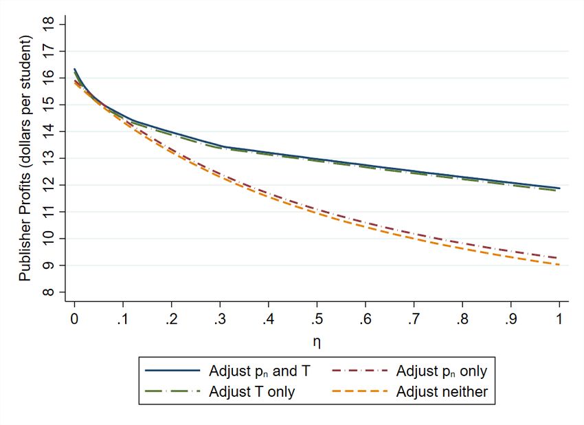
62.2 Price Patterns
There are several idiosyncracies in the market for textbooks during the period of our data
concerning pricing. First, both new and used sticker prices do not substantially vary over the
life of an edition. Second, used prices appear to be set at essentially a constant 75 percent
of new book prices. According to Chevalier and Goolsbee (2009), bookstore operators are
often constrained by contract with the university to price used books for no more than 75
percent of the new book price.10
To illustrate these characteristics of prices in our sample, Figure 1 plots (i) the average
new and used price for books in the final sample by book age (i.e., semesters since the last
revision) and (ii) the average ratio of the used price to the new price. As shown in the figure,
both new and used prices are essentially flat in book age. A test of the null hypothesis that
the averages are the same for each age yields a p-value of 0.95 for new prices and 0.89 for
used prices, thus failing to reject constant prices. The ratio of the used price to the new
price is also flat in book age, hovering just under 0.75. A regression of used price on new
price (without a constant) yields a coefficient estimate of 0.743 (and an R-squared of 0.998).
Figure 1: New and Used Prices by Book Age Newly revised books correspond to an age of
zero, at which point used books are not available. Age five combines all ages greater than or equal to five.
10
Bookstore operators are also often constrained to buy back current edition books for no less than 50
percent of the new book price, a fact which we utilize when modeling resale.
72.3 Revision Patterns
As shown above, sticker prices are more or less constant within an edition. However, effective
prices that take resale value into account vary. At the beginning of an edition when a
publisher is unlikely to revise the book, students who purchase the book can likely resell it
the following semester. If revision is imminent, on the other hand, there is a strong possibility
that the purchased book will become worthless for the purpose of resale in the subsequent
semester, since the bookstore has no use for old edition books that are no longer assigned.
Figure 2 plots the timing of revisions for books in the final sample. Books are essentially
never revised at early ages, whereas all books are revised within eight semesters (four years).
The most common revision timing is six semesters (three years). Chevalier and Goolsbee
(2009) study whether student purchasing behavior is responsive to impending revisions,
finding that “the data strongly support the hypothesis that students are forward-looking
with low short-run discount rates and that they behave as if they have rational expectations
of publishers’ revision behavior.” We rely on this finding in the structural model, in which
students correctly anticipate revisions and take expected resale prices into account when
making purchasing decisions.
Figure 2: Histogram of Revision Timing
82.4 Share Patterns
Figure 3 plots average shares – i.e., the percentage of estimated enrollment buying the new
or used copy of the book – by book age. When used books become available at age one, they
take 20 percent of the market. At the same time, the new book share falls by about half
that amount: 10 percentage points. This pattern suggests that some used book purchases
are driven by substitution from new to used, while other used book purchases are driven by
substitution from the outside good to used. Average used shares increase from age one to
age four, which may reflect increased availability of used books at university bookstores. The
combined new plus used share is relatively flat from age one to age four, but falls substantially
at age five. As most revisions occur at age six (Figure 1), this pattern is consistent with
students being forward-looking and sensitive to imminent revisions.11
Figure 3: New, Used, and Combined Shares by Book Age Newly revised books correspond
to an age of zero, at which point used books are not available. Age five combines all ages greater than or
equal to five.
11
The pattern is also potentially consistent with an increase in unobserved student-to-student transactions,
but unfortunately we do not have any data that speaks to this possibility.
93 Demand
We now develop a structural model of student purchase behavior. The focus of the model is
the competition between new books, their used versions, and the outside good. In addition
to non-purchase, the outside good also contains other options that we do not observe in the
data, like student-to-student transactions and piracy.
We assume that competition between textbooks of the same subject is weak, allowing us
to abstract away from professors’ textbook choice decisions. Competition between textbooks
might be weak due to professors largely making textbook decisions invariant of publishers’
pricing and revising policies, or if professors face large switching costs. In either case, the
effect of professor choice on the within-textbook competitive dynamics we model would
arguably be limited. More practically, adding an additional layer of decision making on
the demand side would substantially complicate the model and threaten the feasibility of
estimating it.
3.1 Model
After being assigned a textbook in semester t, students choose between the outside option
and buying the new or used version of the current edition of that book.12 The utilities of
student i in semester t from choosing new (n), used (u), or the outside good (∅) are:
uint = α0 − β · p̃int + ξnt + int
uiut = γ0 + γ1 · xt − β · p̃iut + ξut + iut (1)
ui∅t = 0 + i∅t .
xt is book age (i.e., semesters since last revision). We allow the utility of the used book
to change with age (according to γ1 ) in order to rationalize the observed pattern in the
data that used shares increase with age. A similar parameter for new books is not needed
to match the observed share patterns, so we exclude it for the sake of parsimony and to
clarify the identification of the model’s parameters.13 ξnt and ξut are demand shocks which
12
Purchases of an old edition, which the publisher no longer produces, are contained in the outside option.
13
By excluding such a parameter, we rule out quality deterioration as an explanation for declining new
sales as books age. We believe this restriction is largely reasonable for student demand. To the extent that
the primary use of a textbook is fulfilling class obligations, it is unclear why students would care about
the examples, etc. being a few years out-of-date. Up-to-date content may be more relevant for professors’
textbook choices, but again we abstract away from those choices in order to facilitate the computation of
the model.
10we assume to be mean zero and i.i.d. over time. Students’ idiosyncratic tastes are captured
by it ≡ (int , iut , i∅t ). For instance, a student who dislikes highlighted or underlined text
may have a small value of iut .
p̃ijt is the effective price of option j (new n or used u) that includes the utility (in
dollars) of resale and/or future use of the book. The effective price varies by student because
different students may assign different values to continued use of the book beyond the current
semester. Suppressing semester t for brevity from here on, the effective price p̃ij can be
decomposed as:
p̃ij = pj − δs · vi , (2)
where pj is the sticker price of the book, δs is students’ semester discount factor (assumed to
be constant across students), and vi is the value of the book to student i beyond the current
semester. The price of the new book pn is chosen by the publisher, while the price of the
used book pu is mechanically determined by:
pu = λ · pn . (3)
That is, the used price is a constant fraction of the new price. We adopt this mechanical
specification of used price formation given the institutional background and price patterns
outlined in section 2.2. That evidence indicates that λ ≈ 0.75, and hence we fix λ = 0.75
when estimating the model. (We examine the impact of changing the mechanism determining
used prices to be market clearing in section 5.2.)
The value of the book to student i beyond the current semester, vi , is the combination of
two potential sources of value: (i) resale and (ii) continued use of the book. If the publisher
revises the book – rendering the old edition worthless for the purpose of resale – students
receive the value from continued use of the book, ri . If the publisher does not revise the
book, students have the option either to keep the book and receive ri , or resell the book
and receive (1 − κ) · pu , where κ ∈ [0, 1] reflects the bookstore’s markup on used books.
During the period of our data, bookstores bought used books for 50 percent of the new price
and sold them for 75 percent of the new price (see section 2.2). Students therefore receive
50/75=2/3rds of the used price, and hence κ ≈ 1/3. We fix κ = 1/3 when estimating the
model.
Drawing on Chevalier and Goolsbee (2009), we assume that students correctly anticipate
when the publisher will revise the book. Denote the age at which revision will occur by T .
11vi can then be written as:
ri , x+1=T
vi = h i (4)
max (1 − κ) · pu , ri , x + 1 < T .
If the book will be revised next semester, the future value of the book to student i is the
value of continued use (ri ). If the book will not be revised next semester, on the other hand,
the future value of the book to student i is either the resale value ((1 − κ) · pu ) or the value
of continued use (ri ), whichever is greater.14 The max operator reflects student optimizing
behavior when faced with the choice between reselling the book and receiving (1 − κ) · pu
or keeping it and receiving ri . ri can therefore also be interpreted as student i’s reservation
value: the minimum resale value required for student i to be willing to resell.
Consider the impact of vi on student choice behavior. For example, if a student places a
high value on continued use of the book and does not discount the future much (i.e., δs · vi
is large), then the effective price of a book will be far below the sticker price, as the loss of
utility from paying the sticker price today is offset by the value of future use. Alternatively, if
students are myopic (δs = 0), then the effective price of a book is identical to the sticker price,
since myopic students assign no value to future options when making purchase decisions.
In the model, students differ from one another along two dimensions: (i) their idiosyn-
cratic tastes i ≡ (in , iu , i∅ ), and (ii) their reservation values ri . To facilitate computation
of the model, we assume that i and ri are independent.15 Given this assumption, the share
of students choosing option j (new n, used u, or the outside option ∅) is given by:
Z Z
1 j = argmax uik g (i )di gr (ri )dri ,
sj (x, pn ) = (5)
k∈C(x)
where the choice set C(x) is {n, ∅} if age x is equal to zero (in which case used books are
not available) and {n, u, ∅} otherwise. For notational convenience, we write shares sj (x, pn )
as depending only on age x and new price pn . 1[·] is an indicator function that takes a value
of one if the expression on the inside of the brackets is true – i.e., if option j delivers the
14
Given the evidence in section 2.2, we assume that the new price pn does not change within a book’s
edition. Therefore, students do not need to form an expectation over future prices in order to compute
equation (4), since absent revision the new and used price next semester will be the same as the current
semester.
15
Given independence and the assumption of logit tastes, the integration over i can be computed in closed
form. In addition, nothing in our data directly speaks to the correlation between i and ri , though in reality
at least some correlation may be present. For instance, students who assign a high value to continued use of
the book may also be more likely to have a strong preference for a new book.
12highest utility – and zero otherwise. g is the distribution of idiosyncratic tastes i and gr is
the distribution of reservation values ri .
We assume that tastes i are generalized extreme value distributed such that demand is
nested logit, with the new and used books nested according to nesting parameter ρ. ρ = 0
corresponds to simple logit demand – i.e., no correlation between in and iu – whereas ρ = 1
corresponds to perfect correlation. Nested logit demand allows for more flexible substitution
patterns than simple logit demand, which is important because the impact of the secondary
market on publisher profits may depend on the substitutability of new and used books. We
assume that reservation values ri are log-normally distributed with location parameter µr
and scale parameter σr .
3.2 Estimation
In this section, we outline the procedure we use to obtain estimates of the model’s parameters
and then report the results.
Parameters calibrated outside of the model
As discussed above, we fix λ = 0.75 and κ = 1/3 when estimating the model. We also fix the
parameters determining the distribution of student reservation values: µr and σr . Since our
textbook data does not include any information that directly pertains to reservation values
or resale decisions, we utilize an alternative source to inform these parameters. Specifically,
we utilize survey data collected from several thousand students at the University of North
Carolina between 2011 and 2013, as further documented in Spence (2015).16 As part of the
survey, students who purchased textbooks were asked: “Even if you plan on keeping your
book at the end of the semester, what is the lowest amount you would be willing to sell your
book for, once you are finished taking this course?” After scaling the survey responses to
be measured in CPI-adjusted 2007 dollars and restricting the data to books priced in the
range of our final sample, we estimate µr and σr by maximum likelihood using the reported
answers to this question. For students reporting $0, which is not in the support of a log-
normal distribution, we replace $0 with the minimum reported value above zero, which is one
cent. Measuring reservation values in tens of dollars, the resulting estimates are µ̂r = 1.178
and σ̂r = 1.085. Given these estimates, the median reservation value is about $32.50, with
85 percent of students valuing continued use of the book at less than $100. While we suspect
16
We thank Forrest Spence for providing us with this data.
13that heterogeneity across books in the distribution of reservation values may be present,
unfortunately we do not have sufficient data to link surveyed books to books in our sample,
and hence we assume that these parameters do not vary by book. To numerically integrate
over the distribution of reservation values, we use 1,000 random draws from the distribution.
It is also worth noting the difference between the time period of our textbook sales data
(1997 to 2007) and the survey data (2011 to 2013). It is possible that students’ reservation
values have meaningfully changed over time. For instance, recent students may have more
information about resale values than past students. While we assume that the survey re-
sponses accurately capture reservation values for our time period, we have also estimated
the counterfactuals with upward and downward adjustments to µ̂r and σ̂r . In the cases we
have examined, higher reservation values increase publisher profits, but do not appear to
affect whether closing the secondary market is profitable or not.
Remaining parameters
In contrast to many consumer products, we believe it is largely reasonable to assume that
the demand-side parameters in the textbook context do not vary substantially from product
to product (i.e., book to book). For many students, the primary use of a textbook is for
completing assignments, studying for tests, etc. In that case, the author or content of the
book may not have much bearing if any on student value. We therefore assume that the
remaining demand parameters θD ≡ (α0 , γ0 , γ1 , β, δs , ρ) are the same across the books in our
final sample.
To estimate the parameters with our aggregate data on textbook purchases, we follow
the method of moments estimation procedure developed by Berry et al. (1995). For each
candidate value of the demand parameters, we find the values of the demand shocks ξn and
ξu that equate the model-predicted and observed shares for each observation. Denote the
full vector of these values, which are functions of the demand parameters, by ξ(θD ). We
then estimate θD by exploiting assumed orthogonality conditions between ξ(θD ) and a set
of instruments. In particular, we solve:
min ξ(θD )0 ZW Z 0 ξ(θD ) , (6)
θD
where Z is a matrix of instruments and W is a positive definite weight matrix. For instru-
ments, we use indicator variables for each unique combination of book type (new or used)
and book age through age five, plus the page length of each book. This corresponds to
1412 instruments in total: six new book-age indicator variables (ages zero to five), five used
book-age indicator variables (ages one to five), and page length. Ages greater than five,
which account for less than 2 percent of observations, are grouped with the age five indicator
variable. For the weight matrix, we utilize W = (Z 0 Z)−1 , which is the efficient weight matrix
assuming homoskedastic errors (Nevo (2000b)).
Identification
The idea behind the book type-age indicator variable instruments is to allow detailed aspects
of the observed share patterns to inform the parameters. The base utility parameters α0
and γ0 strongly influence the overall level of new and used shares. γ1 , which controls the
evolution of the utility of used books over time, can be identified by how used shares change
with book age. The identification of the nesting parameter ρ and the student discount factor
δs is somewhat more nuanced. When used books become available at age one, ρ heavily
influences the extent to which the used book takes share from the new book vs. the outside
good. ρ can therefore be identified by the magnitude of the new plus used share increase once
used books become available, with the magnitude of the combined share increase decreasing
in ρ.17 δs can be identified by the responsiveness of demand to impending revisions. As a
benchmark, suppose that students are myopic (δs = 0), such that effective prices are identical
to sticker prices. In that case, shares will not respond to impending revisions. On the other
hand, if students are forward-looking with δs > 0, shares will fall in semesters in which the
book will be revised the following semester (at age five in particular).
A common concern when estimating demand models of this form is the possible endo-
geneity of prices: i.e., correlation between the demand shocks ξn and ξu and price pn . To
address this concern, we instrument for the price of each book with the page length of that
book. We collect the page length for the most recent edition of each book in the sample,
and therefore the instrument varies only across books. The length of a book affects the cost
of printing and shipping it, and therefore can be viewed as a marginal cost shifter. Indeed,
the correlation between new prices and page length is extremely strong: about 0.91. The
remaining requirement is that page length is uncorrelated with the demand shocks ξn and ξu .
The intuitive justification for this exogeneity assumption is that it is not clear why students
in an introductory economics class would have different underlying demand for the required
textbook if it was 800 pages compared to 600 pages (i.e., except for the effect via price).
17
The assumption that the non-price utility of the new book does not change with age is important for
this argument. Otherwise, a small new plus used share increase between age zero and age one might be able
to be explained by falling new book utility.
15This assumption would be violated if, for instance, longer textbooks contained more class
materials that students value. While we cannot rule out violations of this form, overall we
believe it is reasonable to assume that page length is exogenous to student preferences. We
also report the parameter estimates assuming that prices are exogeneous.
3.3 Results
The demand parameter estimates are reported in Table 2. The estimates assuming that
prices are exogenous correspond to specification (1), while the estimates instrumenting for
prices with book page length correspond to specification (2).
Table 2: Demand Parameter Estimates
Specification: (1) (2)
Instrument for price? No Page Length
Standard Standard
Description Parameter Estimate Error Estimate Error
Base new book utility α0 0.423 0.084 0.806 0.107
Base used book utility γ0 -0.120 0.094 -0.113 0.103
Used book age γ1 0.024 0.021 0.071 0.024
Price sensitivity β 0.164 0.011 0.247 0.018
Student discount factor δs 1 – 1 –
New/used nesting ρ 0.575 0.066 0.474 0.074
# of Books 53 53
# of Editions 180 180
# of Observations 824 824
Notes: The parameters governing used prices, resale prices, and the distribution of student reservation
values are fixed in estimation (λ = 0.75, κ = 1/3, µr = 1.178, and σr = 1.085). The student discount factor
converged to the upper bound of one in both specifications.
For both specifications, the student discount factor converged to the upper bound of one.
While consistent with Chevalier and Goolsbee (2009), who also estimate student discount
factors statistically indistinguishable from one, it is perhaps surprising that college students
would exhibit such forward-looking behavior. An interesting theory we have heard that can
potentially help explain this result is that money for the initial textbook purchase may often
be supplied by parents, whereas the proceeds from resale may be retained by students. In
that case, student purchase behavior will be particularly sensitive to resale value.
To facilitate interpretation of the remaining parameters, we calculate the implied (i)
shares and (ii) own and cross-price elasticities for a book with pn = $124.11 and T = 6
16Table 3: Estimated Shares and Elasticities
Panel A: Shares
Book Age New Used New+Used
0 0.410 – 0.410
1 0.259 0.222 0.480
2 0.246 0.242 0.488
3 0.233 0.263 0.496
4 0.221 0.284 0.505
5 0.151 0.223 0.374
Panel B: Elasticities
New Used Outside
New -3.71 1.75 –
Used 2.07 -2.60 –
Outside 0.58 0.49 –
Notes: All statistics are calculated for a book with pn = $124.11, T = 6, and
demand parameters equal to the point estimates for specification (2) in Table
2. The parameters governing used prices, resale prices, and the distribution of
student reservation values are fixed at the values utilized in estimation. The
elasticities are averages between age one and age five. The columns are price
changes and the rows are quantity changes: e.g., a 1 percent increase in the price
of the new book is estimated to yield a 3.71 percent decrease in the new book
share and a 2.07 percent increase in the used book share.
(the mean values for books in the final sample, rounding T to the nearest integer) and
demand parameters equal to the point estimates for specification (2). We prefer specification
(2) because of the larger estimated price sensitivity, which is consistent with the possible
endogeneity of prices. For the elasticity calculations, we sever the mechanical link between
new prices and used prices (equation (3)) to isolate demand-side behavior. The results are
reported in Table 3.
The estimated share patterns exhibit the same noteworthy characteristics that appear
in the aggregate share data depicted in Figure 3. The new plus used share jumps up when
used books become available at age one. The used share then continues to climb while the
new plus used share remains relatively constant. At age five – the semester before revision
– shares fall sharply due to the increase in effective prices.
The estimated cross-price elasticities indicate that substitution between new and used
books is much stronger than substitution toward the outside good. Estimated diversion ratios
(not reported in the table) are also illustrative of this point. Of the students substituting
17away from the new book following a price increase, we estimate that 63 percent of them
would switch to buying used. Proportional substitution based on shares implies a much
lower diversion ratio of 32 percent. It is also worth noting that the true price elasticity faced
by publishers is weaker than the -3.71 presented in Table 3. When a publisher increases
the price of the new book, used prices increase mechanically in turn, which dampens the
substitution to used books. The new book own price elasticity taking this linkage into
account is estimated to be -1.54.
4 Supply
The purpose of explicitly modeling student purchase behavior is so that we can forecast
how demand would change in response to a shift in the environment, such as closing the
secondary market (i.e., banning resale). Besides the demand response, whether publishers
would benefit from closing the secondary market depends on their cost structures, and also
their own strategic responses to the change in environment. We therefore also implement a
structural model of publisher pricing and revising decisions, and combine that model with
observed publisher behavior to estimate publisher costs.
4.1 Model
We assume that each publisher has two choice variables: (i) the price of the new book pn
and (ii) the length of the revision cycle T . The publisher commits to both of these decisions:
the price cannot be changed, nor can the revision cycle be adjusted. These assumptions are
consistent with the known institutional details of the industry. As shown in section 2.2, new
book prices are essentially flat within edition. Moreover, publishers often sign contracts with
textbook authors that specify the timing of revisions (Chevalier and Goolsbee (2009)).
Each semester, the publisher earns the flow profits from sales of the book. In semesters
where the book is revised, the publisher also incurs a fixed revising cost. We assume that
publishers evaluate price and revision cycle choices by the average per-semester profits gen-
erated by those choices. Normalizing the number of students assigned the book to one, the
publisher’s optimization problem is thus:
−1
TP
sn (x, pn ) · (pn − c)
x=0 F
max − , (7)
pn ,T T T
18where T is constrained to be an integer greater than or equal to one.18 c is the marginal cost
of the book and F is the fixed revising cost (normalized by the number of students). The
first term in the maximand reflects profits from book sales, while the second term reflects
revision spending. Shortening the revision cycle implies less frequent competition with used
books, but also higher revision spending. For instance, if T = 1, the publisher will never
face competition from used books, but the publisher will also incur the revising cost F every
semester. The optimal revision cycle balances these effects.
4.2 Estimation
The parameters to be estimated on the supply side of the model are the marginal cost c
and fixed revising cost F for each book. These parameters may vary across books due
to differences in book length, fees paid to authors, etc. We estimate these parameters for
the most recent edition of each book for which we observe the revision timing by finding
the values of c and F such that the solution to the publisher’s optimization problem (7)
is equal to the observed new book price and revision timing. This procedure is analogous
to the recovery of marginal costs in the static case (e.g., Nevo (2000a); Nevo (2001)), with
the addition of the revising decision and associated fixed revising cost. When solving the
publisher’s optimization problem for each book, we set the demand parameters equal to the
point estimates for specification (2) in Table 2.
The identification of the supply parameters is relatively straightforward. Intuitively, the
optimal revision age is increasing in the fixed revising cost, so the F for each book can be
identified by the age at which the book is revised. Similarly, the optimal price is increasing
in marginal cost, so the c for each book can be identified by the price of the book. Since
revision timing is integer-valued, this procedure yields an interval of fixed revising costs such
that the model-predicted revision timing is equal to the observed revision timing. Marginal
costs are point-identified.
4.3 Results
The supply parameter estimates are reported in Table 4. Mean estimated marginal costs are
$38.78, or about 5.7 cents per page. A report by the educational product firm Follett esti-
18
To simplify the computation of optimal publisher behavior, we compute shares deterministically by
setting the demand shocks ξn and ξu equal to zero. Without this simplification, solving the publisher’s
optimization problem requires (i) specifying the distribution of the demand shocks and (ii) integrating over
the demand shocks for all semesters prior to revision, which is an integral over 2T − 1 dimensions.
19Table 4: Supply Parameter Estimates
Standard
Parameter Mean Median Deviation
Marginal cost c $38.78 $31.55 $26.06
Marginal cost c per page $0.057 $0.056 $0.028
Fixed revising cost F lower bound $20.24 $18.50 $6.47
Fixed revising cost F upper bound $26.45 $24.64 $8.33
Fixed revising cost F midpoint $23.35 $21.57 $7.40
Notes: All values are in CPI-adjusted 2007 dollars. The fixed cost estimates are normalized by
student enrollment.
mates that $33.60 of a $100 textbook’s price goes to printing and shipping.19 The estimated
marginal costs therefore appear to be similar to industry sources.
Turning to the estimated fixed revising costs, recall that the estimates are normalized
by student enrollment. Books in the final sample have an average estimated enrollment
of 11,491 (Table 1). The data captures roughly 60 percent of total college enrollment, so
scaling enrollment up to the universities not included in the data yields a total enrollment
estimate of 11,491/0.6=19,152. Multiplying the mean estimated fixed revising cost mid-
point by this estimate of enrollment generates revision costs of $23.55*19,152≈$450,000. A
report by the Association of American Publishers suggests that these numbers are in the
ballpark of – though somewhat less than – industry claims: “Developing a new textbook
and accompanying learning tools can cost more than $1 million.”20
5 Counterfactual Analysis
In this section, we use the estimated structural model to simulate student and publisher
behavior in alternative market environments. In section 5.1, we close the secondary market
by banning resale. When the secondary market is closed, students can still buy new books
but used books cannot be bought or sold. For publishers, closing the secondary market
eliminates competition with used books, but also eliminates their ability to charge for resale
value. Which force dominates, and on what parameters does the answer hinge?
In section 5.2, we convert the mechanism determining used prices to be market clearing.
19
Follett Insight. The Real Cost of Textbooks – and Affordable Options for Students.
20
Association of American Publishers, Inc. Why PIRG is Wrong: Myths and Facts About College Text-
books, 2006.
20The main purpose of this exercise is to understand how publisher incentives to close the
secondary market might have been affected by the rise of non-university bookstore inter-
mediaries like Amazon.com, where sellers are not held to rigid pricing rules. Are publisher
incentives to close the secondary market strengthened or weakened when used prices are
determined by market clearing?
We calculate all estimates for a book with demand parameters equal to the point estimates
for specification (2) in Table 2 and supply parameters equal to the means in Table 4. The
parameters governing used prices, resale prices, and the distribution of student reservation
values are fixed at the values utilized in estimation.21
5.1 Closing the Secondary Market
When the secondary market is closed, students no longer need to anticipate revisions: with
no resale, the effective price of new books is always the sticker price less the student’s
discounted reservation value (i.e., pn − δs · ri ). Closing the secondary market also eliminates
the publisher’s incentive to revise the book, as revision no longer has an impact on student
demand. The publisher instead faces a standard static pricing problem, choosing price to
maximize flow profits.
Table 5 reports estimates of the effect of closing the secondary market on a variety of
market outcomes. A first thought is that closing the secondary market would allow the
publisher to charge a higher price, because competition with used books disappears. In fact,
however, the opposite occurs, with the new sticker price falling by 6.9 percent. When the
secondary market is closed, the publisher can no longer charge students for resale value,
which puts downward pressure on the new price. The new effective price, on the other
hand, rises considerably. Without resale, many students face much higher effective prices
because they are no longer able to recoup some of the purchase price via resale. 31.2 percent
of students purchase the new book when the secondary market is closed, which is larger
than the average new share when the secondary market is open (24.0 percent). At age zero,
however, the new share is higher when the secondary market is open, because at that point
there is no competition with used books and students can benefit from resale in the next
semester (which increases student to willingness to pay). The benefit of closing the secondary
market comes at non-zero ages where competition with used books is particularly damaging.
21
The exact values of the parameters are as follows. Demand: α0 = 0.806, γ0 = −0.113, γ1 = 0.071,
β = 0.247, δs = 1, ρ = 0.474. Supply: c = $38.78 and F = $23.35. Other parameters: λ = 0.75, κ = 1/3,
µr = 1.178, and σr = 1.085. The demand shocks ξn and ξu are set to zero to facilitate the computation (see
footnote 18).
21Table 5: Closing the Secondary Market
Open Closed Percent
(Status Quo) (No Resale) Change
New Sticker Price $129.03 $120.07 -6.9%
New Effective Price $46.21 $61.10 32.2%
New Share 0.240 0.312 29.9%
Age=0 0.395 0.312 -21.0%
Age>0 0.209 0.312 49.1%
Used Sticker Price $96.77 – –
Used Effective Price $14.91 – –
Used Share 0.246 – –
Age at Revision 6 – –
Publisher Profits $17.77 $25.34 42.6%
Flow Profits $21.66 $25.34 17.0%
Revision Spending $3.89 $0.00 -100.0%
Student Surplus $36.39 $28.26 -22.4%
Bookstore Profits $6.61 $0.00 -100.0%
Total Surplus $60.77 $53.60 -11.8%
Notes: The estimates are calculated for a book with demand parameters equal to the point
estimates for specification (2) in Table 2 and supply parameters equal to the means in Table 4.
The parameters governing used prices, resale prices, and the distribution of student reservation
values are fixed at the values utilized in estimation. See footnote 21 for the exact parameter
values. All monetary values are in CPI-adjusted 2007 dollars. All statistics are averages
across the distribution of student reservation values and book ages. Bookstore profits capture
the markup on used books, assuming no other revenues or costs of operation. Publisher profit,
student surplus, and bookstore profit estimates are per student. Total surplus is the sum of
publisher profits, student surplus, and bookstore profits.
Overall, we estimate that publisher profits increase by 42.6 percent when the secondary
market is closed. This result indicates that the detrimental effect from used book com-
petition on publisher profits far exceeds any benefits that are generated by resale value.
As discussed above, new sticker prices actually fall when the secondary market is closed.
Rather than greater pricing power, the large increase in profits instead comes from (i) a
higher quantity sold and (ii) less revision spending. The decrease in revision spending ac-
counts for $3.89/($25.34-$17.77)=51 percent of the increase in profits, with the increase in
flow profits accounting for the remaining 49 percent.
The complete absence of revision spending when the secondary market is closed is ar-
guably a somewhat extreme case. However, even if the publisher is held to revising every six
semesters – as in the status quo case – we estimate that publisher profits would be $25.34-
22$3.89=$21.45, which is still 20.7 percent higher than publisher profits when the secondary
market is open. In short, given the estimated parameter values, the results strongly suggest
that publishers would benefit from closing the secondary market.
The rise of E-Textbooks, where digital rights management technology can more readily
prevent resale, is consistent with the result that publishers would profit from closing the
secondary market. In addition, even if publishers cannot directly close the secondary market,
they can take actions that make resale less prevalent. For instance, publishers now often
rent textbooks to students, which allows publishers to make sales that do not subsequently
compete with new books in future semesters.22,23
It is also worth highlighting that total surplus falls by 11.8 percent when the secondary
market is closed: the increase in publisher profits from closing the secondary market is less
than the combined decrease in student surplus and bookstore profits. This result echoes the
intuition from value-based strategy provided at the outset of the paper. While a smoothly
functioning secondary market may create value, it is also capable of impeding firm value
capture to an extent that the firm would prefer the secondary market to be closed entirely.
Can publishers benefit from the secondary market?
While the results suggest that closing the secondary market would increase publisher profits
at the estimated parameter values, for other parameter values the presence of the secondary
market is beneficial to publishers. Recall the two main forces through which the secondary
market affects publisher profits: competition between new and used books harms publishers,
while resale value benefits publishers. By varying model parameters that capture these two
forces, we can examine the subsequent quantitative impact on the profitability of closing the
secondary market.
To examine the impact of competition between new and used books, we vary the nesting
parameter ρ, which governs the correlation in students’ idiosyncratic tastes for new and
used books. For high values of this parameter, tastes are highly correlated, whereas for low
values new and used books are less substitutable. To examine the impact of resale value, we
introduce an additional parameter, radj , that scales the estimated student reservation values
ri . In particular, we let ri0 = radj · ri for all i and then solve the model for the adjusted
22
Lewin, T. (2009, August 13). Textbook Publisher to Rent to College Students. New York Times. Besides
rental, customized textbooks containing additional professor-specific materials may also be more difficult for
students to resell.
23
In section 7.2 in the appendix, we examine an additional counterfactual in which we permit publishers
to rent books in addition to selling them. We find that publishers benefit from having a rental option, as it
allows publishers to attract students with low reservation values without decreasing the price of new books.
23You can also read