Housing markets and migration - Evidence from New Zealand - Motu Working Paper 19-14 Motu Economic and Public Policy Research - MBIE

Housing markets
and migration –
Evidence from New
Zealand

Dean R. Hyslop, Trinh Le, David C.
Maré and Steven Stillman
Motu Working Paper 19-14
Motu Economic and Public Policy
Research
July 2019

Housing markets and migration – Evidence from New Zealand

Document information
Author contact details
Dean R. Hyslop
Senior Fellow, Motu Economic and Public Policy Research Trust
dean.hyslop@motu.org.nz

Trinh Le
Fellow, Motu Economic and Public Policy Research Trust
trinh.le@motu.org.nz

David C. Maré
Senior Fellow, Motu Economic and Public Policy Research Trust
dave.mare@motu.org.nz

Steven Stillman
Professor, Department of Economics and Management, Free University of Bozen-Bolzano, Italy
steven.stillman@unibz.it

Acknowledgements
Funding for this study was provided the Ministry of Business, Innovation & Employment. We
thank Andrew Coleman, Matthew Curtis, Anne-Marie Masgoret, Jacques Poot and Manuila Tausi
for valuable discussions and comments.

Disclaimer
The results in this paper are not official statistics, they have been created for research purposes
managed by Statistics New Zealand. The opinions, findings, recommendations and conclusions
expressed in this paper are those of the authors not Statistics New Zealand, the Ministry of
Business, Innovation & Employment, or Motu Economic & Public Policy Research. Access to the
data used in this study was provided by Statistics New Zealand under conditions designed to
give effect to the security and confidentiality provisions of the Statistics Act 1975. The results
presented in this study are the work of the authors, not Statistics NZ.

 ii

Housing markets and migration – Evidence from New Zealand

Abstract
This paper analyses the relationship between local area housing and population size and
migrant-status composition, using population data from the 1986–2013 New Zealand Censuses,
house sales price data from Quotable Value New Zealand, rent data from the Ministry of
Business, Innovation and Employment, and building consents data from Statistics New Zealand.
Measured at the Territorial Local Authority and Auckland Ward (TAW) area level, we estimate
the elasticity of house prices with respect to population is 0.4-0.65, similar but smaller elasticity
of apartment prices, but find no evidence of any local population effects on rents. We also
estimate the elasticity of housing quantity with respect to population of about 0.9. Although
international migration flows are an important contributor to population fluctuations, we find
little evidence of systematic effects of international or domestic migrant composition of the local
population on prices or quantity. In particular, despite there being a strong correlation between
immigration and house price changes nationally, there is no evidence that local house or
apartment prices are positively related to the share of new immigrants in an area. Repeating the
analysis for more narrowly defined areas within Auckland, we estimate a smaller house price
elasticity with respect to population in the range 0–0.15. Finally, our analysis suggests that
longer-term housing supply is relatively elastic, and demand inelastic, with respect to price.

JEL codes
J61, R23

Keywords
Immigration, population, housing markets, house prices, rents

Summary haiku
People need houses.
More people higher prices,
wherever they’re from.

Motu Economic and Public Policy Research
PO Box 24390 info@motu.org.nz +64 4 9394250
Wellington www.motu.org.nz
New Zealand

© 2019 Motu Economic and Public Policy Research Trust and the authors. Short extracts, not exceeding
two paragraphs, may be quoted provided clear attribution is given. Motu Working Papers are research
materials circulated by their authors for purposes of information and discussion. They have not
necessarily undergone formal peer review or editorial treatment. ISSN 1176-2667 (Print), ISSN 1177-
9047 (Online).

 iii

Housing markets and migration – Evidence from New Zealand

Table of Contents
1 Introduction 1

2 Background and literature review 4

3 Data and descriptive analysis 5
 3.1 Population data 5
 3.2 Housing market data 7
 3.3 Descriptive statistics 8
 3.4 Exploratory analysis of house prices and population 10

4 Model framework 12

5 Analysis and results 15
 5.1 Residential house prices 15
 5.2 Alternative housing price outcomes 18
 5.3 Alternative area-level observations 20
 5.4 Miscellaneous analyses 21

6 Concluding discussion 21

References 23

Recent Motu Working Papers 39

Table of Figures
Figure 1: New Zealand net migration and house price changes, 1963–2016 25
Figure 2: New Zealand house price versus population changes, Census 1986–2013 25
Figure 3: Inter-censal house price versus population changes, Census 1986–2013 26

Table 1: Sample characteristics, 1986–2013 Census years 27
Table 2: Sample characteristics, by sub-population 28
Table 3: Exploratory log(House price) regressions, 1986–2013 Census years 29
Table 4: Regressions of log(House prices), 1991–2013, TAW 30
Table 5: Regressions of log(House prices) changes, 1991–2013, TAW 31
Table 6: Regressions of Other outcomes, 1991–2013, TAW 32
Table 7: Regressions of Other outcome changes, 1991–2013, TAW 33
Table 8: Housing Demand and Supply elasticities, 1991–2013, TAW 34
Table 9: Auckland house price regressions, 1991–2013, Area Units 35
Table 10: Outcome changes regressions, 1991–2013, TAW – Asymmetric effects 36

 iv

Housing markets and migration – Evidence from New Zealand

1 Introduction
There has been widespread recent concern that strong increases in immigration flows have
caused a housing crisis in New Zealand.1 In fact, aggregate time series analyses by Coleman and
Landon-Lane (2007) and McDonald (2013) estimate that a one percent increase in population
from immigration is associated with an increase in house prices on the order of 10 percent. In
this paper, we examine the aggregate and local area relationships between population changes
and house price growth over the census-based period from 1986 to 2013: although this period
does not capture the substantial changes that have occurred since 2013, it does cover earlier
periods of similarly strong increase. Between 1986 and 2013, the population of New Zealand
increased by 37%, from 3.2m to 4.4m. Although the majority of this increase was due to natural
increase (80%), migration flows did change the composition of the NZ population as well as the
size. The number of foreign-born New Zealanders more than doubled (108%), whereas the New
Zealand-born population rose by only 8%. Over the same period, the average real (inflation-
adjusted) house price increased by about 140%.
 There are several issues with aggregate time series analyses of the effects of immigration
on house prices.2 Both immigration and house prices are pro-cyclical over the business cycle,
and also tend to co-vary with other asset prices, so attributing cause and effect from correlated
movements is difficult. Previous NZ research has found far more muted local and regional house
price responses to population shocks (Maré, Grimes, and Morten 2009; Stillman and Maré
2008).3 This may be because while an immigration-driven population shock into an area will
increase the demand for local housing, it may also affect the location decisions of the native
population.4 In addition, immigrants can affect housing supply through factors such as housing
investment and expertise in the building industry.

1 See, for example, Economist: Cut migrant numbers to bring down Auckland house prices
(https://www.nzherald.co.nz/business/news/article.cfm?c_id=3&objectid=11651226), Reserve bank: Migration key
to housing crisis (https://www.nzherald.co.nz/nz/news/article.cfm?c_id=1&objectid=11670498), Immigration peak
to fuel house prices (https://www.nzherald.co.nz/nz/news/article.cfm?c_id=1&objectid=11453363). Auckland's
population grew by 62%. However, the number of NZ-born grew by 20%, whereas the number of foreign-born grew
by 160%. It is probably the increased presence of foreign born, rather than immigration flows, that lead people to
think that immigration is causing house price increases.
2 See Fry (2014) for a recent review of the broader macroeconomic effects of migration in New Zealand. Cochrane and

Poot (2016) provide a recent review of the New Zealand literature on the impact of international migration on house
prices; and Cochrane and Poot (2020) provide an international review of the local housing market effects of
immigration.
3 For example, Stillman and Maré (2008) estimate the local housing price elasticity with respect to area population is

in the range of 0.2–0.5. They find no evidence that local house prices are positively related to the inflow of foreign-
born immigrants to an area, but that there is a strong positive relationship between inflows of New Zealanders
previously living abroad into an area and the appreciation of local housing prices, with a one percent increase in
population due to returning New Zealanders associated with a 6-9 percent increase in house prices.
4 For example, Saiz and Wachter (2011) and Sá (2014) find significant local area out-migration of the native

population following increases in immigration, which affects the spatial demand for housing by natives.
 1

Housing markets and migration – Evidence from New Zealand

 We focus on how local area population change, both in terms of its size and composition,
affects the price and supply of housing in those areas. To do this, we outline a simple demand
and supply model for local housing, from which we derive reduced form equations for both the
price and quantity of housing. Our primary focus is the price of housing, as measured by average
house prices in an area, but we also consider average apartment prices as well as average rents
and also quantity measures of housing supply.
 Our analysis builds on Stillman and Maré (2008), and we extend their analysis in several
ways. First, we extend the period of analysis to include data from the 2013 census. Second, we
include information on building consents to proxy for local area housing supply conditions.
Finally, we consider the responsiveness of housing supply over the period. Our main focus is on
the local area level relationship between the price of housing, as measured by housing prices
and rents, and population, with emphasis on whether the relationship depends on the migrant-
status composition of the population. To do this, we define various sub-populations by whether
or not they are New Zealand born, and their recent (inter-censal) international and domestic
migration status, and analyse the relationship between house prices and the share of the local
population in each group.
 We first provide a connection to the aggregate time series literature, with an exploratory
analysis of the relationship between local-area house sale prices and local-area and aggregate
(NZ) population.5 The results of simple regressions show that aggregate population has a more
dominant effect on local house prices than local-area population: in a house-price change
regression, we estimate an elasticity of house prices with respect to aggregate population of 9.9,
which is in the range of long-run elasticities estimated by Coleman and Landon-Lane (2007),
while the elasticity with respect to local population is about 0.4.6 Our subsequent analysis
abstracts from the possible confounding effects of macroeconomic factors, and focuses on the
relationship between housing and population measured at the local area.
 We then provide a more detailed analysis of the relationship between local area housing
prices and rents, and population size and composition. We outline a conceptual demand and
supply framework for the local-area housing market, which motivates a reduced-form equation
approach to estimating the relationship between the price (and quantity) of housing and
population characteristics. Recognising that there may be significant segmentation of the
housing market between owning and renting, and also possibly between houses and apartments,
we consider four alternative ‘price’ specifications: house sale prices, apartment sale prices,
house rents, and apartment rents. Considering these different measures is also important

5 Our primary analysis is based on Statistics New Zealand’s 78 territorial authorities and Auckland wards (TAW),
which consist of 66 territorial local authorities (TLA), with the Auckland TLA disaggregated into 13 wards. We also
repeat our main analyses using 140 labour market areas (LMA).
6 Although the estimates are similar in our preferred regression specifications that control for the local-area

population composition and other factors, the magnitude and statistical significance of the estimated aggregate
population effects depend on the particular specification adopted, and can be statistically insignificant, substantially
smaller, and even negative.
 2

Housing markets and migration – Evidence from New Zealand

because house and apartment prices are likely to reflect both the consumption value of housing
and asset price effects, while rents should be dominated by the value of housing services. In
addition, we estimate regressions for two measures of housing ‘quantity’: the number of
occupied dwellings, and the number of bedrooms. For each of these outcomes, we estimate both
(log(price) or log(quantity)) ‘levels’ and ‘changes’ regression specifications.
 In our primary analysis of house sale prices at the TAW area level, we find consistently
positive population size effects on house prices. The estimated local area price elasticities with
respect to population range from 0.4 in our preferred ‘levels’ specification to 0.65 in our
preferred ‘growth’ specification, meaning that a ten percent increase in local area population is
associated with a 4–6.5 percent higher house prices. However, conditional on the population
size, we find little evidence that the composition of the local-area population systematically
affects house prices, after controlling for observable differences in the socio-demographic
characteristics of areas. In particular, the only consistent result is that, relative to the share of
staying New Zealanders in an area, a higher share of moving New Zealanders is associated with
higher house prices. We find no evidence that a higher share of new immigrants is associated
with higher house prices. Our analysis of apartment prices provides qualitatively similar,
although weaker and less precisely estimated, population results. The results from LMA level
analysis are qualitatively similar, but with relatively stronger population effects on apartment
prices than house prices.
 In contrast to the analysis of prices, we find consistently small and statistically
insignificant population size effects on both house and apartment rents. However, we do find
significant population composition effects on rents, with the relative shares of all ‘moving’
subgroups positively affecting local area rents – i.e. relative to those who are New Zealander
born and don’t move area, all other population groups positively affect rents. The absence of any
population size effects on rents provides suggestive evidence of the importance of asset price
factors underlying the population effects on house and apartment prices.
 Our analysis of housing quantity finds strong population effects on both the number of
dwellings and the number of bedrooms, with elasticities of close to 0.9 for both quantity
measures. We also find that the share of returning New Zealanders in an area is most positively
associated with each quantity measure. Combined with the house prices estimates, these results
suggest that longer-term housing supply is relatively elastic with respect to price (1.2), and
housing demand is inelastic (-0.3).
 Finally, given the importance of Auckland as an immigrant destination and the strength of
recent and past housing markets there, we reanalyse the population effects on house prices in
Auckland using more narrowly defined area unit (AU) data. The results from this analysis find
smaller house price elasticities with respect to population (0–0.15), and are robust to allowing
for neighbouring area spillover effects. Together with broader area analyses, these results are

 3

Housing markets and migration – Evidence from New Zealand

consistent with the hypothesis that the smaller the area of focus the smaller will be the impact of
population on housing.
 The rest of the paper is organised as follows. The next section provides some background
context for the research. In section 3 we discuss the data collated from various sources that are
used in the analysis, describe summary statistics and patterns, and present the exploratory
analysis of the relationship between house prices and population. Section 4 outlines a
conceptual model of the housing market; we present and discuss the analysis and results in
section 5; and the paper concludes with a discussion in section 6.

2 Background and literature review
A strong associative relationship between New Zealand’s real (inflation-adjusted) house price
changes and net international migration flows is apparent and motivates ongoing public and
policy concern about the effect that immigration has on housing affordability. However, given
the cyclical nature of both immigration and house price growth, disentangling confounding
common cyclical factors to identify the causal effect of immigration on house prices is potentially
difficult. For example, Figure 1 describes the historical relationship, which highlights two
features. First, there is a strong co-movement between the two series: the correlation coefficient
between the series is 0.56. Second, the annual house price percentage increases are an order of
magnitude greater than the net migration as a percentage of the population: the estimated
coefficient in a simple regression of house price changes on net migration is 8.7. We suspect
these two features largely underpin Coleman and Landon-Lane’s (2007) and McDonald’s (2013)
macro estimates that a 1 percent population increase from migration is associated with about a
10 percent increase in house prices nationally.
 In contrast to these large macro-estimated elasticities of the relationship between national
population and house price growth, micro-focused analyses of the relationship between local
area house prices to population find much smaller elasticities. Cochrane and Poot (2020)
reviews the international literature, together with a case study focus on New Zealand. We briefly
highlight some of the main findings here. In fact, the recent international literature finds mixed
evidence on the impact of immigration on house prices at the local area. For example, in the US,
Saiz (2003) estimated a housing rent elasticity of about 1 in Miami following the large increase
in the immigrant population associated with the Mariel boatlift in 1980. Saiz (2007) also
estimated similar magnitude rent and house price elasticities associated with immigration
driven population growth in major immigrant destination cities. In Switzerland, Degen and
Fischer (2017) estimate the elasticity of house prices with respect to population growth from
immigration was close to 3. In contrast, Akbari and Aydede (2012) estimate trivially small house
price elasticities in Canada, and Sá (2014) finds that immigration has a negative effect on house

 4

Housing markets and migration – Evidence from New Zealand

prices in UK.7 Sá attributes the negative effect to an outward mobility response of the native
population following immigrant inflows; strong spatial sorting effects following immigration
shocks have also been found by Saiz and Wachter (2011).
 The only previous New Zealand study to examine the local impacts of population on house
prices is by Stillman and Maré (2008). Using census level population data linked to house prices
and rents over the period from 1991–2006, Stillman and Maré (2008) estimate relatively small
local area house prices elasticities with respect to population on the order of 0.2–0.5, and rent
elasticities that are generally zero or negative. More detailed analysis of the relationship by the
population components finds no evidence that stronger growth of recent immigrants to an area
positively affects house prices; however, they do find that a higher rate of recently returned New
Zealanders from abroad strongly affects house prices, and also generally positively affects rents
(although with weak statistical significance).

3 Data and descriptive analysis
The analysis presented in this paper uses data assembled from several sources. First, we use
population and dwelling data from New Zealand Censuses of Population and Dwellings between
1986 and 2013;8 second, we use data from Quotable Value New Zealand (QVNZ) to derive
average house sales prices; third, we use data from the Ministry of Business, Innovation &
Employment’s (MBIE) Tenancy Bonds database to derive average rents; and finally, we derive
information on new houses and apartments, as well as alterations and extensions, from building
consents data provided by Statistics New Zealand. In this section, we discuss the main
characteristics of each of these data sources.

3.1 Population data
This paper uses unit-record data for the usually resident population from the 1986, 1991, 1996,
2001, 2006 and 2013 Censuses to identify the population and characteristics of different local
areas in New Zealand. The Census collects information on each individual’s country of birth,
their current usual residential location and their usual residential location (including overseas)
five years before the census date. We use this information to classify individuals as being ‘new
immigrants’, ‘returning New Zealanders’, ‘previous immigrants’, or ‘local New Zealanders’ where
‘new immigrants’ are individuals not born in New Zealand who resided outside the country 5
years previously, ‘returning New Zealanders’ are individuals born in New Zealand who resided

7 However, Aitken (2014) estimates modest positive effects of immigration on local area rents in the UK, with an
elasticity of about 0.15.
8 See the disclaimer on page ii.

 5

Housing markets and migration – Evidence from New Zealand

outside the country 5 years previously and the remaining two categories consist of non-NZ born
and NZ born individuals, respectively, who resided in New Zealand 5 years previously.9
 Each individual’s current usual residence is coded to a census meshblock, which is the
smallest geographic area used by Statistics New Zealand in the collection and processing of data
and is typically aligned to cadastral boundaries. Meshblock boundaries vary across censuses and
we allocate each year's meshblocks to a consistent set of more aggregated geographic areas. In
the current paper, we consider two definitions of housing markets, namely 78 territorial local
authorities and Auckland wards (TAW) and 140 labour market areas (LMA).10 The TAWs are
based on 66 territorial local authorities (TLA) but with the Auckland disaggregated into 13
wards.11 This definition is similar to the 73 TLAs studied by Stillman and Maré (2008). The LMAs
used in our analysis are identical to the 140 LMAs examined by Stillman and Maré (2008), which
were derived by Newell and Papps (2001).12
 The population base for our analysis of housing demand is the usually resident population
aged 18 and over in each geographic area, excluding individuals for whom there is insufficient
information for classifying whether they are NZ-born or foreign-born or in which geographic
area they currently reside.13 We include all non-institutionalised adults regardless of whether
they live in private dwellings or group quarters. Thus, we include in our population counts

9 Note, in this classification, new immigrants may have previously resided in New Zealand more than 5 years ago or may

have been abroad temporarily 5 years ago. The Census typically asks foreign-born individuals their year of first arrival
in New Zealand; however, because this question was not included in 1991, for consistency over time we rely on this
alternative way of identifying new immigrants. Also, using the previous location question provides consistency with
returning New Zealanders who are identified in the same manner. Furthermore, while actual year of first arrival is
obviously more ideal for classifying immigrant when examining immigrant outcomes and assimilation, it is unclear
whether this is the case when examining impacts on housing markets. In any case, approximately 2-4% of individuals
in the 1986 and 1991 census and 7-8% of individuals in the 1996-2013 census do not provide a valid 5-years previous
census address, although almost all of these individuals provide enough information to identify that they were in New
Zealand. Maré and Stillman (2010) compare mobility rates using addresses from 5-years previously and inter-censal
population changes, and conclude that the majority of individuals who do not report a valid previous address were at
the same location as five years ago. Thus, we code all individuals with an invalid previous address as being in the same
LMA five-years ago. The majority of the analysis in this paper is done at the housing market level and all population
movements at this level are identified using inter-censal population changes.
10 Stillman and Maré (2008) considered four progressively aggregated definitions of local housing markets and found

that the results typically held across definitions of markets (except that they are less likely to be statistically
significant for more aggregated markets, due to the small counts issue). For this reason, we do not consider 58 LMAs
and 16 regional councils (RC): Stillman and Maré (2008) found similar results for 58 LMAs to those for 140 LMAs,
while results for 16 RCs tended to be statistically insignificant due to higher standard errors associated with small
counts.
11 There are 67 TLAs but we drop the Chatham Islands Territory as this TLA has very few data points (number of

residents, number of house sales, number of rents, etc).
12 Newell and Papps (2001) use travel-to-work data at area unit level drawn from the 1991 Census to derive LMAs in

New Zealand using an algorithm that ensures that most people who live in a LMA work in it, and most people who work
in a LMA live in it. Two sets of LMAs are defined – one with 140 areas and one with 58. The main difference is that the
former provides greater disaggregation of some relatively small areas. The 140 LMAs are defined by enforcing a
minimum employed population of 2,000 and 75% self-containment of workers (allowing for some trade-off between
the two). These LMAs have an average size of approximately 1900 square kilometres. In main urban areas, LMAs
generally encompass the urban area and an extensive catchment area. In rural areas, LMAs tend to consist of numerous
small areas, each centred on a minor service centre.
13 Although we exclude the under-18 population as directly demanding housing, we control for the presence of
children in households. Approximately 1% of individuals in the 1986 and 1991 census and 4-6% of individuals
in the 1996-2013 census do not provide enough information to classify whether they are NZ-born or foreign-born
and 0.02-0.03% of individuals have an undefined current address. Imputation was used more extesively by Statistics
NZ prior to 1996, which likely explains the increase in individuals missing country of birth.
 6

Housing markets and migration – Evidence from New Zealand

students and military personnel living in group quarters. Our concern with excluding these
individuals is that for many the choice whether to reside in a private dwelling is endogenously
determined with characteristics of local housing markets. As discussed further below, we allow
for the possibility that the local population composition in different areas could differentially
impact the housing market, we include extensive controls for the demographic and socio-
economic characteristics of local area populations and examining changes over time in both
population and housing markets.

3.2 Housing market data
The housing market data used in this paper come from three different sources. First, data on
sales prices come from QVNZ, which is New Zealand’s largest valuation and property
information company and currently conducts legally required property valuations for rating
(tax) purposes for over 80 percent of New Zealand local government areas (councils). In earlier
years QVNZ conducted valuations for all councils. Although the remaining councils use
competing valuation companies to conduct their property valuations, these data are purchased
by QVNZ to create a complete database of all New Zealand properties. QVNZ maintains a
comprehensive database of all property sales that have occurred since 1982 and provides data
for several categories of residential dwellings. This database was matched by QVNZ to census
meshblocks and made available to us in an aggregate form at the meshblock level on an annual
basis.14
 Second, data on rents come from the MBIE Tenancy Bonds database. Weekly rent data for
all rental properties with new tenants are collected from tenancy bonds which landlords are
required by law to lodge with MBIE’s Tenancy Services at the beginning of a tenancy. While it is
not compulsory for a landlord to require a bond from a tenant, any bond that is required from
the tenant must legally be lodged by the landlord with Tenancy Services; thus the data cover
most arms-length rentals in New Zealand. The data that we use are publicly available from the
MBIE website and cover quarterly data from March 1993, disaggregated by (2001) census area
units (which are aggregations of meshblocks) and property types. We use mean rent, based on
(newly) lodged bonds during the quarter.
 We use the QVNZ data to create average sales prices in each geographic area for two
different categories of residential dwelling in each of the census years: dwellings of a fully
detached or semi-detached style on their own clearly defined piece of land (‘houses’); and rental
flats that have been purpose built (‘apartments’). For each of these categories, we aggregate the

14 Property-level data are not available because of confidentiality and privacy reasons. There is likely a changing
composition of properties being sold over time in different areas because of the building of new properties, the
upgrading of older properties, and selective selling of particular type of properties. Given that we are examining fairly
aggregated local areas over 5-year periods, we have not attempted to mix-adjust the data. We also have information on
the valuation of all properties in each meshblock, however we focus on sales prices since they provide the more accurate
information on market values.
 7

Housing markets and migration – Evidence from New Zealand

mean sales price in each meshblock up to the appropriate geographical area weighting by the
population of each meshblock in that year.15 Similarly, we use the Tenancy Bonds data to
measure average weekly rents in each geographic area and census year separately for houses
and for apartments. We first aggregate these series over the four quarters (July to June) in each
census year, and then over the appropriate geographical area weighting by the population of
each area unit in that year.16 As the rent data cover only 1993 onwards, we exclude 1986 and
1991 when we examine the relationship between population changes and rents.
 Finally, we use building consents data provided by Statistics New Zealand to derive
information on new houses and apartments, as well as alterations and extensions. The data are
available monthly at the (2013) area unit level since 1990, and provide information on the
number of building consents, the number of units (i.e. house or apartments) that each consent is
for, the (floor) area under consent, and the consented value.17

3.3 Descriptive statistics
Table 1 summarises the characteristics of the population in each census year from 1986–2013.
Some well-known demographic trends are apparent in these statistics. There was a steady
increase in the population, from 2.3 million adults in our analytical sample for 1986, rising to 3.0
million in 2013; and the population was ageing, with the average age of the adults increasing
from 42.9 in 1986 to 47.2 in 2013. There are noticeable trends in household structure, with a
declining share of couple-headed families and increases in other types of household, although
the average household size remained comparatively stable over time.
 The growth in the migrant population is apparent, with the foreign-born share of the adult
population rising from 18.8% in 1986 to 29.6% in 2013. Not surprisingly, those born in NZ who
lived in the same TAW five years previously (staying New Zealanders) are the largest group
across each census. The steady increase in migrants is reflected in the increasing shares of the
three sub-groups determined by their international and/or domestic migration over the
previous 5 years (new, moving, and staying immigrants), and the declining shares of the NZ-
born sub-groups, although the share of returning New Zealanders has fluctuated around 2
percent in each census.
 The summary of building consents information in the next panel imply that, on average,
the total number of consents amount to about 10-15% of the number of dwellings in an area,

15 This aggregation was done after dropping the meshblocks with the highest 1% and lowest 1% of median sales price
to median government valuation ratio. We further drop area units whose average rateable valuation to average sale
price is greater than 2 or smaller than 0.5. In general, overall sales prices and valuations should be similar in an area, so
these outliers either reflect measurement error or that properties way outside the norm for an area have been sold.
16 We also create additional data series which use the number of sales (rentals) in each meshblock (area unit) as the

weighting variables. Our main results are all qualitatively similar when we use these alternative measures, thus we
focus on the population-weighted means since this is the average sales price or weekly rent a randomly allocated person
would pay for a home in a particular geographic area.
17 Floor area is not available for alteration consents. Also, consent value tends to underestimate the true value under

consent – e.g. Page and Fung (2011) find that consented value is about 4-16% lower than contract value.
 8

Housing markets and migration – Evidence from New Zealand

and about half of the consents are for new-builds (versus extensions). Also, as a rough
comparison of the consistency of the building consents data with the number of occupied
dwellings, we have calculated the predicted increase in number of dwellings between censuses
(estimated as the number of new-build consents) and compared this with actual change in
occupied dwellings. The ratio of predicted to actual change in dwellings is expected to be greater
than 1 because of unrealised consents, but may vary empirically because of the timing of
building versus consent, possible destruction of dwellings, or changes over time in whether
dwellings are occupied.18 The average ratio across the censuses is greater than 1 for three of the
four censuses that provide a meaningful comparison, and varies between 0.9 in 2006 and 1.4 in
1996.
 Our main analyses examine the relationship between local population changes and local
changes in house prices and rents. The next part of Table 1 summarises population
characteristics in each of the census years and are weighted to be representative of the adult
population. This shows the average adult population in a TAW increased by 32 percent from
60,000 in 1986 to 79,000 in 2013. In contrast, the mean real house sales price increased 140
percent over the period from $194,000 in 1986 to $469,000 in 2013. There were particularly
large house price increases occurred between 1991 and 1996 (average house prices increased
28%, and average log(prices) increases 0.2), and between 2001 and 2006 (average house prices
by 64%, and average log(prices) by 0.5). Although apartment prices followed similar trends to
house prices, the average increases (in both level-prices and log(prices)) were somewhat lower
than for house prices. In contrast, average rents for both houses and apartments generally
increased less than prices, which suggests the owner and renter markets operate quite
differently and the importance of asset price effects in house sales. In terms of housing supply,
the average number of private, permanent dwellings in each TAW increased by 40% while the
average number of bedrooms in those dwellings increased by 48% over the period 1986-2013.
 To provide a sense of whether the population composition (by New Zealand versus foreign
born, and recent international and domestic migration status) may have important effects on the
housing market, Table 2 presents the characteristics of the six subpopulations of interest.
Various differences suggest the demand for housing may differ across the subpopulations. For
example, the populations vary by stage of the life cycle, with settled residents (both New Zealand
and foreign born) being older on average, and new immigrants and returning New Zealanders
being younger. There are noticeable differences in the housing tenure across the columns:
settled (stayer) New Zealanders and immigrants have significantly higher rates of home
ownership; new immigrants are much more likely to live in rental accommodation; and the

18Coleman and Karagedikli (2018) report that old house are replaced at the rate of 2.5-3.0 dwellings per 1,000 people
annually which, given an average TAW population of 60,000–70,000, represents about 75-100 dwellings over a 5-year
census period.
 9

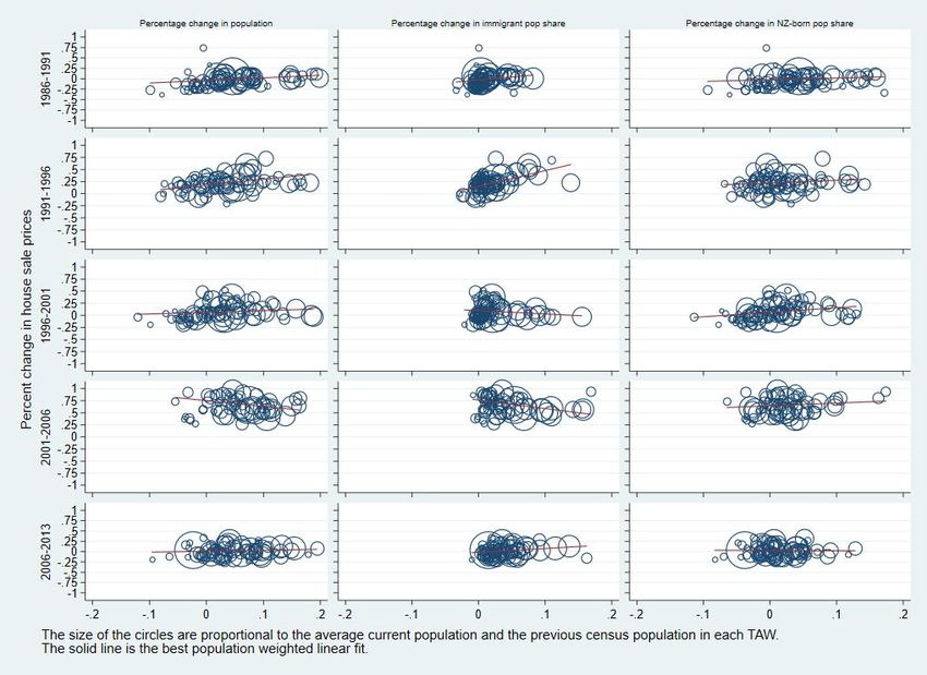
Housing markets and migration – Evidence from New Zealand

other groups are somewhere in between. Of interest is that, although the average age of
returning New Zealanders is similar to that of new immigrants, they have much higher rates of
home ownership. There are also differences in the household composition of the different
subpopulations: for example, new immigrants live in larger households which suggests that each
new immigrant may contribute relatively less to housing demand. These differences suggest that
each group may differentially affect house prices, and/or affect segments of the housing market,
such as home-ownership versus renting. To flexibly allow for different population effects in our
analysis, we will examine different housing market segments separately, and also control for
socio-economic characteristics of the subpopulations.

3.4 Exploratory analysis of house prices and population
In order to provide something of a cross-walk to the macroeconomic time series literature
(Coleman and Landon-Lane 2007; McDonald 2013) and our local area analysis, we begin with a
descriptive analysis of the relationships between population and house price changes. This
involves first graphical description, and second regression analysis, of the relationships.
 In Figure 2 and Figure 3 we describe the relationship between intercensal house price and
population changes: Figure 2 pools the inter-censal periods, while Figure 3 plots relationships
separately for each period. The top row of Figure 2 summarises the aggregate changes in house
prices versus total population (column 1), and foreign-born (immigrant) and New Zealand born
populations in columns 2 and 3 respectively. The first two graphs show similar strong aggregate
times series relationships between house price changes and total population or immigrant-
population changes (of 12 percent and 10 percent in response to a 1 percent population change
respectively) to those reported by Coleman and Landon-Lane (2007) and McDonald (2013);
while the third graph shows no relationship between price changes and NZ-born population
changes.
 The second row of Figure 2 disaggregates the aggregate house price and population data
to the local (TAW) level and presents scatterplots of local average price changes against
population changes. The size of each data-circle is proportional to the average local-area
population across consecutive censuses, while the (red) line gives the population-weighted
linear fit of the data. Pooled across census periods, this shows a much weaker local-area house
price versus population change relationship than in the aggregate data: the estimated price
elasticities with respect to the full population is 1.0, and with respect to the immigrant and NZ-
born populations is 1.9 and 0.6 respectively.
 To see whether areas whose populations grow relatively faster than the national average
have higher house price growth, the final row of Figure 2 plots the local average price changes
against population changes relative to the aggregate changes in each period. This again shows a
weaker local-area house price versus population change relationship, with estimated price

 10

Housing markets and migration – Evidence from New Zealand

elasticities of 0.3, 0.1, and 0.5 with respect to the full population, immigrant, and NZ-born
populations respectively. In this case the relationship between price and immigrant changes is
statistically insignificant, so the overall population effect appears to be most strongly associated
with local-area NZ-born population changes.
 To clarify the separate census-period patterns, Figure 3 disaggregates the scatterplots
from row 2 of Figure 2, separately by census period. These graphs clearly show strikingly
different patterns of both (higher) price and population changes between 2001 and 2006 than
the other inter-censal periods. In addition, the local-area weighted-average relationship between
either total population or immigrant population change and average house price change was
negative in this period, compared to generally mild positive relationships for other periods.
 We next provide an exploratory regression analysis of the relationship between local-area
and (aggregate) New Zealand population and local-area house prices.19 For this, we use TAW-
level data from the 1986–2013 censuses, and summarise the results in Table 3. Regression
results for house prices in levels (logarithms) are presented in panel (A), and results for house
price log-changes in panel (B). In column (1) we present results from simple regressions on
log(local area population): the estimates are each positive and significant, implying local-area
population elasticities of 0.3 in levels and 0.92 in changes. We next include log(NZ population),
which has large positive coefficients in both the level (3.2) and change (9.9) regressions: in fact,
the estimated log-change regression coefficient of 9.9 is in the range of long-run elasticities that
Coleman and Landon-Lane (2007) estimate. In addition, although the estimated local-area
population coefficients in column (2) remain positive and statistically significant, they are
somewhat lower than in column (1), particularly in the log-change regression. Consistent with
the pattern of results seen in Figure 2 and Figure 3, this is suggestive of omitted variable bias
inflating the population elasticities.
 In column (3) we include census-year fixed effects to control for aggregate effects common
across areas, which also absorbs the aggregate population variable. There are two comments of
note from this specification. First, the local-area population elasticities are the same as in
column (2), implying any coefficient ‘bias’ from omitted aggregate effects are adequately
controlled by the aggregate population variable. Second, as measured by its contribution to the
increase in the R-squared associated with the year fixed effects between columns (1) and (3)
regressions, population is a substantial contributor (or proxy for) unobserved aggregate factors
– i.e. it accounts for 92% of the increase in level-regression R-squared, and 50% of the increase
in the log-change R-squared.
 Finally, in columns (4) and (5), we report results for regressions that correspond to our
‘preferred’ specifications discussed in section 5.1 below, including either census-year fixed

19Coleman and Landon-Lane (2007) and McDonald (2013) focus on the link between migration (rather than
population) and house prices: nonetheless, this exploratory analysis is informative.
 11

Housing markets and migration – Evidence from New Zealand

effects (column (4)) or log(NZ population) (column (5)).20 The results in ‘levels’ imply that,
controlling for other area-level characteristics, the (column (5)) effects of both local and
aggregate population on local-area house prices are smaller (particularly the coefficient on
aggregate population) than reported in column (2) and no longer statistically significant. In
contrast, the ‘changes’ estimates are broadly similar to the simple regression estimates, with
larger local area population elasticities of 0.5–0.6, and only a slightly smaller aggregate
population elasticity of 8.7 in column (5).
 As expected, this descriptive analysis demonstrates that aggregate population is strongly
associated with local-area house prices, and also accounts for a large fraction of the variation
associated with the census-year fixed effects. Because of the possible confounding
macroeconomic factors associated with this variation, in what follows we abstract from these
effects and focus on the relationship between housing and population effects at the local-area.

4 Model framework
In this section we briefly outline the conceptual framework used to analyse the relationship
between alternative measures of housing demand and supply, and population growth and
immigration, and then derive the empirical specification used in the analysis. This begins with a
stylised structural supply and demand system for housing, from which we derive reduced-form
equations used to estimate the relationship between measures of the price and quantity of
housing, and population and other exogenous variables in the system. The framework will be
applied at the local area level separately for both Territorial Authorities and Auckland Wards
(TAW), and Labour Market Areas (LMA), and within these also to different housing market
segments – i.e. stratified by houses versus apartments, and sales versus rental markets.
 We posit that a local housing market can be characterised by demand for, and supply of,
housing equations as follows:
 
 = . + . + ′ . + , (1a)

 = . + ′ . + , (1b)

where and represent the quantity of housing demanded and supplied in local market-j in
year-t, is a measure of the price of housing, is (possibly) a vector of variables capturing
the population size and composition effects on housing demand, and and are vectors of
other exogenous variables that affect local housing demand and supply respectively.21 In this
framework, we expect the price effects on housing demand ( ) and supply ( ) to be negative

20 Our preferred ‘changes’ specification estimates presented here are based on all available observations, in contrast
to those in section 5.1 which are based on a balanced panel sample.
21 For emphasis and focus, we include the population variable(s) explicitly in the demand equation, separately from

the other exogenous variables .

 12

Housing markets and migration – Evidence from New Zealand

and positive respectively: i.e. all else equal, when the price of housing is higher, we expect less
demand, perhaps in the form of smaller houses; while supply will increase, because it will be
more attractive to supply housing. We also expect that population size will increase housing
demand, so the coefficient ( ) will be positive. Other variables that are likely to affect housing
demand even controlling for the size of the population include the socio-demographic and
economic characteristics of the local population, such as the marital status, age, qualification,
employment, and household size. Similarly, we will use building consent information on
alterations relative to new-buildings as controls to proxy for regulations and/or geographical
constraints on housing supply.
 Equations (1a) and (1b) represent the demand and supply structural equations for the
housing market. Assuming housing markets are in equilibrium then the realised price and
quantity of housing observed at any point in time represent the equilibrium price ( ) and
quantity ( ). Our primary interest is understanding the relationship between housing prices
and rents and population changes; and our secondary focus is on the responsiveness of housing
(supply) to population changes. For these purposes, we derive the (so-called) reduced-form
equations for the price and quantity, in terms of all the exogenous variables, as follows:

 − − 
 = . − ′ . + ′ . +
 − − − − 

 = . + ′ . + ′ . + 
 
 (2a)

 − − 
 = . − ′ . + ′ . +
 − − − − 
 
 = . + ′ . + ′ . + (2b)

where the . And . are the reduced-form coefficients on the exogenous variables affecting
 
housing demand or supply, and and are residuals, which depend on the structural
equation parameters and errors. Given the expected signs of the structural coefficients ( >
0, < 0, > 0), the reduced-form relationships between price and population, and between
quantity and population, in equations (2a) and (2b) will each be positive ( > 0, > 0).
 Our empirical analysis below will focus on specifications of these reduced-form equations
for housing prices and quantities. It is important to realise that the adequacy of these reduced-
form equations will depend on the adequacy of the structural equations (1a and 1b) and market
equilibrium assumptions. For example, if the structural equations are misspecified due to the
omission of relevant variables, such misspecification will also flow through to the reduced-form
equations (2a and 2b) and affect the estimation of these equations.
 Following Stillman and Maré (2008), we assume the basic relationship between the price
of housing and population involves log-log specifications for quantities, prices and population in

 13

Housing markets and migration – Evidence from New Zealand

both the demand and supply equations. For demand shifters, we include control variables for the
average socio-demographic and physical characteristics of the households in an area.22 For
supply shifters, we use information on building consents to proxy for regulation and/or physical
constraints on supply in an area. Our main variable in this regard is the share of housing
consents that are for new-build houses and apartments rather than extensions, which we
interpret as affecting the relative supply flexibility in an area. For example, we expect this share
variable will be higher in areas with more flexible regulations or less binding geographic
constraints that facilitate an increase in the quantity of available housing at lower marginal
cost.23 As the available information on factors that affect housing demand and supply is limited,
we will also use area-level fixed effects to control for constant unobserved differences across
areas.
 For brevity of notation, we combine the main population size (log(Pop)) and composition
(population-share) variables of interest, and denote these simply as log⁡( ) and summarise
the combined set of demand and supply control variables in the vector ′ . The main reduced-
form regressions of interest are expressed in levels as:

 log( ) = . log( ) + ′ . + 
 
 (3a)

 log( ) = . log( ) + ′ . + . (3b)

 In our analysis of the relationship between population and house prices and rent, we will
consider various extensions to the basic specification of equations (3a and 3b), to allow the
relationship between the price of housing and population to vary with either population growth,
perhaps reflecting short term supply constraints, and/or the immigrant versus native mix of the
population, perhaps reflecting heterogeneous housing demand across such sub-populations. We
will also consider estimating regressions for alternative specifications of equations (3a and 3b)
in levels, including area-level fixed effects to control for persistent differences in house prices
and rents across areas that are not adequately controlled for by observed factors; and also in
first-differences between census years.
 As discussed in section 3.3, to flexibly allow differential population effects across the
housing market, we will estimate separate reduced form price equations for the various house
versus apartments and sales-price versus rental housing market segments. However, we will
estimate reduced form quantity equations just for the combined market.

22 The physical characteristics (such as the number of bedrooms), in particular, can be thought of as providing hedonic
regression adjustments for house prices or rents.
23 In contrast, areas where the share of new-builds are lower because of with more stringent regulations that inhibit

new builds, and may result in increases in the relative quality of the housing stock. Our analysis does not control for
such quality changes, e.g. through a hedonic housing adjustment.
 14

Housing markets and migration – Evidence from New Zealand

5 Analysis and results
Our initial focus is on residential house prices as the primary outcome (dependent) variable, and
conduct the analysis using TAW-level observations. We then consider corresponding results for
the other housing outcomes of interest (the number of dwellings, price of apartments, rents of
houses, and rents of apartments), and alternative LMA-level observations.

5.1 Residential house prices
We now turn to our main house price regressions for equation (3a) in levels using TAW-level
data, which are summarised in Table 4. The first specification, in column (1), simply regresses
the logarithm of average house prices, log(House prices), on log(Adult population) , as well as
the share of the number of building consents for housing units that are for new (houses and
apartments) as opposed to alterations as a housing supply shifter proxy for supply constraints
due to (e.g.) building regulations or land availability, and census-year fixed effects using all
available observations over the period 1991–2013.24 The estimated coefficient on
log(population) is +0.25 and statistically significant, and implies, controlling for general house
price differences across census years, that house prices are about 2.5% higher in areas with 10%
higher population. To the extent that the new-build share measure is a positive supply-shift
proxy, we would expect it to positively affect housing quantity and negatively affect prices: in
contrast, the estimated effect of this measure on house prices is positive but not statistically
significant.
 To examine whether there are heterogeneous population effects on the price of housing
related to the immigration versus native mix of the population, in column (2) we include the
fractions of the population that are (since the last census) new immigrants, returning New
Zealanders, moving immigrants, moving New Zealanders, and staying immigrants.25 In this
specification the log(Pop) coefficient is substantially lower, and implies house prices are on
average 1% higher in areas with 10% higher population(from ‘staying New Zealanders’, the
omitted population-share category). The included population-share variables are each positive,
suggesting these other subpopulations have greater effect on house prices, although only the
‘returning New Zealanders’ and ‘moving immigrants’ coefficients are statistically significant. For
example, in areas with a 1% (0.01) higher share of returning New Zealanders (and 1% fewer
staying New Zealanders), house prices are about 29% higher on average, in addition to any

24 This building consents measure is calculated over the period between census dates, and may be (conceptually)
better suited to a house price change specification, with its ‘integrated equivalent’ measure used in the log (level)
specification. In the absence of such an integrated measure, we will include this measure in both the levels and
changes specifications.
25 Together with the fraction of staying (i.e. non-migrating) New Zealanders (the omitted category), these fractions

sum to 1.
 15

Housing markets and migration – Evidence from New Zealand

population-size (main) effect.26 Similarly, an area with a 1% redistribution of population from
staying New Zealanders to moving immigrants has about 6.7% higher house prices. The
estimated coefficient on the new-build consent share is now significant: a 10% increase in the
new-build share increases house prices by 3.2% on average.
 In column (3), we include controls for various observable socio-demographic
characteristics. Including these controls, has a small effect on the population size coefficient
(which falls about 10% to 0.09), but substantially reduces most of the coefficients on the
population-composition shares. As discussed above, these effects are consistent with the
composition subgroups having observably different characteristics that systematically affect
their demand for housing.
 To allow for possible dynamic responses of house prices to population growth, we next
include population growth (Δ log( ) = log( ) − log⁡( −1 )) in the regression. In
column (4) we include just Δ log( ) to the regression, and in column (5) we also include the
changing shares of the population subgroups. The results from these regressions are comparable
to those in column (3) and imply that neither population growth nor composition changes have
noticeable effects on house prices. The absence of dynamic responses suggests the analysis
based on the census-timing of the data provides long run estimates of the relationship between
population and house prices.
 The results in columns (6) – (8) are for regressions that include TAW fixed effects to
control for constant unobserved differences across areas. We first exclude the population
growth and change in population shares (column (6)), then include these variables (column (7)).
Including the area fixed effects results in a statistically significant estimated log(population)
coefficient of 0.29–0.3 and appears to absorb much of the population share effects, as well as the
population growth effects. This suggests that (e.g.) the large and significant returning New
Zealanders and moving immigrant share effects observed earlier are largely associated with
these groups moving into areas with higher average house prices. Based on these results, we
adopt the specification in column (6) as our preferred ‘levels’-specification.
 Finally, for consistency of samples across other outcomes, we re-estimate the preferred
regression specification (column (6)) on the sample restricted to a balanced panel of TAWs
observed from 1996 to 2013 and with no missing observations between 1991 and 2013.27 The
results from this regression, presented (in bold) in column (8), imply that areas with 10%
higher population have 3.9% higher house prices on average, controlling for observable
covariates and fixed unobservable factors, while there is no strong evidence that population
effects vary systematically across population subgroups. In fact, these results imply that a higher

26 Strictly speaking, the reported coefficient of 0.29 implies the average log(price) is 0.29 log-points higher in areas
with 1% more returning New Zealanders, which transforms to 34% higher house prices. To simplify the discussion,
we will interpret such log-point effects as “percentage” effects.
27 This will provide a consistent sample to compare results with those estimated in differences, as well as to those of

other outcomes (numbers of dwellings and apartment prices).
 16