ROOTS: Object-Centric Representation and Rendering of 3D Scenes

ROOTS: Object-Centric Representation and Rendering of
 3D Scenes

 Chang Chen∗ chang.chen@rutgers.edu
 Department of Computer Science
 Rutgers University
 Piscataway, NJ 08854, USA
 Fei Deng∗ fei.deng@rutgers.edu
 Department of Computer Science
arXiv:2006.06130v3 [cs.LG] 1 Jul 2021

 Rutgers University
 Piscataway, NJ 08854, USA
 Sungjin Ahn sungjin.ahn@rutgers.edu
 Department of Computer Science and Center for Cognitive Science
 Rutgers University
 Piscataway, NJ 08854, USA

 Abstract
 A crucial ability of human intelligence is to build up models of individual 3D objects from
 partial scene observations. Recent works achieve object-centric generation but without the
 ability to infer the representation, or achieve 3D scene representation learning but without
 object-centric compositionality. Therefore, learning to represent and render 3D scenes with
 object-centric compositionality remains elusive. In this paper, we propose a probabilistic
 generative model for learning to build modular and compositional 3D object models from
 partial observations of a multi-object scene. The proposed model can (i) infer the 3D object
 representations by learning to search and group object areas and also (ii) render from an
 arbitrary viewpoint not only individual objects but also the full scene by compositing the
 objects. The entire learning process is unsupervised and end-to-end. In experiments, in
 addition to generation quality, we also demonstrate that the learned representation permits
 object-wise manipulation and novel scene generation, and generalizes to various settings.
 Results can be found on our project website: https://sites.google.com/view/roots3d
 Keywords: object-centric representations, latent variable models, 3D scene generation,
 variational inference, 3D-aware representations

 1. Introduction
 At the core of human learning is the ability to build up mental models of the world along with
 the growing experience of our life. In building such models, a particularly important aspect
 is to factorize underlying structures of the world such as objects and their relationships. This
 ability is believed to be crucial in enabling various advanced cognitive functions in human-like
 AI systems (Lake et al., 2017) such as systematic generalization (Bahdanau et al., 2019; van
 Steenkiste et al., 2019), reasoning (Bottou, 2014), and causal learning (Schölkopf, 2019; Peters

 ∗. Both authors contributed equally.

 1

et al., 2017). While humans seem to learn such object-centric representations (Kahneman
et al., 1992; Rolls et al., 2005; Hood and Santos, 2009; von Hofsten and Spelke, 1985; Martin,
2007; Høydal et al., 2019) in a 3D-aware fashion through partial observations of scenes
without supervision, in machine learning this problem has only been tackled for simple 2D
fully-observable images (Eslami et al., 2016; Lin et al., 2020; Crawford and Pineau, 2019;
Greff et al., 2017, 2019; Locatello et al., 2020; Burgess et al., 2019; Engelcke et al., 2020).
Therefore, the more challenging yet realistic setting of learning 3D-aware object-centric
representation of 3D space from partial observations has remained elusive.
 Regarding this, there have been a number of recent approaches that can (only) generate
3D scene images via object-centric compositional rendering (Nguyen-Phuoc et al., 2020;
van Steenkiste et al., 2020; Ehrhardt et al., 2020). However, none of the existing models
provide the crucial ability of the reverse that we seek in this paper: the object-centric
inverse graphics, i.e., learning object-centric 3D representations from partial observations.
In learning representations and rendering of 3D scenes, GQN (Eslami et al., 2018) and its
variants (Kumar et al., 2018; Tobin et al., 2019; Singh et al., 2019; Yoon et al., 2020) are the
most close to our work. However, the 3D representations inferred by these models provide
only scene-level representation without explicit object-centric decomposition.
 In this paper, we tackle the problem of learning to build modular and compositional 3D
object models from partial scene images. Our proposed model, ROOTS (Representation and
 ¯
Rendering of Object-Oriented Three-D Scenes), is able to decompose partial observations
 ¯ ¯ ¯ ¯
into objects, group them object-wise, and build a modular compositional 3D representation
at the level of individual objects. Such representation also enables compositional rendering.
As our object model provides object-wise 3D rendering from arbitrary viewpoint, we can
also render the entire scene from arbitrary viewpoints by first rendering individual objects
and then compositing them according to the scene layout. In particular, this enables a
novel nested autoencoder architecture in which we can reuse the GQN model as a internal
autoencoder module for object modeling, making the model simpler. The entire process is
unsupervised and end-to-end trainable. We demonstrate the above capabilities of our model
on simulated 3D scenes with multiple objects. We evaluate our model in terms of generation
quality, structure accuracy, generalization ability, and downstream task performance. We
also showcase that by manipulating the scene layout, we can generate scenes with many
more objects than typical of the training regime.

2. Preliminary: Generative Query Networks

The Generative Query Network (GQN) is a latent variable model for learning to represent
and render 3D scenes. Given a set of context images and viewpoints, it learns a 3D-
viewpoint-steerable representation (in short, 3D representation throughout this paper) in the
sense that any target image viewed from an arbitrary viewpoint can be generated from the
representation. We note that such 3D representations are different from and more challenging
to learn than 2D representations that only model the scene from a single viewpoint. Recent
advances in unsupervised object-centric representation learning (Eslami et al., 2016; Lin
et al., 2020; Crawford and Pineau, 2019; Greff et al., 2017, 2019; Locatello et al., 2020;
Burgess et al., 2019; Engelcke et al., 2020) mostly require the representation to model only

 2

a single 2D image. Therefore, these methods can only learn 2D representations, even if the
2D image is a view of an underlying 3D scene.
 More formally, consider an agent navigating a 3D environment (called a scene) and
collecting K pairs of image xc and the corresponding viewpoint vc for c = 1, 2, . . . , K. This
collection is called context C = {(xc , vc )}K
 c=1 . GQN learns a scene-level 3D representation z
by encoding C, such that the target image x̂q from an arbitrary query viewpoint vq can be
generated by the decoder x̂q = GQNdec (z, vq ). The generative process can be written as:
 Z
 p(xq | vq , C) = p(xq | z, vq ) p(z | C) dz .

The prior encoder p(z | C) = GQNenc (C) first obtains an order-invariant encoding (e.g., a sum
encoding) rC of context C, and then uses ConvDRAW (Gregor et al., 2016) to autoregressively
sample z from rC . The decoder GQNdec (z, vq ) uses a deterministic version of ConvDRAW
to render the target image x̂q from z, and p(xq | z, vq ) is often modeled as a Gaussian
distribution N (x̂q , σ 2 1) with σ being a hyperparameter. Since computing the posterior
distribution p(z | xq , vq , C) is intractable, GQN uses variational inference for posterior
approximation and is trained by maximizing its evidence lower bound. Backpropagation
through random variables is done by the reparameterization trick (Kingma and Welling,
2014; Rezende et al., 2014).
 Note that the model described above is actually a more consistent version of the GQN
named CGQN (Kumar et al., 2018). In the original GQN (Eslami et al., 2018), the latent
z is also conditioned on vq , i.e., p(z | vq , C), and rendering is query-agnostic, i.e., p(xq | z),
leading to potential inconsistency across multiple query viewpoints. Throughout the paper,
we use the abbreviation GQN to refer to the general GQN framework embracing both GQN
and CGQN.

3. ROOTS
GQN represents a multi-object 3D scene as a single vector without learning explicit object-
wise decomposition. Hence, it cannot entertain the potential and various advantages of
object-centric representations. To resolve this limitation, we propose ROOTS, a probabilistic
generative model that learns to represent and render 3D scenes via composition of object-
centric 3D representations in a fully unsupervised and end-to-end trainable way. This
problem has never been tackled, and it is highly challenging because not only can an object
be unobservable from certain viewpoints, but also the appearance, position, pose, size, and
occlusion of an object can vary significantly across the context images. The premise of our
approach to tackling this challenge is that: if we can collect the local regions corresponding
to a specific object across the context images, then we can reuse GQN on those filtered local
observations to learn the 3D representation for that object.
 To this end, we propose the following approaches. First, ROOTS has a nested autoencoder
architecture, one autoencoder at scene-level and the other at object-level. Further, the scene-
level autoencoder is constructed by the composition of the object-level autoencoders. For
the scene-level encoding, the model encodes the context set to a 3D spatial structure of the
scene and infers the 3D position of each object existing in the 3D space. Given the inferred
3D position of objects, we then propose a method, called Attention-by-Perspective-Projection

 3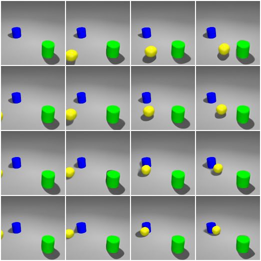

ROOTS Encoder !"# ROOTS Decoder

 v1 vq
 v1 v2
 !
 vq

 + +
 v2 vq
 v1 v2
 " v1
 v2

 (a) Scene Encoding (b) Obj-Attention Grouping (c) Obj-Level Contexts (d) Obj Models (e) Obj Rendering (f) Scene Composing

Figure 1: Overview of ROOTS pipeline. ROOTS encoder (a - c): (a) Context observations
 are encoded and aggregated into a scene-level representation ψ. (b) ψ is reor-
 ganized into a feature map of the 3D space, from which 3D center positions are
 inferred for each object. By applying perspective projection to the inferred 3D
 center positions, we identify image regions for each object across viewpoints. (c)
 Object regions are cropped and grouped into object-level contexts. Object models
 (d): The object-level contexts allow us to obtain the 3D appearance representation
 of each object through an object-level GQN. ROOTS decoder (e - f ): To render
 the full scene for a given query viewpoint, we composite the rendering results of
 individual objects.

to efficiently find and attend the local regions, corresponding to a specific object, across
all the context images. This grouping allows us to construct a new object-level context
set containing only a specific object and thus to reuse the standard GQN encoder as an
in-network module for object-level 3D-aware encoding of the object appearance. Scene-level
decoding is also composed by object-level decoding and background-decoding. We decode
the appearance representation of each object using the object-level GQN decoder, and place
the decoded images in the target image by mapping the 3D positions to the 2D positions in
the target image. Together with background rendering, we can complete the rendering of a
scene image. See Figure 1 for an overview of ROOTS pipeline.

3.1 ROOTS Encoder
The goal of ROOTS encoder is to infer the 3D object models from scene-level context
observations C = {(xc , vc )}K
 c=1 but without any object-level supervision. Each object model
consists of the 3D representation of an object, fully disentangled into its 3D position and 3D
appearance. The modularity and compositionality of these object models allow them to be
collected from multiple scenes, and then reconfigured to generate novel scenes that are out
of the training distribution.
 To infer the 3D object models, it is imperative that the encoder should be properly
structured. In particular, we find in our experiments that directly inferring object models
from an order-invariant encoding of C would fail, potentially because the lack of proper
structure prohibits learning and optimization. To solve this problem, we extract object

 4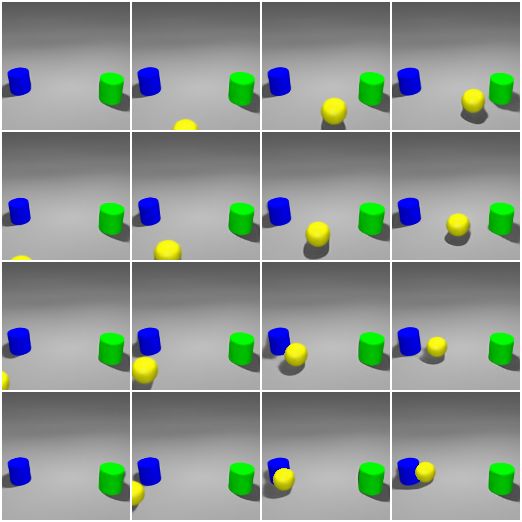

regions from each scene image xc and group them into object-level contexts, which provide
more relevant information for inferring the 3D appearance of each object. We call this
grouping process object-attention grouping.
 For 2D fully observable images, extracting object regions can be solved by recent 2D
scene decomposition methods (Eslami et al., 2016; Crawford and Pineau, 2019; Lin et al.,
2020). However, in our 3D and partially observed setting, it remains a challenge to efficiently
group together the regions that correspond to the same object across viewpoints. One
naive approach is to find the best among all possible groupings, but its time complexity is
exponential in the number of viewpoints. Another possible way is to treat the extracted
object regions in one viewpoint as anchors, and match regions from other viewpoints to one
of these anchors, by computing pairwise matching scores. The time complexity is quadratic
in the number of objects. By contrast, our proposed object-attention grouping scales linearly
in both the number of viewpoints and the number of objects. The key idea is to first infer
the center position of each object in 3D coordinates. This allows us to use perspective
projection (Hartley and Zisserman, 2003) from 3D to 2D to efficiently locate the same object
across different context images.
 We develop a scene encoder (Section 3.1.1) to infer the object positions, describe in more
detail the object-attention grouping in Section 3.1.2, and use an object-level GQN encoder
(Section 3.1.3) to infer the object appearance.

3.1.1 Scene Encoder
The goal of the scene encoder is to infer the 3D center position of each object in world
coordinates—the same coordinate system where the camera viewpoints vc are measured. We
assume that the objects resides in a bounded 3D space. The scene encoder partitions this
bounded 3D space into a rectangular cuboid of Nmax = Nx × Ny × Nz cells. For each cell
(i, j, k), we infer a Bernoulli variable zpres
 ijk ∈ {0, 1} that is 1 if and only if the cell contains the
center of an object (note that the full appearance volume of an object need not be contained
within the cell). We also infer a continuous variable zwhere
 ijk ∈ R3 that, when zpres
 ijk = 1, specifies
 where
the center position of the object in the 3D world coordinates. Here zijk is constrained
to be within the boundary of cell (i, j, k). This prior on cell-wise object preference helps
efficient training and obviates the need for expensive autoregressive processing (Lin et al.,
2020).
 In the above scene encoding, each cell handles one or no object. In actual implementation,
however, the partition is soft, meaning neighboring cells can have some overlap. Hence,
when a cell does contain more than one object, the scene encoder can learn to distribute
them to adjacent cells. We can also simply increase the resolution of the 3D partitioning. A
similar 2D version of this approach has been used in SPAIR (Crawford and Pineau, 2019)
and SPACE (Lin et al., 2020), showing impressive decomposition of 2D scenes into dozens
of objects.
 Specifically, to infer {(zpres where
 ijk , zijk )} from the context observations C, we encode C into
a Geometric Volume Feature Map (GVFM) r ∈ RNx ×Ny ×Nz ×d , yielding a d-dimensional
feature vector rijk for each cell. Then, {(zpres where
 ijk , zijk )} can be computed in parallel for all
cells by a neural network fpres,where :

 p(zpres where
 ijk , zijk
 neighbor
 | C) = fpres,where (rijk ),

 5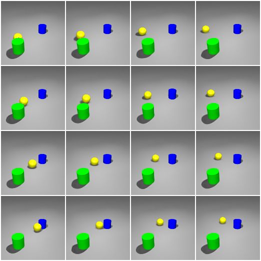

neighbor
where rijk includes the feature vectors of cell (i, j, k) and its neighboring cells, allowing
inter-object relations to be taken into consideration.
 While GVFM may seem similar to the grid cells used in SPAIR and SPACE, there
are fundamental differences. As a feature map of the 3D space, GVFM must aggregate
information from multiple partial 2D observations and reorganize it in an object-wise fashion.
This is in contrast to the 2D feature map learned by grid cells which have a natural alignment
with the single fully-observed 2D image. Therefore, we obtain GVFM in two steps. First, we
compute an order-invariant summary ψ of C as the summation over encodings of individual
context observations:
 ψ= K
 P PK
 c=1 ψc = c=1 fψ (xc , vc ) ,
where fψ is a learned encoding network. Second, we apply a 3D transposed convolution over
ψ to turn the sum of 2D image representations ψ into 3D spatial representation r where
individual rijk slots contains object-specific information:
 r = ConvTranspose3D(ψ) .

3.1.2 Object-Attention Grouping
Object-attention grouping aims to identify image regions that correspond to the same object
across different observation images. This is crucial in obtaining object-wise 3D appearance
representations. More precisely, for each object n present in the scene and each context image
xc , we seek a 2D bounding box capturing object n in xc . The bounding box is parameterized
by its center position and scale (width and height), denoted (ocenter scale
 n,c , on,c ). Notice that here
each object index n corresponds to a distinct cell index (i, j, k) with zpres
 ijk = 1.
 Our key observation is that inferring the 3D object center positions in the first step
allows us to solve object-attention grouping by using perspective projection. We call this
Attention-by-Perspective-Projection (APP). Assuming that the projection operation takes
constant time, the time complexity of APP is linear in both the number of objects and the
number of viewpoints.
 Attention-by-Perspective-Projection (APP). Let us focus on object n and find its
2D bounding box in xc . We first analytically compute its 2D center position ocenter
 n,c ∈ R2 in
xc and its distance from the camera, denoted odepth
 n,c ∈ R, by applying perspective projection
to its 3D center position znwhere :
 depth >
 [ocenter where
 n,c , on,c ] = APPpos (zn , vc ) = normalize(TWorld→Camera (vc )[zwhere
 n , 1]> ) .

Here, zwhere
 n is first converted to camera coordinates by the viewpoint-dependent transfor-
mation matrix TWorld→Camera (vc ) ∈ R3×4 , and then normalized. See Appendix D for more
details.
 To compute the 2D bounding box scale oscale 2
 n,c ∈ R , one option is to learn a 3D bounding
box for object n, project its eight vertices onto the image plane, and find the smallest
rectangle that covers all eight vertices. Unfortunately, the resulting 2D bounding box will
only be tight under specific viewpoints, and we will likely encounter optimization difficulties.
Hence, to allow better gradient flow and provide the model with the opportunity to predict
tighter 2D bounding boxes, we design APPscale that implicitly learns the projection:
p(oscale where
 n,c | zn , C) = APPscale (ocenter depth center depth
 n,c , on,c , rn , vc ) = MLP(concat[on,c , on,c , rn , vc ]) .

 6

To work properly, APPscale should learn to perform the following operation implicitly: to
extract 3D scale information from rn , make a projection from viewpoint vc , and refine the
projection using ocenter
 n,c and odepth
 n,c .

3.1.3 Object Encoder
With object-attention grouping, we can decompose the scene-level context C into object-level
context Cn for each object n = 1, 2, . . . , N , where

 N = ijk zpres
 P
 ijk ≤ Nmax

is the total number of objects present in the scene. Specifically, we first use a spatial
transformer ST (Jaderberg et al., 2015) to differentiably crop object patch xatt
 n,c from scene
image xc using ocenter
 n,c and o scale :
 n,c

 xatt center scale
 n,c = ST (xc , on,c , on,c ) .

After collecting these patches from all viewpoints, we group them based on the object index
n to obtain object-level context

 Cn = {(xatt where K
 n,c , vc , on,c )}c=1 ,

where we include owhere = (ocenter scale depth
 n,c n,c , on,c , on,c ) to provide information complementary to
xatt
 n,c . The object-level context allows us to use an object-level GQN encoder

 p(zwhat
 n | Cn ) = GQNenc (Cn )

to obtain independent and modular object-level 3D appearance zwhat
 n for each object n. A
summary of ROOTS encoder is provided in Appendix C.

3.2 ROOTS Decoder
Given partial observations of a multi-object 3D scene, ROOTS not only learns to infer
the 3D object models, but also learns to render them independently and individually from
arbitrary viewpoints. The full scene is also rendered from arbitrary query viewpoints by
compositing object rendering results. By collecting and re-configuring the inferred object
models, ROOTS can easily generate novel scenes that are out of the training distribution.
 Object Renderer. For each object n, given its 3D appearance representation zwhat n
and a query viewpoint vq , ROOTS is able to generate a 4-channel (RGB+Mask) image
owhat
 n,q depicting the object’s 2D appearance when viewed from vq . This is achieved by an
object-level GQN decoder:

 owhat what att
 n,q = GQNdec (concat[zn , rn ], vq ) .

Here, rnatt is an order-invariant summary of object-level context Cn :

 rnatt = K att where
 P
 c=1 fatt (xn,c , vc , on,c ) ,

where fatt is a learnable encoding network.

 7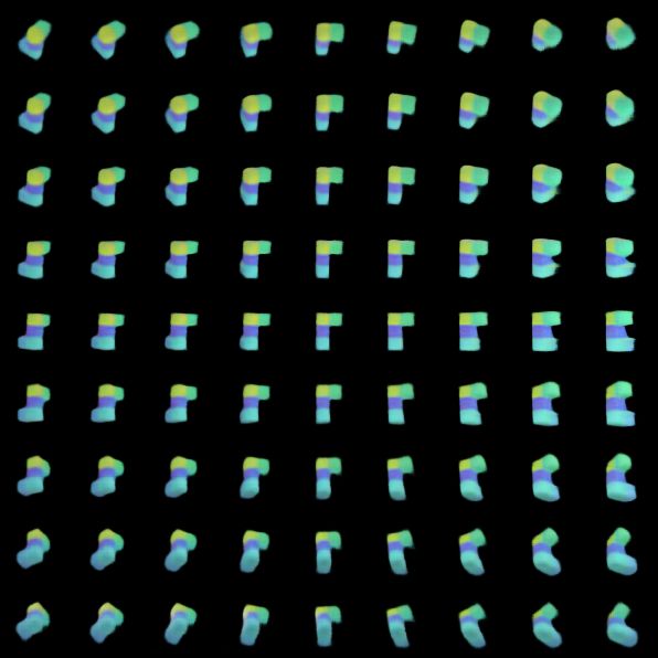

Scene Composer. The final scene image x̂q corresponding to query vq is obtained by
superimposing layers of object-wise images with proper masking. For this, we first use an
inverse spatial transformer ST −1 (Jaderberg et al., 2015) to differentiably place each object
at the right position in the scene canvas with proper scaling:

 [x̂n,q , m̂n,q ] = ST −1 (owhat center scale
 n,q , on,q , on,q ) .

Here, the 3-channel image x̂n,q can be regarded as an object-specific image layer containing
only object n, and the single-channel m̂n,q is the mask for object n. The position and scaling
parameters are computed by simply reusing the APP module for query viewpoint vq :
 depth >
 [ocenter where
 n,q , on,q ] = APPpos (zn , vq ) ,
 p(oscale where
 n,q | zn , vq , C) = APPscale (ocenter depth
 n,q , on,q , rn , vq ) .

We then composite these N image layers into a single image, ensuring that occlusion among
objects is properly handled. Similar to previous works (van Steenkiste et al., 2018; Crawford
and Pineau, 2019; Burgess et al., 2019; Greff et al., 2019; Engelcke et al., 2020; Lin et al.,
2020), for each layer n, we compute a transparency map

 αn,q = wn,q m̂n,q ,

where is pixel-wise multiplication. This masks out occluded pixels of object n. To
obtain the values of {wn,q }N N
 n=1 at each pixel, we first use {m̂n,q }n=1 to find the objects that
contain the pixel, and then assign the values based on their relative depth {odepth N
 n,q }n=1 . See
Appendix E for more details. The final rendered scene x̂q is composited as:
 PN
 x̂q = n=1 αn,q x̂n,q .

A summary of ROOTS decoder is provided in Appendix C.

3.3 Probabilistic Model
We now piece things together and formulate ROOTS as a conditional generative model.
Given a collection of context observations C = {(xc , vc )}Kc=1 of a multi-object scene, ROOTS
learns to infer the number of objects, denoted N , the 3D object model z3D n = (zn
 where , zwhat )
 n
for each object n = 1, 2, . . . , N , and the 2D representation o2D
 n,C = {o where }K collected for
 n,c c=1
each object n from all context viewpoints. In addition, ROOTS also learns a background
representation zbg through a scene-level GQN encoder:

 p(zbg | C) = GQNbg
 enc (C) .

Using these representations, ROOTS can then generate the target image xq from an arbitrary
query viewpoint vq of the same scene. During generation, ROOTS also infers the 2D object
representation o2D where for the query viewpoint. We do not include owhat here because
 n,q = on,q n,q
it is a deterministic variable.
 Let Q = {(xq , vq )}M M
 q=1 be the collection of queries for the same scene, xQ = {xq }q=1 and
 M
vQ = {vq }q=1 be the target images and query viewpoints respectively, and D = C ∪ Q be the

 8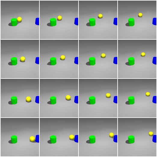

union of contexts and queries. To simplify notations, we collect all viewpoint-independent
3D representations into a single variable z3D , including the number of objects, the 3D object
models, and the background representation:

 z3D = (N, {z3D N bg
 n }n=1 , z ) .

We also collect the viewpoint-dependent 2D representations for all objects into a single
variable o2D
 S , where the subscript S denotes the set of viewpoints. For example,

 o2D 2D N
 C = {on,C }n=1 , o2D 2D N
 q = {on,q }n=1 .

The generative process can then be written as:
 ZZ M
 Y
 p(xQ | vQ , C) = p(z3D , o2D | C) p(o2D 3D 3D 2D 3D 2D
 q | z , vq , C) p(xq | z , oC∪q , vq , C) dz doD .
 | {zC }
 q=1
 | {z } | {z }
 Encoder Object Renderer Scene Composer

The encoder can be further factorized in an object-wise fashion:
 N
 Y
 3D
 p(z , o2D
 C | C)
 bg
 = p(z | C) p(N | C) p(zwhere | C) p(o2D | zwhere , C) p(zwhat | Cn ) ,
 | {z } | {z } | n {z } | n,C {zn }|
 n
 {z }
 n=1
 Background Density Scene Encoder APP Object Encoder

where the object-level context Cn is obtained as a deterministic function of zwhere
 n , o2D
 n,C , and
C. The object renderer can be factorized similarly:
 N
 Y
 p(o2D 3D
 q | z , vq , C) = p(o2D where
 n,q | zn , vq , C) .
 n=1
 | {z }
 APP

The scene composer obtains the full scene from the foreground image x̂q and the background
image x̂bg
 q through alpha compositing:
  PN 
 p(xq | z3D , o2D
 C∪q , v q , C) = N x̂ q + (1 − α
 n=1 n,q ) x̂ bg
 q , σ 2
 1 ,

where x̂bg
 q is rendered by a scene-level GQN decoder:

 bg
 x̂bg bg
 q = GQNdec (z , vq ) ,

and σ 2 is a hyperparameter called pixel-variance.

3.4 Inference and Learning
Due to the intractability of the log-likelihood log p(xQ | vQ , C), we train ROOTS using
variational inference with the following approximate posterior:
 N
 Y
 q(z3D , o2D bg
 D | D) = q(z | D) q(N | D) q(zwhere
 n | D) q(o2D where
 n,D | zn , D) q(zwhat
 n | Dn ) ,
 n=1

 9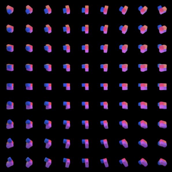

where Dn is the object-level context deterministically obtained from D using the inferred
zwhere
 n and o2Dn,D . The implementation of the approximate posterior is almost the same
as ROOTS encoder described in Section 3.1, except that the summary vector ψ should
now encode the entire D instead of only C. We treat all continuous variables as Gaussian
variables, and use reparameterization trick (Kingma and Welling, 2014) to sample from the
approximate posterior. For discrete variables, we use Gumbel-Softmax trick (Jang et al.,
2017; Maddison et al., 2017). The entire model can be trained end-to-end by maximizing
the Evidence Lower Bound (ELBO):
 hP i
 M
 L = Eq(z3D ,o2D |D) q=1 log p(xq | z3D , o2D
 C∪q , vq , C) − DKL [q(zbg | D) k p(zbg | C)]
 D
 hP i
 N 3D 2D 3D 2D
 − DKL [q(N | D) k p(N | C)] − Eq(N |D) n=1 DKL [q(zn , on,D | D) k p(zn , on,D | vQ , C)] .

 Combining with Unconditioned Prior. One difficulty in using the conditional
prior is that it may not coincide with our prior knowledge of the latent variables. In our
experiments, it turns out that biasing the posterior of some variables toward our prior
preference helps stabilize the model. We achieve this by introducing additional KL terms
between the posterior and unconditioned prior (like in VAEs, Kingma and Welling 2014;
Higgins et al. 2017) to the ELBO. Specifically, the model is trained by maximizing:
 hP i
 N where
 L̃ = L − γDKL [q(N | D) k Geom(ρ)] − Eq(N |D) D
 n=1 KL [q(zn | D) k N (0, 1)]
 hP i
 N 2D where
 − Eq(N |D) E where
 n=1 q(zn |D) [DKL [q(o |
 n,D nz , D) k N (0, 1)]] .

Here, γ is a weighting hyperparameter, and Geom(ρ) is a truncated Geometric distribution
with support {0, 1, . . . , Nmax } and success probability ρ. We set γ = 7 and ρ = 0.999 during
training, thereby encouraging the model to decompose the scenes into as few objects as
possible.

4. Related Work
ROOTS is broadly related to recent advances in learning representations for the appearance
and geometry of 3D scenes, and more closely related to those that do not require 3D
supervision. ROOTS is also inspired by recent works that learn to decompose 2D scenes
into object-wise representations.
 Geometric Deep Learning. Learning representations that capture the geometry of
3D scenes has been of growing interest. Recent works have explored integrating voxels
(Maturana and Scherer, 2015; Kar et al., 2017; Tulsiani et al., 2017; Wu et al., 2016; Choy
et al., 2016), meshes (Kato et al., 2018; Kanazawa et al., 2018), point clouds (Qi et al., 2017;
Achlioptas et al., 2018), and many other classical representations into deep learning models
to achieve better 3D scene understanding. However, they often require 3D supervision
(Huang et al., 2018; Tulsiani et al., 2018; Cheng et al., 2018; Shin et al., 2019; Du et al.,
2018) and work on single-object scenes (Wu et al., 2016; Yan et al., 2016; Choy et al., 2016;
Kar et al., 2017; Nguyen-Phuoc et al., 2019). By contrast, ROOTS learns to decompose a
multi-object scene into object-wise representations without any 3D supervision.
 Neural Representation of 3D Scenes. Recent works (Eslami et al., 2018; Kumar
et al., 2018; Tobin et al., 2019; Tung et al., 2019; Sitzmann et al., 2019a,b; Singh et al., 2019;

 10

Mildenhall et al., 2020; Dupont et al., 2020) have explored learning 3D scene representations
from 2D images without 3D supervision. While the rendering quality (Tobin et al., 2019;
Sitzmann et al., 2019b; Mildenhall et al., 2020) and efficiency (Dupont et al., 2020) have
been improved, these methods are not able to decompose the full scene into objects without
object-level supervision, and cannot learn object-wise representation and rendering models.
We believe these works are complementary to ROOTS and may allow object models to be
learned from more realistic scenes. Crawford and Pineau (2020) recently proposed to learn
3D object-centric representations from unlabeled videos. Although their model can infer the
3D position of each object, the object appearance is modeled in 2D. Another line of work
(Nguyen-Phuoc et al., 2020; Liao et al., 2020) learns object-aware 3D scene representations
for generative adversarial networks (Goodfellow et al., 2014). They only support rendering
and are unable to infer the object models for a given scene.
 Object-Oriented Representation of 2D Images. There have been prolific advances
in unsupervised object-oriented representation learning from fully-observed 2D images. They
mainly fall into two categories: detection-based and mixture-based. The detection-based
approaches (Eslami et al., 2016; Crawford and Pineau, 2019; Lin et al., 2020) first identify
object regions and then learn object representations from object patches cropped by the
spatial transformer (Jaderberg et al., 2015). The mixture-based approaches (Greff et al.,
2017; Burgess et al., 2019; Greff et al., 2019; Engelcke et al., 2020) model the observed image
as a pixel-level Gaussian mixture where each component is expected to capture a single
object. None of these approaches consider the 3D structure of the scene, let alone the 3D
appearance of objects.

5. Experiments
In this section, we evaluate the quality of object models learned by ROOTS and demonstrate
the benefits they bring in terms of generation quality, generalization ability, and downstream
task performance. We also showcase the built-in compositionality and disentanglement
properties of ROOTS. We first introduce the data sets and baselines we use, and then show
both qualitative and quantitative results.
 Data Sets. Existing data sets in previous work on unsupervised 3D scene representation
learning (Eslami et al., 2018; Tobin et al., 2019) either do not contain multi-object scenes or
cannot provide object-wise groundtruth information like object positions, and thus cannot
serve our purpose. Hence, we created two data sets: the Shapes data set and the Multi-
Shepard-Metzler (MSM) data set, using MuJoCo (Todorov et al., 2012) and Blender (Blender
Online Community, 2017) respectively. Both data sets contain 60K multi-object scenes
(50K for training, 5K for validation, and 5K for testing) with complete groundtruth scene
specifications. Each scene is rendered as 128×128 color images from 30 random viewpoints.
Notice that the scene specifications are for evaluation only and are not used during training.
 We generated three versions of the Shapes data set, containing scenes with 1-3, 2-4, and
3-5 objects respectively. The position, size, shape, and color of the objects are randomized.
The MSM data set contains scenes with 2-4 randomly positioned Shepard-Metzler objects.
Each object consists of 5 cubes whose positions are generated by a self-avoiding random
walk. The color of each cube is independently sampled from a continuous color space, as
described in GQN (Eslami et al., 2018). Since these objects have complex shapes randomly

 11

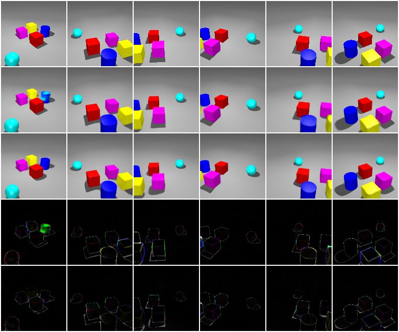
Target

 GQN

 ROOTS

 GQN-Err

 ROOTS-Err

Figure 2: Sample generations from three scenes. Columns correspond to query viewpoints.
 ROOTS gives better generations in regions of occlusion while GQN sometimes
 misses occluded objects and predicts wrong colors. GQN-Err and ROOTS-Err are
 difference maps between targets and generations of GQN and ROOTS, respectively.

generated per scene, they span a large combinatorial space, and it is unlikely that two
different scenes will share a same object. Also, the objects can have severe occlusion with
each other, making this data set significantly more challenging than the single-object version
considered in GQN.
 For evaluation on realistic objects, we also included a publicly available ShapeNet
arrangement data set (Tung et al., 2019; Cheng et al., 2018). Each scene of this data set
consists of 2 ShapeNet (Chang et al., 2015) objects placed on a table surface, and is rendered
from 54 fixed cameras positioned on the upper hemisphere. Following prior work, we split
the data set into a training set of 300 scenes and a test set of 32 scenes containing unseen
objects. Because object-wise annotations are not available, we did not perform quantitative
evaluation of object-level decomposition on this data set.
 Baselines. Because there is no previous work that can build 3D object models from
multi-object scene images, we use separate baselines to evaluate scene-level representation
and object-level decomposition respectively. For scene-level representation and generation
quality, we use CGQN (Kumar et al., 2018) as the baseline model, and refer to it as
GQN in the rest of this section to indicate the general GQN framework. For object-level
decomposition, we compare the image segmentation ability embedded in ROOTS with
that of IODINE (Greff et al., 2019), which focuses on this ability without learning 3D
representations.

5.1 Qualitative Evaluation
In this section, we qualitatively evaluate the learned object models by showing scene
generation and decomposition results and object model visualizations. We also demonstrate
the built-in compositionality and disentanglement properties by compositing novel scenes
out of the training distribution and visualizing latent traversals, respectively.

 12

Scene Generation. Like GQN, ROOTS is able to generate target observations for
a given scene from arbitrary query viewpoints. Figure 2 shows a comparison of scene
generations using 15 contexts. ROOTS gives better generations in regions of occlusion
(especially on the MSM data set), and correctly infers partially observable objects (e.g.,
the yellow cube in the 4th column). In contrast, GQN tends to miss heavily occluded and
partially observable objects, and sometimes predicts wrong colors. As highlighted in the
difference maps in Figure 2, on the Shapes data set, GQN sometimes generates inconsistent
colors within an object. On the MSM data set, GQN samples may look slightly clearer than
those of ROOTS as GQN generates sharper boundaries between the unit cubes. However,
the difference map reveals that GQN more frequently draws the objects with wrong colors.
On the ShapeNet arrangement data set, GQN samples are more blurry and also with wrong
colors. We believe that the object models learned by ROOTS and the object-level modular
rendering provide ROOTS with a stronger capacity to represent the appearance of individual
objects, leading to its better generation quality.
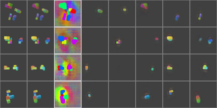
 Object Models. We further visualize the learned object models in Figure 4A, by
applying the object renderer to zwhat
 n and a set of query viewpoints. We also show the scene
rendering process in Figure 3, where object rendering results are composited to generate the
full scene. As can be seen, from images containing multiple objects with occlusion, ROOTS
is able to learn the complete 3D appearance of each object, predict accurate object positions,
and correctly handle occlusion. Such object models are not available from GQN because it
only learns scene-level representations.
 Compositionality. Once object models are learned, they can be reconfigured to form
novel scenes that are out of the training distribution. As an example, in Figure 4B, we first
provide ROOTS with context images from three scenes (top three rows) with 3 objects each,
and collect the learned object representations {(rnatt , zwhere
 n , zwhat
 n )}. A new scene with 9
objects can then be composed and rendered from arbitrary query viewpoints. Rendering
results are shown in the bottom row of Figure 4B. We would like to emphasize that the
model is trained on scenes with 1-3 objects. Thus, a scene with 9 objects has never been
seen during training.
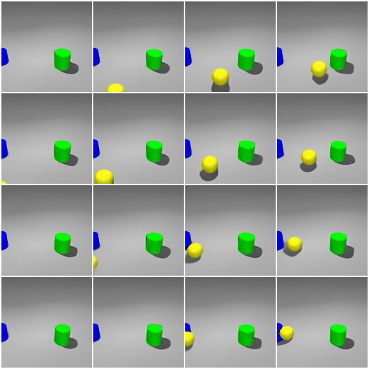
 Disentanglement. Since object position and appearance are disentangled in the learned
object models, by manipulating the position latent, we are able to move objects around
without changing other factors like object appearance. In Figure 5, we visualize traversals
of zwhere,x
 n and zwhere,y
 n of the yellow ball through generations from 5 query viewpoints. It
can be seen that the change of one coordinate does not affect the other. In addition, the
appearance of the yellow ball remains complete and clean during the traversal. Other
untouched components (the green cylinder, the blue cylinder, and the background) remain
unchanged. Moreover, we also notice some desired rendering effects. For example, the size
of the yellow ball becomes smaller as it moves further away from the camera.

5.2 Quantitative Evaluation

In this section, we report quantitative results on scene generation and decomposition, which
reflect the quality of the learned object models. We also highlight the benefit of learning
object models in two downstream tasks.

 13

Target Generation Decomposition

Figure 3: The full scene is composited from individual object rendering results. Predicted
 bounding boxes are drawn on target images.

 A Yaw B

 Pitch

Figure 4: (A) Visualization of learned object models from a set of query viewpoints. (B)
 Learned object models are reconfigured into a novel scene. Columns correspond
 to query viewpoints.

 14

-2 2
 2

 -2

 x

 y

Figure 5: Traversal of the position latent zwhere,x
 n and zwhere,y
 n of the yellow ball in the scene.
 We show generations from five query viewpoints after manipulating the position
 latent.

 Data Set 1-3 Shapes 2-4 Shapes 3-5 Shapes
 Metrics NLL↓ MSE↓ NLL↓ MSE↓ NLL↓ MSE↓
 ROOTS -207595.81 30.60 -206611.07 42.41 -205608.07 54.45
 GQN -206760.87 40.62 -205604.74 54.49 -204918.39 62.73

 Table 1: Quantitative evaluation of scene generation on the Shapes data sets.

 Scene Generation. To compare the generation quality of ROOTS and GQN, in Table 1
and Table 2, we report negative log-likelihood (NLL) and mean squared error (MSE) on
the test sets. We provide 15 context observations for both models, and use 100 samples to
approximate NLL. Similar to previous works (Kumar et al., 2018; Babaeizadeh et al., 2018),
we report the minimum MSE over 100 samples from the learned conditional prior. This
measures the ability of a conditional generative model to capture the true outcome within
its conditional prior of all possible outcomes. ROOTS outperforms GQN on both metrics,
showing that learning object models also contributes to better generation quality.
 Object Models. To evaluate the quality of learned object models, we report object
counting accuracy and an adapted version of Average Precision (AP, Everingham et al.
2010) in Figure 6. AP measures the object localization ability. To compute AP, we set some

 15

Data Set Multi-Shepard-Metzler ShapeNet Arrangement
 Metrics NLL↓ MSE↓ NLL↓ MSE↓
 ROOTS -206627.56 42.22 -192414.85 212.77
 GQN -206294.22 46.22 -185010.31 301.62

Table 2: Quantitative evaluation of scene generation on the Multi-Shepard-Metzler data set
 and the ShapeNet arrangement data set.

 1 1

 Counting Accuracy
 Average Precision

 0.9 0.95

 0.8 0.9

 1-3 Shapes
 0.7 2-4 Shapes 0.85
 3-5 Shapes
 MSM
 0.6 0.8
 5 10 15 20 25 5 10 15 20 25
 Number of Contexts Number of Contexts

 Figure 6: Average precision and counting accuracy.

thresholds ti on the 3D distance between the predicted zwheren and the groundtruth object
center position. If the distance is within the threshold, the prediction is considered a true
positive. Clearly, a smaller threshold requires the model to locate objects more accurately.
We set three thresholds: 1/4, 2/4, and 3/4 of the average object size. For each threshold
ti , we obtain the area under the Pprecision-recall curve as AP(ti ). The final AP is averaged
over the three thresholds: AP = 3i=1 AP(ti )/3. We vary the number of contexts provided,
and compute counting accuracy and AP using the predicted N and zwhere n that achieve the
minimum MSE over 10 samples from the conditional prior. As shown in Figure 6, both
counting accuracy and AP increase as the number of context observations becomes larger.
This indicates that ROOTS can effectively accumulate information from the given contexts.
 Segmentation of 2D Observations. The rendering process of ROOTS implicitly
segments 2D observations under query viewpoints. The segmentation performance reflects
the quality of learned 3D object appearance. Since GQN cannot provide such segmentation,
we compare ROOTS with IODINE (Greff et al., 2019) in terms of the Adjusted Rand Index
(ARI, Rand 1971; Hubert and Arabie 1985) on the Shapes data sets (IODINE completely
failed on the MSM data set—it tends to split one object into multiple slots based on color
similarity, as we show in Appendix J). We train IODINE on all the images available in the
training set, using the official implementation. At test time, ROOTS is given 15 random
contexts for each scene and performs segmentation for an unseen query viewpoint. ROOTS
does not have access to the target image under the query viewpoint. In contrast, IODINE

 16

1 1

 Counting Accuracy
 Average Precision
 0.9 0.95

 0.8 0.9

 0.7 0.85
 1-3 Shapes
 3-5 Shapes
 0.6 0.8
 5 10 15 20 25 5 10 15 20 25
 Number of Contexts Number of Contexts

Figure 7: Generalization performance of average precision and counting accuracy. ROOTS
 is trained on the 2-4 Shapes data set.

 Data Set 1-3 Shapes 2-4 Shapes 3-5 Shapes Multi-Shepard-Metzler
 Metrics ARI↑ ARI-NoBg↑ ARI↑ ARI-NoBg↑ ARI↑ ARI-NoBg↑ ARI↑ ARI-NoBg↑
 ROOTS 0.9477 0.9942 0.9482 0.9947 0.9490 0.9930 0.9303 0.9608
 IODINE 0.8217 0.8685 0.8348 0.9854 0.8422 0.9580 Failed Failed

 Table 3: Quantitative evaluation of 2D segmentation.

directly takes the target image as input. Results in Table 3 show that ROOTS outperforms
IODINE on both foreground segmentation (ARI-NoBg) and full image segmentation (ARI).
We would like to emphasize that IODINE specializes in 2D scene segmentation, whereas
ROOTS obtains its 2D segmentation ability as a by-product of learning 3D object models.
 Generalization. To evaluate the generalization ability, we first train ROOTS and GQN
on the Shapes data set with 2-4 objects, and then test on the Shapes data sets with 1-3
objects and 3-5 objects respectively. As shown in Table 4, ROOTS achieves better NLL and
MSE in both interpolation and extrapolation settings. We further report AP and counting
accuracy for ROOTS when generalizing to the above two data sets. As shown in Figure 7,
ROOTS generalizes well to scenes with 1-3 objects, and performs reasonably when given
more context observations on scenes with 3-5 objects.
 Downstream 3D Reasoning Tasks. The 3D object models can facilitate object-wise
3D reasoning. We demonstrate this in two downstream tasks on the Shapes data set with
3-5 objects. Retrieve Object. The goal of this task is to retrieve the object that lies closest
to a given position p. We consider both 3D and 2D versions of the task. In 3D version, we
set p as the origin of the 3D space, whereas in 2D version, p is the center point of the target
image from viewpoint vq . We treat this task as a classification problem, where the input
is the learned representation (along with vq in 2D version), and the output is the label of
the desired object. Here, the label is an integer assigned to each object based on its shape
and color. We compare ROOTS with the GQN baseline, and report testing accuracies in
Table 5. ROOTS outperforms GQN, demonstrating the effectiveness of the learned object

 17

Training Set 2-4 Shapes
 Test Set 1-3 Shapes 3-5 Shapes
 Metrics NLL↓ MSE↓ NLL↓ MSE↓
 ROOTS -208122.58 24.27 -204480.37 67.98
 GQN -207616.49 30.35 -202922.03 86.68

 Table 4: Quantitative evaluation of generalization ability.

 Retrieve Object
 Tasks Find Pair
 3D Version 2D Version
 ROOTS 90.38% 93.71% 84.70%
 GQN 81.31% 84.18% 12.48%

 Table 5: Testing accuracies on downstream tasks.

models in spatial reasoning. Find Pair. In this task, the goal is to find two objects that
have the smallest pair-wise distance in 3D space. Again, we treat this as a classification
task, where the target label is the sum of labels of the two desired objects. The testing
accuracies are reported in Table 5. Clearly, this task requires pair-wise relational reasoning.
The object models learned by ROOTS naturally allows extraction of pair-wise relations. In
contrast, the scene-level representation of GQN without object-wise factorization leads to
incompetence in relational reasoning.

5.3 Ablation Study
Our ablation study shows that the components of ROOTS are necessary for obtaining object
models. In particular, we tried the following alternative design choices.
 ROOTS Encoder. One may think that zwhat n can be directly inferred from scene-level
contexts without object-attention grouping. Thus, we tried inferring zwhat n from GVFM
along with znwhere . The model, however, failed to decompose scenes into objects and hence
was not trainable.
 ROOTS Decoder. One may also think that the object-specific image layer x̂n,q can
be directly generated from the 3D object model z3D n without having the intermediate 2D
representation o2D
 n,q . This model was also not trainable as it could not use the object positions
effectively.

6. Conclusion
We proposed ROOTS, a probabilistic generative model for unsupervised learning of 3D
object models from partial observations of multi-object 3D scenes. The learned object models
capture the complete 3D appearance of individual objects, yielding better generation quality
of the full scene. They also improve generalization ability and allow out-of-distribution

 18

scenes to be easily generated. Moreover, in downstream 3D reasoning tasks, ROOTS shows
superior performance compared to the baseline model. Interesting future directions would
be to learn the knowledge of the 3D world in a sequential manner similarly as we humans
keep updating our knowledge of the world.

Acknowledgments

We would like to acknowledge support for this project from Kakao Brain and Center for
Super Intelligence (CSI). We would like to thank Jindong Jiang, Skand Vishwanath Peri,
and Yi-Fu Wu for helpful discussion.

 19

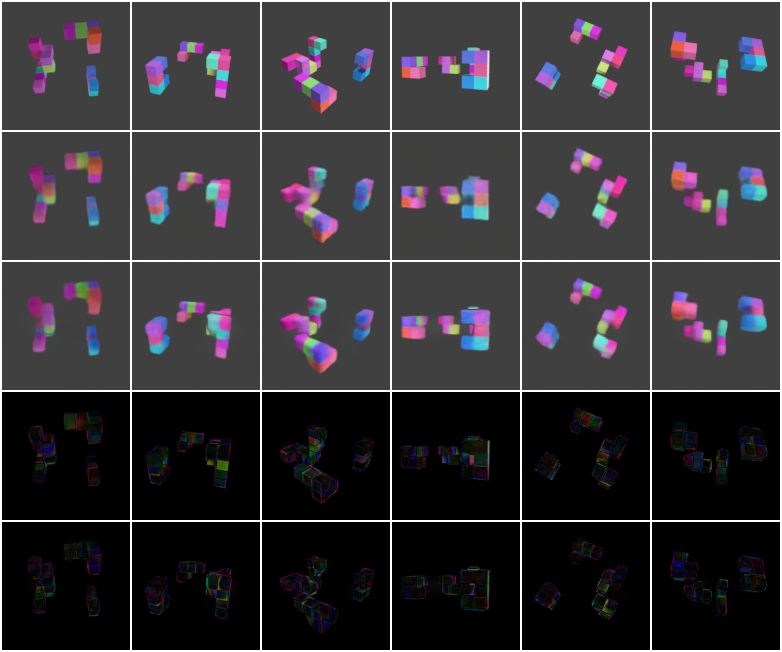
Appendix A. Generation Samples
We provide more generation samples in this section. For each scene in Figure 8, we show 8
sampled context images in the top row, superimposed with predicted bounding boxes. We
also show generations from three query viewpoints, together with the decomposed object-wise
rendering results. Similar visualizations for two scenes from the 3-5 Shapes data set are
provided in Figure 9.

 Context Observations

 Target Generation Decomposition

 Context Observations

 Target Generation Decomposition

 Figure 8: Generation samples from the Multi-Shepard-Metzler data set.

 20

Context Observations

Target Generation Decomposition

 Context Observations

Target Generation Decomposition

 Figure 9: Generation samples from the 3-5 Shapes data set.

 21

Appendix B. Object Models
In this section, we provide two more samples of the learned object models. As shown in
Figure 10, each object model inferred from a multi-object scene can generate complete object
appearance given different query viewpoints.

 Pitch

 Pitch

 Yaw

 Figure 10: Visualization of learned object models from a set of query viewpoints.

 22

Appendix C. Summary of ROOTS Encoder and Decoder

Algorithm 1 ROOTS Encoder
Input: contexts C = {(xc , vc )}K c=1 , partition resolutions Nx , Ny , Nz
Define: [J] = {1, 2, . . . , J} for any natural number J
 1: Obtain Geometric Volume Feature Map r = fctx enc (C)
 2: for each (i, j, k) ∈ [Nx ] × [Ny ] × [Nz ] parallel do
 3: Infer object presence and position in 3D world coordinates: zpres where ∼ f
 ijk , zijk pres,where (r)
 4: end for
 P pres
 5: Obtain the number of objects N = ijk zijk
 pres
 6: Map each (i, j, k) with zijk = 1 to an object index n ∈ [N ]
 7: for each object n ∈ [N ] parallel do
 8: for each context (xc , vc ) ∈ C parallel do
 9: Infer 2D object location owhere n,c using Attention-by-Perspective-Projection
10: Crop 2D object patch xn,c from xc using owhere
 att
 n,c
11: end for
12: Obtain object context Cn = {(xatt where K
 n,c , vc , on,c )}c=1
13: Infer 3D object appearance zn what ∼ GQNenc (Cn )
14: 3D
 Build object model zn = (zn where , zwhat )
 n
15: end for
16: return object models {z3D N
 n }n=1 , object contexts {Cn }n=1
 N

Algorithm 2 ROOTS Decoder
Input: object models {z3D N N M
 n }n=1 , object contexts {Cn }n=1 , query viewpoints vQ = {vq }q=1
Define: [J] = {1, 2, . . . , J} for any natural number J
 1: for each query viewpoint vq ∈ vQ parallel do
 2: for each object n ∈ [N ] parallel do
 3: Obtain object context encoding rnatt = fobj ctx enc (Cn )
 4: Decode 3D appearance into 2D image patch:
 owhat
 n,q = GQNdec (concat[zn
 what , r att ], v )
 n q
 5: Infer 2D object location owhere
 n,q using Attention-by-Perspective-Projection
 6: Obtain image layer x̂n,q and transparency map αn,q from owhat where
 n,q and on,q
 7: end for
 Composite the full image x̂q = N
 P
 8: n=1 αn,q x̂n,q
 9: end for
10: return generations {x̂q }M q=1

 23

Appendix D. Perspective Projection
Following GQN (Eslami et al., 2018), we parameterize the viewpoint v as a tuple (w, y, p),
where w ∈ R3 is the position of the camera in world coordinates, and y ∈ R and p ∈ R are
its yaw and pitch respectively. We also assume access to the intrinsic camera parameters,
including focal length f ∈ R and sensor size, that are the same across all scenes. APPpos
converts the center position of an object n from world coordinates zwhere
 n ∈ R3 to image
 center depth > 3
coordinates [on , on ] ∈ R as follows:
 [a, b, d]> = Ry,p (zwhere
 n − w) , ocenter
 n = normalize([fa/d, fb/d]> ) , odepth
 n =d.
Here, Ry,p is a 3 × 3 rotation matrix computed from the camera yaw and pitch, [a, b, d]>
represents the center position of the object in camera coordinates, and [a, b]> is further
normalized into image coordinates ocenter
 n , using the focal length and sensor size, so that
the upper-left corner of the image corresponds to [−1, −1]> and the lower-right corner
corresponds to [1, 1]> .

Appendix E. Transparency Map
The transparency map αn,q ensures that occlusion among objects is properly handled for
a query viewpoint vq . Ideally, αn,q (i, j) = 1 if, when viewed from vq , the pixel (i, j) is
contained in object n and is not occluded by any other object, and αn,q (i, j) = 0 otherwise.
On the other hand, the object mask m̂n,q is expected to capture the non-occluded full
object, that is, m̂n,q (i, j) = 1 if the pixel (i, j) is contained in object n when viewed from
vq , regardless of whether it is occluded or not. Therefore, we compute αn,q by masking out
occluded pixels from m̂n,q :
 αn,q = wn,q m̂n,q ,
where is pixel-wise multiplication, and wn,q (i, j) = 1 if object n is the closest one to the
camera among all objects that contain the pixel (i, j). In actual implementation, αn,q , m̂n,q ,
and wn,q are not strictly binary, and we obtain the value of wn,q at each pixel (i, j) by the
masked softmax over negative depth values:
 m̂n,q (i, j) exp (−odepth
 n,q )
 wn,q (i, j) = PN depth
 .
 n=1 m̂n,q (i, j) exp (−on,q )

Appendix F. Data Set Details
In this section, we provide details of the two data sets we created.
 Shapes. There are 3 types of objects: cube, sphere, and cylinder, with 6 possible colors
to choose from. Object sizes are sampled uniformly between [0.56, 0.66] units in the MuJoCo
(Todorov et al., 2012) physics world. All objects are placed on the z = 0 plane, with a range
of [−2, 2] along both x-axis and y-axis. We randomly sample 30 cameras for each scene.
They are placed at a distance of 3 from the origin, but do not necessarily point to the origin.
The camera pitch is sampled between [π/7, π/6] so that the camera is always above the
z = 0 plane. The camera yaw is sampled between [−π, π].
 Multi-Shepard-Metzler. We generate the Shepard-Metzler objects as described in
GQN (Eslami et al., 2018). Each object consists of 5 cubes with edge length 0.8. Each cube

 24

is randomly colored, with hue between [0, 1], saturation between [0.75, 1], and value equal
to 1. Like the Shapes data set, all objects are placed on the z = 0 plane, with a range of
[−3, 3] along both x-axis and y-axis. We randomly sample 30 cameras for each scene and
place them at a distance of 12 from the origin. They all point to the origin. The camera
 5 5
pitch is sampled between [− 12 π, 12 π], and the yaw is sampled between [−π, π].

Appendix G. ROOTS Implementation Details
In this section, we introduce the key building blocks for implementing ROOTS.
 Context Encoder. The context encoder is modified based on the ‘tower’ representation
architecture in GQN (Eslami et al., 2018). It encodes each pair of context image and the
corresponding viewpoint into a vector. Summation is applied over the context encodings to
obtain the order-invariant representation ψ.
 Object-Level Context Encoder. The object-level context encoder is also an adapta-
tion of the ‘tower’ representation architecture, but takes the extracted object-level context
Cn as input.
 ConvDRAW. We use ConvDRAW (Gregor et al., 2016) to infer the prior and posterior
distributions of the latent variables. To render the objects and the background, we use a
deterministic version of ConvDRAW (i.e., without sampling). In the following, we describe
one rollout step (denoted l) of ConvDRAW used in ROOTS generative and inference
processes, respectively. We provide detailed configurations of each ConvDRAW module in
Table 6.

 • Generative Process:

 (h(l+1)
 p , c(l+1)
 p ) ← ConvLSTMθ (ψC , z(l) , h(l) (l)
 p , cp )

 z(l+1) ∼ StatisNetθ (h(l+1)
 p )

 • Inference Process:

 (h(l+1)
 p , c(l+1)
 p ) ← ConvLSTMθ (ψC , z(l) , h(l) (l)
 p , cp )

 (h(l+1)
 q , c(l+1)
 q ) ← ConvLSTMφ (ψC , ψQ , h(l) (l) (l)
 p , hq , c q )

 z(l+1) ∼ StatisNetθ (h(l+1)
 q )

Here, ψC and ψQ are order-invariant encodings of contexts and queries respectively, and
z(l+1) is the sampled latent at the (l + 1)-th step. The prior module is denoted by subscript
p, with learnable parameters θ, and the posterior module is denoted by subscript q, with
learnable parameters φ. StatisNet maps hidden states to distribution parameters, and will
be explained in the following. ConvLSTM replaces the fully-connected layers in LSTM
(Hochreiter and Schmidhuber, 1997) by convolutional layers.
 Sufficient Statistic Network. The Sufficient Statistic Network (StatisNet) outputs
sufficient statistics for pre-defined distributions, e.g., µ and σ for Gaussian distributions, and
ρ for Bernoulli distributions. We list the configuration of all Sufficient Statistic Networks
in Table 7. For zwhere
 n , zwhat
 n , and zbg , we use ConvDraw to learn the sufficient statistics.
 pres
For zn , two ConvBlocks are first used to extract features, and then a third ConvBlock

 25

Module Name Rollout Steps Hidden Size
 zbg 2 128
 zwhere 2 128
 zwhat 4 128
 Object Renderer 4 128
 Background Renderer 2 128

 Table 6: Configuration of ConvDRAW modules.

 Object-Level Latent Variables
 zwhere zwhat
 Conv3D(128, 3, 1, GN, CELU) Conv3D(128, 1, 1, GN, CELU)
 Conv3D(64, 1, 1, GN, CELU) Conv3D(64, 1, 1, GN, CELU)
 Conv3D(32, 1, 1, GN, CELU) Conv3D(32, 1, 1, GN, CELU)
 Conv3D(3 × 2, 1, 1, GN, CELU) Conv3D(4 × 2, 1, 1, GN, CELU)
 zpres
 ConvBlock 1 ConvBlock 2 ConvBlock 3
 Conv3D(256, 3, 1, GN, CELU) Conv3D(256, 1, 1, GN, CELU) Conv3D(128, 3, 1, GN, CELU)
 Conv3D(256, 1, 1, GN, CELU) Conv3D(64, 1, 1, GN, CELU)
 Conv3D(1, 1, 1, GN, CELU)
 Scene-Level Latent Variables
 zbg
 Conv3D(1 × 2, 1, 1, GN, CELU)

 Table 7: Configuration of Sufficient Statistic Networks.

combines the features and outputs the parameter of the Bernoulli distribution. GN denotes
group normalization (Wu and He, 2018), and CELU denotes continuously differentiable
exponential linear units (Barron, 2017).

Appendix H. Downstream Task Details
We use the 3-5 Shapes data set for the downstream tasks. To generate the ground-truth
labels, we assign a label to each object based on its type and color. There are 3 different
types and 6 different colors in total, thus the label value for one object lies in the range
from 0 to 17. We split the data set into training set, validation set, and test set of size 50K,
5K, and 5K, respectively. During training, 10 to 20 randomly sampled context observations
are provided for both GQN and ROOTS to learn representations of a 3D scene. All latent
variables are sampled from the learned priors.
 Retrieve Object. To predict the correct class of the object that lies closest to a given
point in the 3D space, the classifier first encodes the scene representation r̂ into a vector, and

 26