Quantitative stratigraphic analysis in a source-to-sink numerical framework
←
→
Page content transcription
If your browser does not render page correctly, please read the page content below
Geosci. Model Dev., 12, 2571–2585, 2019
https://doi.org/10.5194/gmd-12-2571-2019
© Author(s) 2019. This work is distributed under
the Creative Commons Attribution 4.0 License.

Quantitative stratigraphic analysis in a source-to-sink
numerical framework
Xuesong Ding1 , Tristan Salles1 , Nicolas Flament2 , and Patrice Rey1
1 Basin   GENESIS Hub, EarthByte Group, School of Geosciences, The University of Sydney, Sydney, NSW 2006, Australia
2 School   of Earth and Environmental Science, University of Wollongong, Wollongong, NSW 2522, Australia

Correspondence: Xuesong Ding (xuesong.ding@sydney.edu.au)

Received: 25 October 2018 – Discussion started: 28 November 2018
Revised: 21 May 2019 – Accepted: 22 May 2019 – Published: 28 June 2019

Abstract. The sedimentary architecture at continental mar-        automatically produce stratigraphic interpretations. Our re-
gins reflects the interplay between the rate of change of         sults suggest that the analysis of the presented model is more
accommodation creation (δA) and the rate of change of             robust with the accommodation succession method than with
sediment supply (δS). Stratigraphic interpretation increas-       the trajectory analysis method. Stratigraphic analysis based
ingly focuses on understanding the link between deposition        on manually extracted shoreline and shelf-edge trajectory re-
patterns and changes in δA/δS, with an attempt to recon-          quires calibrations of time-dependent processes such as ther-
struct the contributing factors. Here, we use the landscape       mal subsidence or additional constraints from stratal termina-
modelling code pyBadlands to (1) investigate the develop-         tions to obtain reliable interpretations. The 3-D stratigraphic
ment of stratigraphic sequences in a source-to-sink context;      analysis of the presented model reveals small lateral vari-
(2) assess the respective performance of two well-established     ations of sequence formations. Our work provides an effi-
stratigraphic interpretation techniques: the trajectory analy-    cient and flexible quantitative sequence stratigraphic frame-
sis method and the accommodation succession method; and           work to evaluate the main drivers (climate, sea level and tec-
(3) propose quantitative stratigraphic interpretations based      tonics) controlling sedimentary architectures and investigate
on those two techniques. In contrast to most stratigraphic for-   their respective roles in sedimentary basin development.
ward models (SFMs), pyBadlands provides self-consistent
sediment supply to basin margins as it simulates erosion,
sediment transport and deposition in a source-to-sink con-
text. We present a generic case of landscape evolution that       1   Introduction
takes into account periodic sea level variations and passive
margin thermal subsidence over 30 million years, under uni-       Since its introduction in 1970s, sequence stratigraphy has
form rainfall. A set of post-processing tools are provided to     been widely used to interpret depositional architectures in
analyse the predicted stratigraphic architecture. We first re-    terms of variations in eustatic sea level or relative sea level
construct the temporal evolution of the depositional cycles       (i.e. accommodation) (Vail et al., 1977a; Pitman, 1978; Posa-
and identify key stratigraphic surfaces based on observations     mentier et al., 1988; Posamentier and Vail, 1988; Jervey,
of stratal geometries and facies relationships, which we use      1988). With recognition of the role of sediment supply in
for comparison to stratigraphic interpretations. We then ap-      affecting stratal stacking patterns, the rate of change of ac-
ply both the trajectory analysis and the accommodation suc-       commodation creation (δA) versus the rate of change of sed-
cession methods to manually map key stratigraphic surfaces        iment supply (δS) – the δA/δS ratio – has been widely ac-
and define sequence units on the final model output. Finally,     cepted as the main control of sequence formations (Schlager,
we calculate shoreline and shelf-edge trajectories, the tempo-    1993; Muto and Steel, 1997; Catuneanu et al., 2009; Neal
ral evolution of changes in relative sea level (proxy for δA)     and Abreu, 2009; Neal et al., 2016). The δA/δS concept
and sedimentation rate (proxy for δS) at the shoreline, and       offers several advantages compared to conventional strati-
                                                                  graphic models as it directly relates depositional patterns to

Published by Copernicus Publications on behalf of the European Geosciences Union.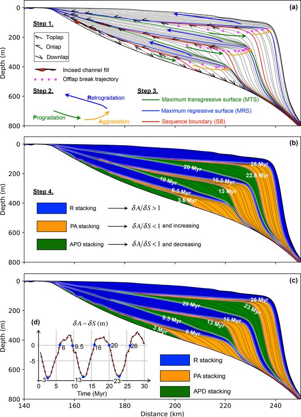
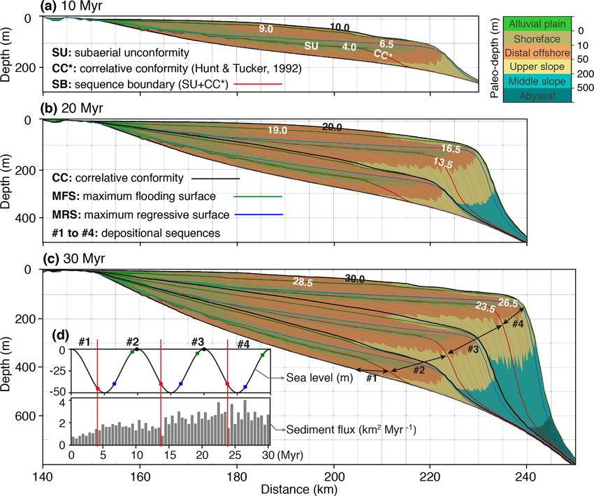
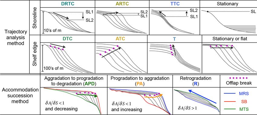
2572                                                        X. Ding et al.: Quantitative stratigraphic analysis in pyBadlands

the main contributing geological drivers (e.g. eustasy, tecton-    Helland-Hansen and Gjelberg (1994), Helland-Hansen and
ics and sediment supply). Yet, the inherent difficulties in ac-    Martinsen (1996), and Helland-Hansen and Hampson (2009)
curately describing accommodation and reconstructing sedi-         proposed the trajectory analysis method that correlates de-
ment supply limit the quantification of the δA/δS ratio and,       positional units with the lateral and vertical migrations of
as a result, the practical application of the δA/δS concept in     the shoreline and shelf-edge trajectories. Neal and Abreu
stratigraphic interpretations (Muto and Steel, 2000; Burgess       (2009) and Neal et al. (2016) proposed a refined sequence
et al., 2016).                                                     stratigraphic framework known as the accommodation suc-
   Experimental stratigraphy (e.g. analogue experiments,           cession method in which sequence sets are interpreted based
stratigraphic forward modelling, SFM) plays a significant          on offlap break trajectory and stratal geometries. The tempo-
role in exploring the development of sedimentary architec-         ral evolution of accommodation change and sediment supply
ture under various forcing conditions (Martin et al., 2009;        can then be derived from interpreted sequence sets and key
Burgess et al., 2012; Muto et al., 2016). Over the past few        stratigraphic bounding surfaces.
decades, SFM has been widely used to investigate the in-              This study also attempts to evaluate the performance of
terplay between major sequence-controlling factors (e.g. eu-       these two approaches to interpret the stratal architecture pre-
stasy, tectonics, flexural isostasy, sediment supply, sediment     dicted with pyBadlands. To illustrate the workflow, we build
compaction, basin physiography) and their influences in the        a synthetic source-to-sink model that includes a mountain
formation of stratigraphic sequences (Reynolds et al., 1991;       range (sediment source), an alluvial plain (sediment transfer
Posamentier and Allen, 1993; Steckler et al., 1993; Carvajal       zone) and a passive continental margin (sink area) where rel-
and Steel, 2009; Burgess et al., 2012; Granjeon et al., 2014;      atively well understood sequence-controlling drivers such as
Csato et al., 2014; Sylvester et al., 2015; Harris et al., 2015,   eustasy and thermal subsidence (Watts and Steckler, 1979;
2016). SFM can therefore provide insights into the quantifi-       Bond et al., 1989; Steckler et al., 1993) are imposed. We
cation of links between sequence formation and the chang-          first present the temporal evolution of predicted stratal stack-
ing δA/δS ratio. Here we use SFM as a tool to investigate          ing patterns and map out key stratigraphic surfaces, which
the development of stratigraphic architecture under the inter-     serves as a reference for comparison to stratigraphic inter-
play between accommodation variations and sediment sup-            pretations. We then follow the trajectory analysis and the ac-
ply. We use the landscape evolution code pyBadlands that           commodation succession method to interpret the predicted
describes sediment transport from source to sink in a self-        stratal architecture. Finally, we design a suite of numeri-
consistent manner (Salles, 2016; Salles and Hardiman, 2016;        cal tools to extract of shoreline and shelf-edge trajectories,
Salles et al., 2018). In pyBadlands, the erosion from up-          as well as accommodation change and sedimentation evolu-
stream catchments is linked to the sedimentation on basin          tion over space and time, with the aim to integrate the tra-
margins through sediment routing resulting from a combi-           jectory analysis method and the accommodation succession
nation of channelling and hillslope processes. As a conse-         method within pyBadlands to derive quantitative interpre-
quence, sediment supply to basin margins is dynamically de-        tations. These new capabilities make it possible to quickly
termined without user control; it results from the interaction     interpret synthetic depositional cycles in a consistent man-
of imposed tectonics, climatic and eustatic variations as well     ner using either the trajectory analysis or the accommodation
as autogenic changes in upstream catchment physiography.           succession method.
   We then apply the rules of sequence stratigraphy to inter-
pret predicted depositional cycles. In sequence stratigraphy,
various sequence models exist and subdivide the stratal suc-       2   Quantitative stratigraphic analysis in pyBadlands
cessions into unconformity- and/or correlated-conformity-
bounded stratigraphic units (Galloway, 1989; Mitchum Jr.,          The workflow to build a quantitative framework of strati-
1977; Van Wagoner et al., 1988; Helland-Hansen and Gjel-           graphic analysis in pyBadlands is illustrated in Fig. 1. In
berg, 1994). These models have been proved to be useful for        this study, we focus on the post-processing of model outputs.
a number of cases. However, the interpretation of systems          pyBadlands records the depth, relative elevation (depth rel-
tracts and sequences based on these sequence models can be         ative to sea level) and thickness of each stratigraphic layer
non-objective and non-unique (Burgess et al., 2016; Burgess        through time. With this information, we are able to extract
and Prince, 2015). Observation-based methods to interpret          cross sections and to reconstruct the temporal evolution of
stratigraphic sequences have the advantage of being objec-         stratal stacking patterns and 3-D Wheeler diagrams at any
tive and independent of spatial and temporal scales. Hence,        location. The 3-D Wheeler diagram contains information of
over the years, it has been recognized that stratigraphic in-      distance along the cross section, time and deposited sediment
terpretations should be guided by physical observations and        thickness. This allows us to identify key stratigraphic sur-
be independent of depositional models and associated as-           faces based on observations of stratal geometry and facies
sumptions (Abreu et al., 2014; Burgess et al., 2016; Neal          relationships.
et al., 2016). Here, we focus on two such methods: the tra-           We then interpret the synthetic depositional cycles in two
jectory analysis and the accommodation succession method.          ways. First, we follow the workflow proposed in the tra-

Geosci. Model Dev., 12, 2571–2585, 2019                                              www.geosci-model-dev.net/12/2571/2019/
X. Ding et al.: Quantitative stratigraphic analysis in pyBadlands                                                                2573

                                                                       the retrogradation stacking (R) for δA/δS > 1, the progra-
                                                                       dation to aggradation stacking (PA) for δA/δS < 1 and in-
                                                                       creasing, and the aggradation to progradation (even to degra-
                                                                       dation) stacking (AP or APD) for δA/δS < 1 and decreas-
                                                                       ing (and possibly negative). The three key surfaces bounding
                                                                       these stacking patterns are the sequence boundary (SB), the
                                                                       maximum transgressive surface (MTS) and the maximum re-
                                                                       gressive surface (MRS).
                                                                          We manually mark the shelf-edge (or offlap break) tra-
                                                                       jectory and stratal terminations on the final output of stratal
                                                                       stacking pattern reconstructed from a simulated cross sec-
                                                                       tion. Key stratigraphic surfaces and stacking patterns are then
                                                                       defined.
                                                                          Second, a series of post-processing tools are implemented
                                                                       in pyBadlands to numerically extract the shoreline and shelf-
                                                                       edge positions, as well as the temporal evolution of δA and
                                                                       δS through time and space (Fig. 3). The shoreline position
                                                                       is recorded by tracking the topographic contour that corre-
                                                                       sponds to sea level. The shelf edge is calculated by assuming
                                                                       a critical slope of 0.025◦ in this case. Changes in relative sea
Figure 1. Workflow to build the stratigraphic architecture in pyBad-   level and sedimentation rate are used as proxies for δA and
lands. We present three different ways of stratigraphic interpreta-    δS (Poag and Sevon, 1989; Galloway and Williams, 1991;
tion. The new post-processing workflows designed to automatically      Liu and Galloway, 1997; Galloway, 2001). Therefore, δA at
interpret stratigraphic sequences are shown in the blue boxes.
                                                                       any given location from time T1 to T2 integrates changes
                                                                       in eustatic sea level and basement subsidence, and δS at
                                                                       any given location between time T1 and T2 is given by de-
jectory analysis and the accommodation succession method               posited strata thickness. In this study, both δA and δS are in
to subdivide the stratigraphic record. The trajectory analy-           m Myr−1 . We then extract δA and δS at shoreline positions
sis technique defines different trajectory classes based on the        through time. Trajectory classes, stacking patterns and strati-
trajectories recorded at either shoreline or shelf-edge posi-          graphic surfaces are defined automatically based on calcu-
tions (Helland-Hansen and Gjelberg, 1994; Helland-Hansen               lated shoreline, shelf-edge trajectories, and time-dependent
and Martinsen, 1996; Helland-Hansen and Hampson, 2009).                δA and δS.
Though both represents a break in slope, the shelf edge
evolves at larger spatial (Fig. 2) and over longer tempo-
ral scales than the shoreline, making it easier to define the          3   Experimental setup
shelf edge on seismic data. By investigating the migration
direction of the shoreline and the shelf edge, four shore-             We provide an example to illustrate how our workflow can be
line trajectory classes and three shelf-edge trajectory classes        used to automatically generate stratigraphic sequences and
are used to characterize the successive depositional pack-             analyse them in an integrated numerical toolbox.
ages. The shoreline trajectory classes include the transgres-             We create an initial synthetic landscape of dimensions
sive trajectory class (TTC), the ascending regressive trajec-          300 km by 200 km with a spatial resolution of 0.5 km. The
tory class (ARTC), the descending regressive trajectory class          region includes a mountain range, an alluvial plain and an
(DRTC) and the stationary (i.e. non-migratory) shoreline tra-          adjacent continental margin consisting of a continental shelf,
jectory class. The shelf-edge trajectory classes include de-           a continental slope and an oceanic basin. Details of the
scending trajectory class (DTC), ascending trajectory class            geometry are presented in Fig. 4a. The model duration is
(ATC), transgressive trajectory class (T) and stationary or flat       30 Myr, generating 300 stratigraphic layers with display in-
trajectory class (Fig. 2).                                             tervals every 0.1 Myr. Our model setting mimics the first-
   Neal and Abreu (2009) and Neal et al. (2016) presented a            order, long-term landscape evolution and associated strati-
refined hierarchy framework, known as the accommodation                graphic sequence development along a passive continental
succession method, in which the subdivision of depositional            margin, with forcing conditions including climate, eustatic
units is entirely based on the stratal geometry resulting from         sea level change and thermal subsidence.
the evolution of accommodation change and sediment infill.                In this study, we use a single flow direction, detachment-
Three stacking patterns and their bounding surfaces are de-            limited stream power law, and a simple downslope creep
fined and subsequently used to assess the changing history of          law to describe erosion, sediment transport and deposition.
accommodation and sediment supply (Fig. 2). These include              Equations and model parameters are provided in the Supple-

www.geosci-model-dev.net/12/2571/2019/                                                   Geosci. Model Dev., 12, 2571–2585, 2019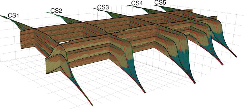
2574                                                             X. Ding et al.: Quantitative stratigraphic analysis in pyBadlands

Figure 2. Stratigraphic sequence interpretation approaches used in this study. In the trajectory analysis method, four shoreline trajectory
classes and three shelf-edge trajectory classes are delineated based on the lateral and vertical migrations of shoreline and shelf edge. The
shoreline trajectory classes include descending regressive trajectory class (DRTC), ascending regressive trajectory class (ARTC), transgres-
sive trajectory class (TTC) and stationary trajectory class. The shelf-edge trajectory classes include descending (DTC), ascending (ATC),
transgressive (T) and stationary shelf-edge trajectory classes (Helland-Hansen and Gjelberg, 1994; Helland-Hansen and Martinsen, 1996;
Helland-Hansen and Hampson, 2009). In the accommodation succession method, three types of stacking patterns and their bounding surfaces
are defined based on observations of stratal terminations (e.g. onlap, offlap) and stratal geometries, including aggradation to progradation to
degradation (APD) stacking, progradation to aggradation (PA) stacking and retrogradation (R) stacking. The bounding surfaces are sequence
boundary (SB), maximum transgressive surface (MTS) and maximum regressive surface (MRS). Each stacking pattern reflects changes in
the rate of accommodation creation (δA) with respect to the rate of sediment supply (δS) at the shoreline. APD stacking corresponds to
δA/δS < 1, with a decreasing trend that can be negative; PA stacking represents δA/δS < 1 and increasing; finally, R stacking occurs for
δA/δS > 1 (Neal and Abreu, 2009; Neal et al., 2016).

ment. Considering that this study focuses on long-term strati-            is
graphic evolution due to sea level change, both climate and
subsidence patterns are considered constant. Climate is as-               S(t) = E0 r − E0 exp(−t/τ ),                                     (1)
sumed to be directly related to precipitation with a spatially
and temporally uniform precipitation rate of 2.0 m yr−1 over              where E0 = 4aρ0 αT1 /π 2 (ρ0 − ρw ), r = πβ sin( πβ ), a =
30 Myr. The sediment input varies through time, depending                 125 km is the thickness of lithosphere, ρ0 = 3300 kg m−3 the
on the dynamic evolution of source area.                                  density of the mantle at 0 ◦ C, ρw = 1000 kg m−3 the density
   Sea level fluctuations are a major driver of changes in ac-            of seawater, α = 3.28 × 10⁻⁵ K−1 the thermal expansion
commodation and thus stratigraphic sequence development.                  coefficient for both the mantle and the crust, T1 = 1333 ◦ C
They act at different temporal scales, resulting in various               the temperature of the asthenosphere and τ = 62.8 Myr the
stratigraphic cycles with first-order cycles of duration around           characteristic thermal diffusion time. The stretching factor
200–300 Myr, second-order cycles of duration around 10–                   β characterizes the extension of the lithosphere. These
80 Myr and third-order cycles of duration around 1–10 Myr                 parameters are taken from McKenzie (1978). In our exper-
(Vail et al., 1977b). Here we consider the effects of long-               iments, thermal subsidence is imposed on the continental
term eustatic cycles and assume that eustasy is independent               margin, starting from the initial shoreline (Fig. 4a), which
of climate and local tectonics. For simplicity, eustatic sea              experiences the least subsidence, to the outward edge where
level is modelled using a sinusoidal curve consisting of three            subsidence is maximum. We take β as distance-dependent
10 Myr cycles of 50 m amplitude (Fig. 4b), which correspond               and calculate the thermal subsidence accumulated at 10,
to second- to third-order eustatic fluctuations (Vail et al.,             20 and 30 Myr, respectively (Fig. 4c). The subsidence rate
1977b).                                                                   is constant at each single position but increases along the
   Thermal subsidence is an important process leading to                  x axis. In our model, relative sea level is the combined result
the deepening of the basin floor due to isostatic adjustment              of eustatic sea level and thermal subsidence and thus varies
during lithosphere cooling. A simple stretching model from                spatially due to basement subsidence.
McKenzie (1978) is applied in this study, in which subsi-
dence is produced by thermal relaxation following an episode
of extension. The equation to derive the subsidence at time t

Geosci. Model Dev., 12, 2571–2585, 2019                                                      www.geosci-model-dev.net/12/2571/2019/
X. Ding et al.: Quantitative stratigraphic analysis in pyBadlands 2575
clinoform develops due to the falling eustatic sea level, with
strata toplapped by a subaerial unconformity (SU). This sub-
aerial unconformity terminates downdip at the offlap-break
at 4.0 Myr and it transfers to a marine correlative conformity
(CC∗ ), which together forms a sequence boundary (Fig. 5a).
The shoreline steps back and strata onlap the subaerial un-
conformity from 4.0 Myr. The prograding packages then shift
to aggradational pattern until 6.5 Myr when the shelf edge
reaches its most basinward location, marked by the maxi-
mum regressive surface at 6.5 Myr. Eustatic sea level first
falls and then rises at a relative slow changing rate between
4.0 and 6.5 Myr, and the clinoform formed during this period
is characterized by thin topsets and thick foresets. The sed-
iment flux constantly increases from 0.7 to 2.0 km2 Myr−1
over the first 6.5 Myr (Fig. 5d), with small variations due to
the lateral shifts in the position of the river mouth. Eustatic
sea level rises from 6.5 to 9.0 Myr, and strata continue on-
lapping the subaerial unconformity and fill incised channels
with fluvial sediments to form a maximum flooding surface
(MFS) at 9.0 Myr. The clinoform formed during this time
period is characterized by thick topsets and an absence of
foresets. From 9.0 to 10.0 Myr, the shoreline steps back and
strata continue onlapping while the stacking pattern changes
Figure 3. Schematic diagram showing the sedimentation from
from retrogradation to aggradation. During the phase of sea
time 1 (T1) to time 2 (T2) under sea level variation and basement
subsidence. The depth, relative elevation and thickness of strati- level rise from 6.5 to 10.0 Myr, the sediment flux slightly de-
graphic layer are recorded at every time step (dT = T2 − T1). Post- creases to 1.6 km2 Myr−1 (Fig. 5d). Eustatic sea level falls
processing tools extract the shoreline and shelf-edge positions and from 10 to 13.5 Myr and strata stacking changes to progra-
calculate the rate of accommodation creation (δA) and the rate of dation, forming a second subaerial unconformity (Fig. 5b).
sedimentation (δS) through time. The shoreline position is recorded The surface formed at 10.0 Myr that separates aggradation
by tracing the topographic contour that corresponds to sea level. from progradation is defined as correlative conformity (CC).
The shelf edge is calculated by assuming a critical slope 0.025◦ . δA Mid-slope sediments start to accumulate within the progra-
is calculated as changes in relative sea level at shoreline position dational clinoform between 10.0 and 13.5 Myr. The sediment
over (T2 − T1): (sea level change + subsidence) / (T2 − T1); δS is flux from 10.0 to 13.5 Myr reveals a gentle increasing trend
calculated as deposited strata thickness at shoreline position over
with large variations of up to 0.8 km2 Myr−1 , followed by a
(T2 − T1): (strata thickness) / (T2 − T1).
significant drop in sediment flux at 13.5 Myr (Fig. 5d). The
stratigraphic units accumulated between 4.0 and 13.5 Myr
4 Results form a complete sequence (no. 2) bounded by two composite
surfaces consisting of subaerial unconformities and correla-
4.1 Temporal evolution of stratal architecture tive conformities.
Following the same criteria for identification of strati-
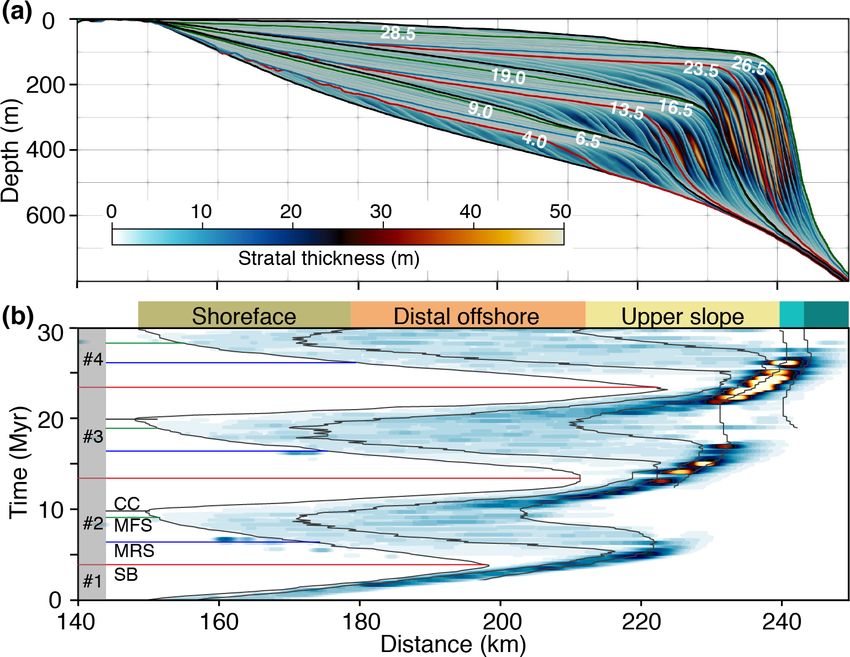
Our post-processing tools quickly extract simulated stratal graphic surfaces, a complete sequence (no. 3) is defined
stacking patterns as well as Wheeler diagrams in any re- from 13.5 to 23.5 Myr, with the maximum regressive surface
gion of the simulated domain. Figure 5 presents the devel- formed at 16.5 Myr, the maximum flooding surface formed at
opment of stratal stacking pattern generated along a dip- 19.0 Myr and the correlative conformity formed at 20.0 Myr
oriented cross section through the middle of the domain. The (Fig. 5b and c). The sediment flux from 13.5 to 23.5 Myr
stratal architecture is coloured based on depositional envi- shows an increasing trend with large variations of up to
ronments defined using six paleo-depth windows. We infer 1.1 km2 Myr−1 , followed by a significantly drop from 2.8 to
depositional facies, changes in depositional trends, stratal ter- 1.5 km2 Myr−1 at 23.5 Myr (Fig. 5d). From 23.5 to 30 Myr,
minations and stratal geometries from the temporal evolution an incomplete sequence (no. 4) develops with a maximum
of stratal stacking patterns. This information is then used to regressive surface at 26.5 Myr and a maximum flooding sur-
identify stratigraphic surfaces and to define systems tracts face at 28.5 Myr. The sediment flux during this time period
and sequences (Van Wagoner et al., 1988). Sediment flux is shows two anomalous peaks at 24.0 and 26.5 Myr (Fig. 5d).
extracted along the cross section by computing the total vol- We also reconstructed the final stratal stacking pattern by
ume of deposited sediments per unit width in 0.5 Myr inter- computing stratal thickness in 100 kyr increments (Fig. 6a),
vals (Fig. 5d). As shown in Fig. 5a, an oblique prograding which constitutes the basis for a 3-D Wheeler diagram
www.geosci-model-dev.net/12/2571/2019/ Geosci. Model Dev., 12, 2571–2585, 2019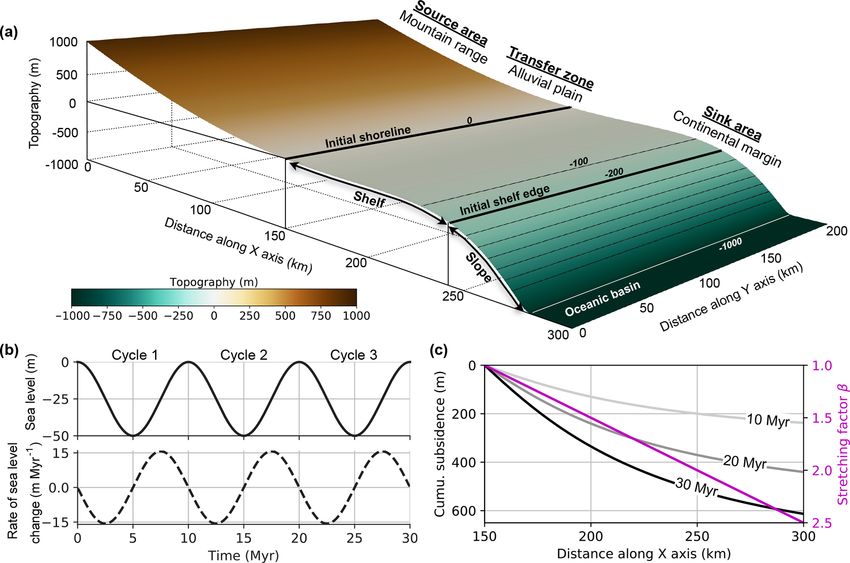
2576                                                            X. Ding et al.: Quantitative stratigraphic analysis in pyBadlands

Figure 4. Model setup. (a) The initial surface elevation of the mountain region ranges from 200 to 1000 m over a width of 100 km, while
the elevation of the alluvial plain ranges from 0 to 200 m over a width of 50 km. The sink area includes a continental margin in which the
elevation of the continental shelf ranges from −250 to 0 m over a width of 80 km, the elevation of the continental slope ranges from −1000
to −250 m over a width of 40 km and a flat oceanic basin whose depth is −1000 m over a width of 30 km. Black lines are isobaths with
an interval of 100 m. The initial elevations of shoreline and shelf edge are 0 and −200 m. (b) Eustatic sea level and its rate of change over
30 Myr. The eustatic sea level scenario modelled using a sinusoidal curve consisting of three 10 Myr cycles of 50 m peak-to-peak amplitude.
(c) Distance-dependent stretching factor β and the resulting thermal subsidence at 10, 20 and 30 Myr across the continental margin.

(Fig. 6b). The 3-D Wheeler diagram shows the horizon-                    the timing of maximum regressive surface agrees well with
tal distribution of depositional environments and the accu-              the onset of decreasing stratal thickness. Sequence bound-
mulated sediment thickness along the cross section through               aries correspond to the shift of shoreline from forestepping
time. Deposition hiatuses and condensed sections, which are              to backstepping, while correlative conformities correspond
essential to recognize bounding surfaces such as subaerial               to the shift of shoreline from backstepping to forestepping.
unconformities or sequence boundaries, are also denoted on
the Wheeler diagram, as well as transgressive and flooding               4.2     Interpretation of depositional sequences
surfaces (Payton et al., 1977; Miall, 2004). The stratal thick-
ness pattern shows three cycles, with thicker sediment ac-               We now focus on the interpretation of the stratal architecture
cumulation during progradational and aggradational stratal               using both the trajectory analysis and accommodation suc-
stacking accompanied with a low rate of eustatic sea level               cession methods.
change, and thinner sediment accumulation during retrogra-
dational stratal stacking accompanied with rising eustatic sea           4.2.1    Trajectory analysis
level. The stacking of sequences no. 1 to no. 4 shows an
aggradational progradation pattern, with at least 10 km sea-             On the stratal stacking pattern extracted from the final output
ward progradation between successive cycles. Eustatic sea                at 30 Myr, we manually pick the break in slope of the shelf-
level fluctuations control sequence formations, as expected,             slope-scale clinoforms as shelf-edge positions (magenta dots
and the effect of thermal subsidence and offshore sedimenta-             in Fig. 7a). Shoreline positions are difficult to pick on the
tion can be recognized when taking the stratigraphic pack-               cross section because shoreline clinoforms are not well de-
age as a whole: the aggradational stacking reveals contri-               veloped with this model setting. We therefore focus on the
butions of basement subsidence in creating accommodation,                analysis of shelf-edge trajectory evolution. According to lat-
while the progradational stacking reveals the contributions of           eral and vertical shifts of the shelf edge through time, de-
offshore sedimentation in decreasing accommodation. When                 scending shelf-edge trajectory classes are identified from 0 to
correlating the formation of stratigraphic surfaces with the             5, 10 to 14, and 20 to 23 Myr; ascending shelf-edge trajectory
horizontal migration of depositional packages, we find that              classes are recognized from 5 to 6.5, 14 to 17, and from 23 to

Geosci. Model Dev., 12, 2571–2585, 2019                                                     www.geosci-model-dev.net/12/2571/2019/
X. Ding et al.: Quantitative stratigraphic analysis in pyBadlands                                                                            2577

Figure 5. Temporal evolution of stratal stacking patterns at 10 Myr (a), at 20 Myr (b) and at 30 Myr (c). Light-grey solid lines represent
timelines at 0.5 Myr intervals. Coloured solid lines with timing in millions of years (Myr) are identified stratigraphic surfaces. Stratal stacking
patterns are coloured by paleo-depth used to represent different depositional environments. Four sequences, no. 1 to no. 4, are defined.
(d) Inset in (c): eustatic sea level curve and its rate of change. Coloured dots indicate the timing of corresponding stratigraphic surfaces. The
paleo-depth and topography shown in this figure are directly produced by our post-processing tool.

26.5 Myr; and transgressive shelf-edge trajectory classes are               detected lateral and vertical migrations of the shoreline posi-
defined from 6.5 to 10, 17 to 20, and 26.5 to 30 Myr (Fig. 7a).             tion and interpreted shoreline trajectory classes accordingly.
   In addition to manually picking the shelf-edge trajectory                The descending regressive trajectory class is identified from
on the final output, we developed post-processing tools to ex-              0 to 4, 10 to 13.5, and 20 to 23 Myr; the transgressive trajec-
tract time-dependent shelf-edge and shoreline positions from                tory class is identified from 5 and 10, 15 and 20, and 25 to
successive outputs and interpret predicted depositional cy-                 30 Myr (Fig. 7c). DRTC and TTC are separated by an ero-
cles accordingly. Figure 7b displays the extracted lateral and              sional surface and a depositional hiatus, whereas the tran-
vertical migrations of the shelf-edge position and interpreted              sition from TTC to DRTC is related to condensed stacking
shelf-edge trajectory classes. The descending shelf-edge tra-               sections in the distal area induced by limited sediment sup-
jectory class is identified from 0 to 5.5, 10 to 13, and 20 to              ply (Fig. 5c). We note that between 4 and 5, 13.5 and 15, and
22.5 Myr; the ascending shelf-edge trajectory class is identi-              23 and 25 Myr, the shoreline migrates landward even though
fied from 5.5 to 6.5, 13 to 16.5, and from 22.5 to 25.5 Myr;                sea level is falling – we call this trajectory type the “descend-
and the transgressive shelf-edge trajectory class is identified             ing transgressive trajectory class” (DTTC) as this shoreline
from 6.5 to 10, 16.5 to 20, and 25.5 to 30 Myr (Fig. 7b).                   evolution is not described in the literature. In our models,
The shelf-edge trajectory classes identified through time gen-              the DTTC occurs because the basement subsidence overrides
erally resemble the ones identified manually from the final                 the falling sea level and thus creates positive accommoda-
output, with differences in the timing of transition from one               tion (Fig. 7e). This phenomenon is due to the model forcing
class to another by up to 1.5 Myr, which is greater than the                conditions, and its identification directly linked to the time-
temporal resolution (0.5 Myr) used to represent stratigraphic               dependent analysis of shoreline trajectory carried out here.
sequences (Fig. 7a and b).
   We now use the post-processing toolbox to identify                       4.2.2    Accommodation succession analysis
changes in shoreline trajectories that are difficult to pick
manually for this case. Figure 7c displays the automatically                Next, we apply the accommodation succession method to
                                                                            analyse the sequence formation in terms of changes in ac-

www.geosci-model-dev.net/12/2571/2019/                                                          Geosci. Model Dev., 12, 2571–2585, 2019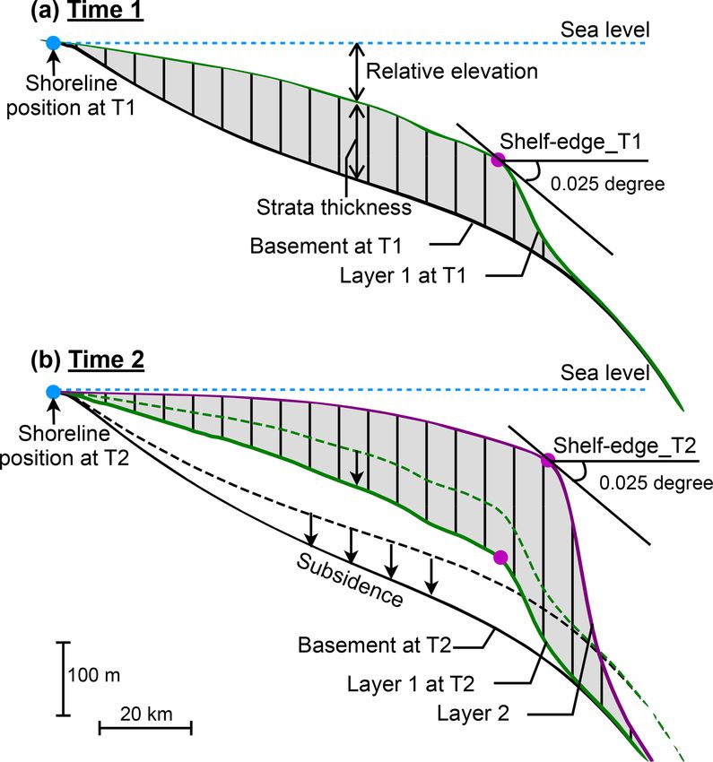
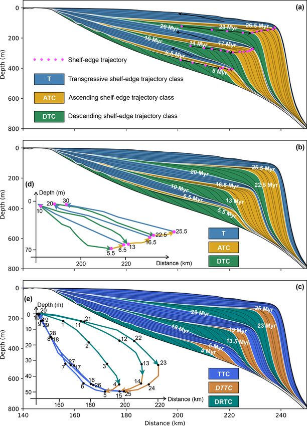
2578                                                          X. Ding et al.: Quantitative stratigraphic analysis in pyBadlands

Figure 6. (a) Reconstructed stratal stacking pattern at 30 Myr showing the stratal thickness at 0.5 Myr intervals. (b) The 3-D Wheeler
diagram or chronostratigraphy chart showing the horizontal distribution of depositional environments bounded by black solid lines and the
accumulated sediment thickness through time along the extracted cross section.

commodation and sedimentation. Following the workflow                  and is characterized by the formation of thicker clinoform
proposed by Neal et al. (2016), we first manually marked               fronts. This stacking corresponds to the AP class (aggrada-
stratal terminations (i.e. onlap, downlap, toplap) and offlap          tion to progradation). Maximum transgressive surfaces sep-
breaks on the simulated stratal stacking pattern (Step 1 in            arate R stacking from AP stacking. At 13 Myr, onlap termi-
Fig. 8a). Here, the offlap break is defined as the shelf edge          nations are visible and the offlap break starts migrating up-
rather than the shoreline as shoreline-scale clinoforms do not         ward, corresponding to the transition towards PA stacking
develop with these model settings. Three stacking patterns             just above the SB surface. Following the same criteria, suc-
and their bounding surfaces are then defined (Steps 2 and 3 in         cessive stacking of PA, R and AP as well as bounding sur-
Fig. 8a). For example, toplaps and downlaps are observed in            faces (SB, MTS and MRS) are defined on the cross section
the first 3.5 Myr and correspond to progradational (P) stack-          (Fig. 8b). Finally, the interpreted R, AP and PA stacking pat-
ing. The stratal geometry associated with P stacking is char-          terns are used to assess the changing history of δA and δS
acterized by either erosion or by a lack of topset deposi-             (Step 4 in Fig. 8b).
tion and relatively thick clinoform front. Though strata keep             Instead of calculating δA/δS as a ratio (Neal et al., 2016),
downlapping, onlap terminations start replacing toplap ter-            we compute δA − δS at the shoreline over time (Fig. 8d), be-
minations after 3.5 Myr, which reflects successive phases of           cause δS can be equal to zero (Fig. 3). Under this approach,
progradation and aggradation. This depositional trend is de-           δA − δS > 0 corresponds to R stacking and is equivalent to
fined as progradation to aggradation stacking, which is char-          δA/δS > 1; δA−δS < 0 and decreasing corresponds to APD
acterized by thin topset deposits and thick clinoform fronts.          stacking and is equivalent to δA/δS < 1 and decreasing; and
The unconformity formed between P and PA stacking is in-               δA − δS < 0 and increasing corresponds to PA stacking and
terpreted as a sequence boundary. Retrogradation stacking              is equivalent to δA/δS < 1 and increasing. The stacking pat-
corresponds to the onlapping of stratal deposits and landward          terns can then be defined automatically (Fig. 8c) and are al-
shift of offlap break around 6.5 Myr. The thick topset deposit         most identical to the manually identified ones: differences
and condensed distal stacking characterize the stratal geome-          in the timing of the change in stacking pattern are 0.5 Myr
try deposited during this stage. Maximum regressive surfaces           at most, which is equal to the temporal resolution (0.5 Myr)
are defined at the transition between PA and R stacking. At            with which stratigraphic sequences are represented in Figs. 7
10 Myr, the offlap break starts migrating seaward and down-            and 8.
ward. Toplap and downlap terminations are also observed af-
ter this time. The geometry of deposited strata also changes

Geosci. Model Dev., 12, 2571–2585, 2019                                                  www.geosci-model-dev.net/12/2571/2019/
X. Ding et al.: Quantitative stratigraphic analysis in pyBadlands 2579
Figure 7. Interpretation of trajectory classes based on analysis of shoreline and shelf-edge trajectories (Helland-Hansen and Hampson,
2009). (a) Shelf-edge trajectory classes based on manually picking the shelf-edge trajectory (magenta dots) on the final output of stratal
stacking pattern. (b) Automatically picking shelf-edge trajectory classes based on calculated time-dependent shelf-edge positions in (d). (c)
Automatically defined shoreline trajectory classes based on calculated time-dependent shoreline positions in (e). Time labels indicate the
timing of each trajectory class formation. See Fig. 2 for abbreviations.
5 Discussion The manual application of shelf-edge trajectory analysis
presents reliable interpretations of transgressive stratigraphic
units (T) but displays notable discrepancies in separating
We compare and contrast the interpretations resulting descending stratigraphic units (DTC) from ascending strati-
from observations of temporal evolving stratal architecture graphic units (ATC) especially during in the early stages of
(Sect. 4.1) with the interpretations resulting from the manual deposition (Fig. 7a). Note that here we only discuss discrep-
application of both trajectory analysis and accommodation ancies beyond 0.5 Myr, which is the time interval of recon-
succession methods (Sect. 4.2.1) and from quantitative anal- structing stratal stacking patterns in Sect. 4.2. The imposed
ysis of these two methods using our post-processing tools thermal subsidence modifies the position of the shelf-edge
(Sect. 4.2.2).
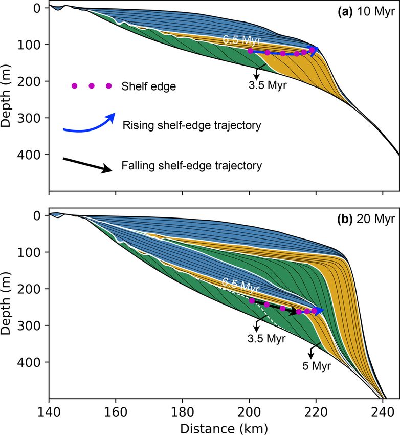
www.geosci-model-dev.net/12/2571/2019/ Geosci. Model Dev., 12, 2571–2585, 20192580 X. Ding et al.: Quantitative stratigraphic analysis in pyBadlands Figure 8. (a–b) Interpretation workflow based on the accommodation succession method (Neal et al., 2016). Step 1 includes marking stratal terminations (i.e. toplap, onlap and downlap represented using small arrows) and manually picking the break in slope as offlap break. The refilling of incised channels is shown in red, indicating erosional surfaces. Based on the marked stratal contacts, three stratal stacking trends (solid arrows) and three stratigraphic surfaces (coloured solid lines) are then defined in Steps 2 and 3. The three interpreted stacking patterns are filled with different colours, with their bounding times marked (Step 4). Each stacking pattern reflects the evolving ratio between rate of accommodation creation (δA) and rate of sediment supply (δS). (c) Automatically defined stacking patterns according to the calculated temporal evolution of δA − δS (> 0, < 0 and decreasing, or < 0 and increasing) (d). positions after its formation (Fig. 9): the shelf-edge trajec- and 9b). This should be kept in mind when identifying shelf- tory appears to rise between 3.5 and 6.5 Myr on the snapshot edge trajectories on seismic profiles, which are by nature at 10 Myr (Fig. 9a), whereas it appears to fall between 3.5 a snapshot of the evolution of a basin. Constraining time- and 5 Myr on the snapshot at 20 Myr (Fig. 9b), because of dependent processes such as thermal subsidence from sedi- ongoing thermal subsidence between 10 and 20 Myr. As a mentary packages would be useful to correct shoreline and consequence, identifying strata on the final output artificially shelf-edge trajectories for these processes. extends the duration of descending trajectory class (Figs. 7a Geosci. Model Dev., 12, 2571–2585, 2019 www.geosci-model-dev.net/12/2571/2019/
X. Ding et al.: Quantitative stratigraphic analysis in pyBadlands                                                              2581

                                                                        The quantitative accommodation succession analysis also
                                                                     shows largely consistent interpretations (Figs. 8c and 5), ex-
                                                                     cept for a 1 Myr discrepancy in demarcating aggradation
                                                                     to progradation to degradation stacking and progradation to
                                                                     aggradation stacking at 3 Myr. We find that the δA−δS curve
                                                                     (Fig. 8d) presents trends similar to the rate of eustatic sea
                                                                     level change (Fig. 4b). This suggests that the evolution of
                                                                     δA − δS is a proxy for the derivative of sea level change
                                                                     with respect to time rather than a direct proxy for sea level
                                                                     change. However, a difference exists between the δA − δS
                                                                     curve and the rate-of-sea-level-change curve: the δA − δS
                                                                     curve shows asymmetrical fluctuations with larger amplitude
                                                                     below zero than above zero, which is attributed to the sed-
                                                                     iment supply. Discrepancies of < 0.5 Myr are observed be-
                                                                     tween the δA − δS curve and the rate of eustatic sea level
                                                                     change curve, which are likely to be related to the temporal
                                                                     resolution (0.5 Myr) used to compute δA − δS.
                                                                        A common issue when calculating the ratio δA/δS is the
                                                                     lack of unique approaches and common dimensional units
                                                                     to define these two metrics (Muto and Steel, 2000; Burgess,
                                                                     2016). Both metrics represent changes in volume over a spe-
Figure 9. Stratal stacking pattern extracted at 10 Myr (a) and       cific time interval and thus should be defined in cubic me-
20 Myr (b). Between 3.5 and 5 Myr, the shelf-edge trajectory         tres per year (m3 yr−1 ). However, difficulties in delineating
changes from rising at 10 Myr to falling at 20 Myr, as a result of   the potential space for sediment deposition require the use
basement subsidence. The descending trajectory class thus extends    of proxies to quantify accommodation. Although the sedi-
to 5 Myr.                                                            mentation rate is often used as a proxy for δS (Poag and
                                                                     Sevon, 1989; Galloway and Williams, 1991; Liu and Gal-
                                                                     loway, 1997; Galloway, 2001), it only provides information
                                                                     about the deposition at a single location and does not reflect
   The quantitative shelf-edge trajectory analysis reveals dis-      the spatial distribution of sedimentation (Petter et al., 2013).
crepancies in defining ascending trajectory classes at 5.5,          Furthermore, the distribution of sediment deposition is not
22.5 and 25.5 Myr (Fig. 7b), as extracting the position of the       determined solely by sediment supply but is a combined
shelf edge is more uncertain for steep strata. The tool we have      result of the distance to sediment source, basin physiogra-
developed can be applied to actual sections as long as seis-         phy and sediment transport efficiency (Posamentier et al.,
mic timelines are accessible. Again, we emphasize that addi-         1992; Posamentier and Allen, 1993). Recently, new meth-
tional constraints from observation of stratal geometry would        ods have been proposed to improve the quantification of δS.
improve the interpretations of stratigraphic units. In terms of      Petter et al. (2013) proposed an approach that directly re-
quantitative shoreline trajectory analysis, the distinction be-      constructs sediment paleo-fluxes from stratigraphic records.
tween the descending transgressive trajectory class and the          Ainsworth et al. (2018) used a technique termed “TSF anal-
transgressive trajectory class is controlled by the eustatic sea     ysis” in which parasequence thickness (T ) is used as proxy
level fluctuations (Fig. 7c). Since the shoreline and the shelf      for accommodation at the time of deposition while parase-
edge represent the break in slope of clinoforms at different         quence sandstone fraction (SF) is used as proxy for sediment
scales (Patruno et al., 2015, Fig. 2), it is not appropriate to      supply. Our work could be used to integrate and test these
apply shoreline trajectory analysis to shelf-slope clinoforms.       new quantitative interpretations based on the evolution of ac-
However, the numerical tools we provided to extract time-            commodation and sedimentation in a stratigraphic modelling
dependent shoreline positions based on a given sea level forc-       framework. The quantification of δA and δS presented here
ing would also be useful and applicable to short-term numer-         could be extended in future work to investigate the interplay
ical and analogue experiments (Martin et al., 2009; Granjeon         between accommodation change and sediment supply in 3-
et al., 2014).                                                       D.
   The stratigraphic interpretations from the accommodation             Our source-to-sink numerical scheme generates 3-D land-
succession method indicate that there is no significant differ-      scape evolution and stratigraphic development, though only
ence between analysing the final output and time-dependent           2-D stratigraphic architectures are extracted along dip-
outputs (Figs. 8b and 5). Therefore, the analysis of the pre-        oriented cross sections. To evaluate the lateral variations in
sented model is more robust with the accommodation suc-              sequence formation potentially induced by sediment diffu-
cession method than with the trajectory analysis method.             sion in offshore environment and lateral migrations of river

www.geosci-model-dev.net/12/2571/2019/                                                 Geosci. Model Dev., 12, 2571–2585, 2019
2582 X. Ding et al.: Quantitative stratigraphic analysis in pyBadlands
Figure 10. Stratal stacking patterns on five dip-oriented cross sections (CS1 to CS5) and two along-strike cross sections. Key stratigraphic
surfaces on CS1 to CS5 are identified and coloured accordingly.
Table 1. Timing of stratigraphic surfaces on CS1 to CS5 (Myr).
No. 1 No. 2 No. 3 No. 4
SB1 MRS1 MRFS1 CC1 SB2 MRS2 MFS2 CC2 SB3 MRS3 MFS3
CS1 3.5 6.5 9.0 10.0 13.0 16.5 18.5 20.0 23.5 26.5 28.5
CS2 3.5 6.5 8.5 10.0 12.0 17.0 19.0 20.0 23.0 26.5 28.0
CS3 3.5 6.5 9.0 10.0 13.5 16.5 19.0 20.0 23.5 26.5 28.5
CS4 3.5 6.5 9.0 10.0 13.5 17.0 18.5 20.0 23.0 26.5 28.5
CS5 3.0 5.5 9.0 10.0 13.0 17.0 19.0 20.0 23.0 27.0 28.0
mouth, we extract five dip-oriented cross sections (CS1 to stratigraphic record. In our framework, sediment transport
CS5) that are parallel to each other and two along-strike cross and supply to the margin is dynamically related to autogenic
sections (Fig. 10). Cross section CS3 is the same one as pre- and allogenic processes. As an example, though forced with
sented in the result section. The timing of key stratigraphic uniform rainfall pattern in the source region, the rate of sed-
surfaces on CS1 to CS5 is shown in Table 1, with differences iment supply to the sink area fluctuates with time (Fig. S1 in
varying from 0.5 to 1.5 Myr. The timing of sequence bound- the Supplement). This highlights the complex relationships
aries shows the most variations, compared to other strati- between erosional signals and the preservation of a deposi-
graphic surfaces. The timings of correlative conformities of tional record (Van Heijst et al., 2001; Kim et al., 2006; Kim,
sequence no. 2 (CC1) and sequence no. 3 (CC2) are consis- 2009). The source-to-sink numerical scheme used in pyBad-
tent on cross sections CS1 to CS5 and correspond to the onset lands makes it possible to explore important questions for
of eustatic sea level fall. The stacking of depositional envi- the future of sequence stratigraphy, such as the role of sedi-
ronments along strike shows increasing variations towards ment supply variations in the generation of stratigraphic se-
the basin. For the presented case there is overall little varia- quences at different temporal scales (Burgess, 2016), as well
tion in stratigraphic sequences across strike and along strike, as the importance of allogenic and autogenic processes in the
which is expected from the model setup. The presented tools formation and evolution of stratal record (Paola, 2000; Paola
can be used for the 3-D stratigraphic analysis of more com- et al., 2009).
plex cases. We modelled the formation of stratigraphic sequences over
We have explored stratigraphic development in a source- 30 Myr, which represents second- to third-order stratigraphic
to-sink context in which the dynamic sediment supply to cycles (Vail et al., 1977b). Over this temporal scale, long-
the passive continental margin depends on climatic and tec- term eustatic sea level changes and dynamic uplift or sub-
tonic evolution in the source area. Therefore, the physio- sidence induced by tectonics or deep-Earth processes (e.g.
graphic evolution of the upstream region controls the deposi- mantle flow-driven dynamic topography) might drive de-
tional patterns in the sink area together with accommodation position (Burgess and Gurnis, 1995; Burgess et al., 1997),
change (Ruetenik et al., 2016; Li et al., 2018). Most strati- moderated by higher-frequency fluctuations in climate and
graphic forward models focus on simulating sediment trans- sea level. The long-term stratigraphic record along continen-
port and deposition in the sink area, which limits the inter- tal passive margins thus potentially contains important con-
pretation of the effect climatic and tectonic evolution on the straints on the evolution of the structure of the deep Earth
Geosci. Model Dev., 12, 2571–2585, 2019 www.geosci-model-dev.net/12/2571/2019/X. Ding et al.: Quantitative stratigraphic analysis in pyBadlands 2583
(Mountain et al., 2007; Braun, 2010; Flament et al., 2013; Supplement. The supplement related to this article is available
Salles et al., 2017). The framework we have introduced in online at: https://doi.org/10.5194/gmd-12-2571-2019-supplement.
this study integrates both long-term surface processes and
stratigraphic modelling and can be used to quantitatively
investigate the influences of long-term tectonics and deep- Author contributions. XD designed the experiments and analysed
Earth dynamics on stratal geometries and depositional pat- the outputs with all co-authors. TS developed the model code. XD
tern evolution as well as their feedback mechanisms (Jordan prepared the manuscript with contributions from all co-authors.
and Flemings, 1991; van der Beek et al., 1995; Rouby et al.,
2013). Note that the tools we have introduced here are not
Competing interests. The authors declare that they have no conflict
specific to any temporal or spatial scale and can also be used
of interest.
for short-term stratigraphic modelling.
Acknowledgements. Xuesong Ding, Tristan Salles and Patrice Rey
6 Conclusions were supported by Australian Research Council grant IH130200012
(Basin GENESIS Hub), and Nicolas Flament was supported by
We used pyBadlands to model sediment erosion, transport Australian Research Council grant DE160101020. Ding acknowl-
and deposition from source to sink, as well as to investigate edges supports from the International Association for Mathematical
the formation of stratigraphic sequences on a passive con- Geosciences (IAMG) grant. This research was undertaken with the
tinental margin in response to long-term sea level change, assistance of resources and services from the National Computa-
thermal subsidence and dynamic sediment supply. We anal- tional Infrastructure (NCI), which is supported by the Australian
ysed the predicted stratigraphic architecture based on obser- Government. We thank Zoltan Sylvester and Jack Neal for their
vations of shelf-edge or offlap break trajectory, stratal termi- constructive comments on this paper. We also thank Kyle Straub,
nations and stratal geometries, following the workflow of two Cornel Olariu and Jack Neal for their valuable comments on an ear-
lier version of the manuscript.
stratigraphic interpretation approaches: the trajectory anal-
ysis and the accommodation succession method. We intro-
duced a set of post-processing tools to extract the tempo-
Financial support. This research has been supported by the
ral evolution of shoreline, shelf edge, rate of accommoda- Australian Research Council (grant nos. IH130200012 and
tion change (δA) and sedimentation (δS), based on which DE160101020).
automatic interpretations can be obtained. Our results sug-
gest that the stacking patterns defined with the accommo-
dation succession method provide more robust reconstruc- Review statement. This paper was edited by Thomas Poulet and re-
tions of the changing history of accommodation and sedi- viewed by Zoltan Sylvester and Jack Neal.
mentation than the trajectory analysis method, because the
interpretation of sequences with the trajectory analysis de-
pends on time. In contrast, the accommodation succession
method is not affected by the time dependence of processes
controlling the evolution of deposition. As a consequence,
References
seismic data should be backstripped before stratigraphic se-
quences are interpreted using the trajectory analysis method.
Abreu, V., Pederson, K., Neal, J., and Bohacs, K.: A simplified
Our work presents an integrated workflow that can be used to guide for sequence stratigraphy: nomenclature, definitions and
generate 2-D and 3-D stratal architectures on basin margins method, in: William Smith Meeting, 22–23 September 2014, The
and to interpret stratigraphic sequences produced by large- Geological Society, Burlington House, London, Paper number: 4,
scale and long-term numerical experiments. 2014.
Ainsworth, B. R., McArthur, J. B., Lang, S. C., and Vonk, A. J.:
Quantitative sequence stratigraphy, AAPG Bull., 102, 1913–
Code availability. pyBadlands is an open-source package dis- 1939, 2018.
tributed under the GNU GPLv3. The source code is avail- Bond, G. C., Kominz, M. A., Steckler, M. S., and Grotzinger, J. P.:
able on GitHub (https://github.com/badlands-model, last ac- Role of thermal subsidence, flexure, and eustasy in the evolu-
cess: 18 June 2019). The easiest way to use the code is tion of early Paleozoic passive-margin carbonate platforms, in:
via our Docker container (https://github.com/badlands-model/ Controls on Carbonate Platform and Basin Development, SEPM,
pyBadlands-Docker-Serial, last access: 18 June 2019, pyBadlands- Special Publication, 44, 39–61, 1989.
serial), which is shipped with the complete list of dependencies, Braun, J.: The many surface expressions of mantle dynamics, Nat.
the model companion and a series of examples. The code, in- Geosci., 3, 825–833, 2010.
puts and post-processing functions used in this study are avail- Burgess, P. M.: RESEARCH FOCUS: The future of the sequence
able on GitHub (https://github.com/XuesongDing/GMD-models, stratigraphy paradigm: Dealing with a variable third dimension,
last access: 18 June 2019). Geology, 44, 335–336, 2016.
www.geosci-model-dev.net/12/2571/2019/ Geosci. Model Dev., 12, 2571–2585, 20192584 X. Ding et al.: Quantitative stratigraphic analysis in pyBadlands
Burgess, P. M. and Gurnis, M.: Mechanisms for the formation of Helland-Hansen, W. and Gjelberg, J. G.: Conceptual basis and vari-
cratonic stratigraphic sequences, Earth Planet. Sc. Lett., 136, ability in sequence stratigraphy: a different perspective, Sedi-
647–663, 1995. ment. Geol., 92, 31–52, 1994.
Burgess, P. M. and Prince, G. D.: Non-unique stratal geometries: Helland-Hansen, W. and Hampson, G.: Trajectory analysis: con-
implications for sequence stratigraphic interpretations, Basin cepts and applications, Basin Res., 21, 454–483, 2009.
Res., 27, 351–365, 2015. Helland-Hansen, W. and Martinsen, O. J.: Shoreline trajectories and
Burgess, P. M., Gurnis, M., and Moresi, L.: Formation of sequences sequences; description of variable depositional-dip scenarios, J.
in the cratonic interior of North America by interaction between Sediment. Res., 66, 670–688, 1996.
mantle, eustatic, and stratigraphic processes, Geol. Soc. Am. Jervey, M.: Quantitative geological modeling of siliciclastic rock
Bull., 109, 1515–1535, 1997. sequences and their seismic expression, Spec. Publ. SEPM, 42,
Burgess, P. M., Roberts, D., and Bally, A.: A brief review of de- 47–69, 1988.
velopments in stratigraphic forward modelling, 2000–2009, Re- Jordan, T. and Flemings, P.: Large-scale stratigraphic architecture,
gional Geology and Tectonics: Principles of Geologic Analysis, eustatic variation, and unsteady tectonism: A theoretical evalua-
Chapter 14, 379–404, 2012. tion, J. Geophys. Res., 96, 6681–6699, 1991.
Burgess, P. M., Allen, P. A., and Steel, R. J.: Introduction to the Kim, W.: Decoupling allogenic and autogenic processes in experi-
future of sequence stratigraphy: evolution or revolution?, J. Geol. mental stratigraphy, AGU Fall Meeting Abstracts, EP53A-0609,
Soc. London, 173, 801–802, 2016. 2009.
Carvajal, C. and Steel, R.: Shelf-edge architecture and bypass of Kim, W., Paola, C., Voller, V. R., and Swenson, J. B.: Experimental
sand to deep water: influence of shelf-edge processes, sea level, measurement of the relative importance of controls on shoreline
and sediment supply, J. Sediment. Res., 79, 652–672, 2009. migration, J. Sediment. Res., 76, 270–283, 2006.
Catuneanu, O., Abreu, V., Bhattacharya, J., Blum, M., Dalrymple, Li, Q., Gasparini, N. M., and Straub, K. M.: Some signals are not
R., Eriksson, P., Fielding, C. R., Fisher, W., Galloway, W., Gib- the same as they appear: How do erosional landscapes transform
ling, M., Giles, K. A., Holbrook, J. M., Jordan, R., Kendall C. G. tectonic history into sediment flux records?, Geology, 46, 407–
St. C., Macurda, B., Martinsen, O. J., Miall, A. D., Neal, J. E., 410, https://doi.org/10.1130/G40026.1, 2018.
Nummedal, D., Pomar, L., Posamentier, H. W., Pratt, B. R., Sarg, Liu, X. and Galloway, W. E.: Quantitative determination of Tertiary
J. F., Shanley, K. W., Steel, R. J., Strasser, A., Tucker, M. E., and sediment supply to the North Sea Basin, AAPG Bull., 81, 1482–
Winker, C.: Towards the standardization of sequence stratigra- 1509, 1997.
phy, Earth-Sci. Rev., 92, 1–33, 2009. Martin, J., Paola, C., Abreu, V., Neal, J., and Sheets, B.: Sequence
Csato, I., Catuneanu, O., and Granjeon, D.: Millennial-scale se- stratigraphy of experimental strata under known conditions of
quence stratigraphy: numerical simulation with Dionisos, J. Sed- differential subsidence and variable base level, AAPG Bull., 93,
iment. Res., 84, 394–406, 2014. 503–533, 2009.
Flament, N., Gurnis, M., and Müller, R. D.: A review of observa- McKenzie, D.: Some remarks on the development of sedimentary
tions and models of dynamic topography, Lithosphere, 5, 189– basins, Earth Planet. Sc. Lett., 40, 25–32, 1978.
210, 2013. Miall, A. D.: Empiricism and model building in stratigraphy: the
Galloway, W. E.: Genetic stratigraphic sequences in basin analysis historical roots of present-day practices, Stratigraphy, 1, 3–25,
I: architecture and genesis of flooding-surface bounded deposi- 2004.
tional units, AAPG Bull., 73, 125–142, 1989. Mitchum Jr., R. M.: Seismic stratigraphy and global changes of
Galloway, W. E.: Cenozoic evolution of sediment accumulation in sea level: Part 11. Glossary of terms used in seismic stratigra-
deltaic and shore-zone depositional systems, northern Gulf of phy: Section 2. Application of seismic reflection configuration
Mexico Basin, Mar. Petrol. Geol., 18, 1031–1040, 2001. to stratigraphic interpretation, Mem. Amer. Assoc. Petrol. Geol.,
Galloway, W. E. and Williams, T. A.: Sediment accumulation rates 26, 205–212, 1977.
in time and space: Paleogene genetic stratigraphic sequences of Mountain, G. S., Burger, R. L., Delius, H., Fulthorpe, C. S., Austin,
the northwestern Gulf of Mexico basin, Geology, 19, 986–989, J. A., Goldberg, D. S., Steckler, M. S., McHugh, C. M., Miller,
1991. K. G., Monteverde, D. H., Orange, D. L., and Pratson, L. F.: The
Granjeon, D., Martinius, A., Ravnas, R., Howell, J., Steel, R., and long-term stratigraphic record on continental margins, Continen-
Wonham, J.: 3D forward modelling of the impact of sediment tal margin sedimentation: From sediment transport to sequence
transport and base level cycles on continental margins and in- stratigraphy: International Association of Sedimentologists Spe-
cised valleys, Depositional Systems to Sedimentary Successions cial Publication, 37, 381–458, 2007.
on the Norwegian Continental Margin: International Association Muto, T. and Steel, R. J.: Principles of regression and transgression:
of Sedimentologists, Special Publication, 46, 453–472, 2014. the nature of the interplay between accommodation and sediment
Harris, A. D., Carvajal, C., Covault, J., Perlmutter, M., and Sun, T.: supply: perspectives, J. Sediment. Res., 67, 994–1000, 1997.
Numerical stratigraphic modeling of climatic controls on basin- Muto, T. and Steel, R. J.: The accommodation concept in sequence
scale sedimentation, in: AAPG Annual Convention and Exhibi- stratigraphy: some dimensional problems and possible redefini-
tion, 31 May–3 June 2015, Denver, Colorado, USA, 2015. tion, Sediment. Geol., 130, 1–10, 2000.
Harris, A. D., Covault, J. A., Madof, A. S., Sun, T., Sylvester, Z., Muto, T., Steel, R. J., and Burgess, P. M.: Contributions to sequence
and Granjeon, D.: Three-dimensional numerical modeling of eu- stratigraphy from analogue and numerical experiments, J. Geol.
static control on continental-margin sand distribution, J. Sedi- Soc. London, 173, 837–844, 2016.
ment. Res., 86, 1434–1443, 2016. Neal, J. and Abreu, V.: Sequence stratigraphy hierarchy and the ac-
commodation succession method, Geology, 37, 779–782, 2009.
Geosci. Model Dev., 12, 2571–2585, 2019 www.geosci-model-dev.net/12/2571/2019/You can also read