Subglacial Plumes Ian J. Hewitt - University of Oxford
←
→
Page content transcription
If your browser does not render page correctly, please read the page content below
Subglacial Plumes
                                       Ian J. Hewitt
                                       Mathematical Institute, University of Oxford, Oxford, UK, OX2 6GG; email:
                                       hewitt@maths.ox.ac.uk

Xxxx. Xxx. Xxx. Xxx. YYYY. AA:1–25     Keywords
https://doi.org/10.1146/((please add   plumes, ice, ocean, melting, cryosphere, climate
article doi))

Copyright c YYYY by Annual Reviews.    Abstract
All rights reserved
                                       Buoyant plumes form when glacial ice melts directly into the ocean or
                                       when subglacial meltwater is discharged to the ocean at depth. They
                                       play a key role in regulating heat transport from the ocean to the ice
                                       front, and in exporting glacial meltwater to the open ocean. This review
                                       summarises current understanding of the dynamics of these plumes, fo-
                                       cussing on theoretical developments and their predictions for submarine
                                       melt rates. These predictions are sensitive to ocean temperature, the
                                       magnitude and spatial distribution of subglacial discharge, the ambi-
                                       ent stratification and, in the case of sub-ice-shelf plumes, the geometry
                                       of the ice shelf. However, current understanding relies heavily on pa-
                                       rameterisations of melting and entrainment for which there is little in
                                       the way of validation. New observational and experimental constraints
                                       are needed to elucidate the structure of the plumes and lend greater
                                       confidence to the models.

                                                                                                          1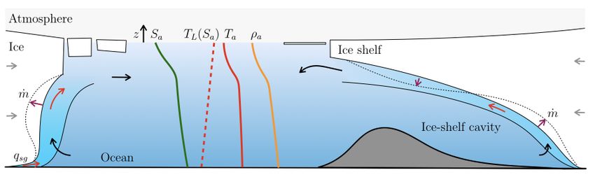
1. INTRODUCTION
                          A large fraction of the meltwater from the Earth’s ice sheets is discharged directly into the
                          ocean at depth. It initiates buoyant plumes that rise up the ice-ocean interface, mixing
                          with ambient ocean water. The dynamics of these plumes are important in regulating the
                          heat transfer that drives submarine melting, and in controlling the depth at which glacial
                          meltwater is exported to the open ocean. They are therefore a crucial factor in both the ice-
                          sheet response to ocean warming (Joughin et al. 2012), and the ocean response to ice-sheet
                          melting (Straneo & Heimbach 2013).
                              Plumes form both at the near-vertical front of tidewater glaciers and beneath relatively
                          shallow-sloping ice shelves (figure 1). The former are typical of the Greenland ice sheet,
                          Alaska and Svalbard, while the latter are typical of the margin of the Antarctic ice sheet. At
                          tidewater glaciers, plume-driven melting affects the shape of the front, so also plays a role
Submarine melting:        in ice-berg calving. Beneath ice shelves, both melting and freezing (due to the ‘ice pump’;
Melting from an ice       Lewis & Perkin 1986) affect the shape of the ice shelf, which has an important buttressing
front or ice shelf.
                          effect on the location of the grounding line and the ice flow across it.
Tidewater glacier: A          The ocean water adjacent to the ice sheets is typically within a few degrees of the
glacier that
terminates in the         freezing point, but is a mix of waters with different origins and properties. In Greenland,
ocean.                    outlet glaciers terminate in narrow fjords that are typically hundreds of meters deep. The
Grounding line: The       fjord water is often stratified, with relatively cold and fresh Polar Water overlying warmer
boundary between a        and saltier Atlantic Water (Straneo et al. 2012). The plumes themselves play a role in
grounded ice sheet        controlling the circulation in the fjords and the exchange of water with the continental
and floating ice          shelf (Straneo & Cenedese 2015). In Antarctica, a number of different water masses enter
shelf.                    beneath the ice shelves (Jacobs et al. 1992, Jenkins et al. 2016). These include Shelf Water,
Ice-shelf cavity: The     which is close to the surface freezing point and has high salinity due to sea-ice formation,
part of the ocean         Antarctic Surface Water, which is also cold but less dense, and Circumpolar Deep Water,
beneath a floating
ice shelf.                which is relatively warm and salty but is only able to intrude ice-shelf cavities in certain
                          locations, due to the topography of the continental shelf and wind forcing.
                              Subglacial plumes have similarities with turbulent plumes in other contexts, but some

                          Figure 1
                          Plumes occur at the front of tidewater glaciers and beneath floating ice shelves. Subglacial
                          discharge qsg and submarine melting ṁ produce buoyant water that rises up the ice front,
                          entraining warmer ocean water. Typical profiles of ambient salinity, temperature and density are
                          shown. The plume controls the melt rate and hence the shape of the ice-ocean interface. It can
                          reach a level of neutral buoyancy and separate from the ice front, controlling the depth at which
                          glacially modified water is exported to the open ocean. Decompression raises the freezing point so
                          the plume can become supercooled, resulting in freeze-on of marine ice to the ice-shelf base (the
                          ‘ice pump’) and creating cold waters that subsequently sink to produce Antarctic Bottom Water.

                      2   I. J. Hewitt
distinguishing features that make them fascinating in their own right. They are wall-
bounded flows in a stratified environment, initiated by a line or point source of subglacial
discharge, and sustained by a distributed source of buoyancy from submarine melting.
Importantly the boundary is reactive, so both its shape and the distributed buoyancy
source are coupled to the dynamics of the plume.
The question of the rise-height of a plume, and intrusion at a depth of neutral buoyancy,
is related to work on thermals and volcanic plumes (Woods 2010). The wall-bounded nature
of the flow, and to some extent the reactive boundary, have similarities with self-accelerating
turbidity currents (Parker et al. 1986, Meiburg & Kneller 2010). Some plumes are also large
enough to be affected by rotation, and they bear a number of similarities with katabatic
winds (Van den Broeke & Van Lipzig 2003). Related dynamics also occur in the context of
ventilation (Cooper & Hunt 2010).
This review focusses primarily on theoretical descriptions of subglacial plumes, which
have built on the classical theory of plumes and gravity currents (Morton et al. 1956, Turner
1979). We touch on laboratory experiments and field observations, and attempts to include
plume dynamics in larger-scale numerical models.
2. BACKGROUND
2.1. Equation of state
At conditions relevant to the polar oceans, the density of sea water increases with salinity
S and decreases weakly with temperature T (figure 2a). A linear approximation is usually
adopted. The normalised density deficit - or ‘buoyancy’ - with respect to ambient salinity
Sa and temperature Ta , is
∆ρ ρa − ρ
= = βS (Sa − S) − βT (Ta − T ), (1)
ρo ρo
where ρo is a reference density, βS is the haline expansion coefficient, and βT is the thermal
expansion coefficient. Note that g 0 = ∆ρ g/ρo is the reduced gravity often used to describe
buoyancy, but we use ∆ρ for greater consistency with the literature on subglacial plumes.
The relevant water masses are within a few degrees of the freezing point, whereas salinity
can vary considerably, so it is salinity that exerts primary control on the bouyancy.
The freezing temperature (the liquidus) depends on salinity and pressure, and is usually
expressed as a linear function,
TL (S, z) = To + λz − ΓS, (2)
where To is a reference, λ is the slope of the freeing-point with depth (z, positive upwards)
and Γ is the dependence on salinity. We suppress the argument z and write TL (S), but
note that the depth dependence is significant (the freezing point is depressed by 0.76 C at
1000 m depth). A useful concept is the temperature excess - or ‘thermal driving’ - defined
as the difference between the temperature and the local freezing point,
∆T = T − TL (S). (3)
(To avoid confusion, it is worth clarifying that the use of ‘∆’ here is different from in (1);
∆ρ denotes difference from ambient conditions, while ∆T denotes difference from the local
liquidus; ∆ is never used as a quantity on its own).
www.annualreviews.org • Subglacial Plumes 33 4
1022
1024
1026
1028
2
3
1
0 2
-1
1
-2
-3 0
26 28 30 32 34 36 0 1 2 3 4
Figure 2
(a) Density contours of sea water in conditions relevant to the polar oceans at atmospheric
pressure. Addition of fresh water causes mixing along the red line. Addition of ice at its freezing
point causes melting and consequent mixing along the purple line. Both lead to a decrease in
density. The thick black line is the liquidus, and the thinner line is the liquidus at 1000 m depth.
(b) Melt-rate coefficient M = ṁ/U as a function of temperature excess ∆T = T − TL (S) in the
three-equation formulation, for salinities in the range 0 to 35 g kg−1 (at 5 g kg−1 intervals). The
dashed line shows the two-equation formulation (11). Parameter values from Table 1.
Table 1 Typical parameter values.
1/2
βS 7.86 × 10⁻⁴ g 9.8 m s−2 StT = Cd ΓT 1.1 × 10⁻³
1/2
βT 3.87 × 10⁻⁵ C−1 c 3974 J kg C−1 StS = Cd ΓS 3.1 × 10⁻⁵
To 8.32 × 10⁻² C ci 2009 J kg C−1 1/2
St = Cd ΓT S 5.9 × 10⁻⁴
λ 7.61 × 10⁻⁴ C m−1 L 3.35 × 10⁵ J kg−1 E0 3.6 × 10⁻²
Γ 5.73 × 10⁻² C Cd 2.5 × 10⁻³ α 0.1
Values of Stanton numbers are those suggested by Jenkins et al. (2010b), which have been widely adopted.
Drag coefficient and entrainment rate are also quite uncertain; these represent commonly used values.
2.2. Buoyancy sources
Two distinct sources of buoyancy are important: subglacial discharge, and submarine melt.
Subglacial discharge is meltwater that is sourced from the surface or base of the grounded
ice sheet. It is essentially fresh, and emerges close to the pressure-dependent freezing point.
It is therefore considerably lighter than the ambient water, with density deficit
∆ρsg /ρo = βS (Sa − Si ) − βT (Ta − TL (Si )) ≈ 0.028, (4)
for Sa = 35 g kg−1 and Ta = 0 C (the value changes little over a range of ambient conditions
and can essentially be treated as constant). For notational convenience we have introduced
the salinity of the ice (and subglacial discharge), Si ≈ 0. Adding such water to cold ocean
water causes mixing along an almost horizontal line in T -S space (figure 2a).
Submarine melt occurs directly into the ocean. This similarly provides a source of fresh
water, but because the energy required for the phase change must come from the ocean
itself, it also causes substantial cooling. Accounting for the latent heat L plus the energy
required to first warm the ice from temperature Ti to its melting point, this meltwater can
4 I. J. HewittSUBGLACIAL DISCHARGE
This is meltwater produced at the base of a glacier by geothermal or frictional heating, or meltwater from the
glacier surface that is routed to the base through crevasses and moulins. It is possible that some discharge
emerges at intermediate depths through englacial channels, but most is thought to travel along the interface
between ice and substrate, emerging at the base of the ice front or grounding line.
Distribution. Subglacial water flow is driven by a hydraulic potential, controlled primarily by ice surface
elevation (Cuffey & Paterson 2010, Fountain & Walder 1998). It follows roughly the same flow lines as the
ice. Some of the flow may be distributed widely across the bed, in permeable sediments or linked cavities
that form as ice slides over its substrate. However, much of the flow is concentrated in tunnels - Röthlisberger
channels - incised upwards into the ice. These tunnels are enlarged through dissipation-driven melting of
their walls, counteracted by viscous creep when the subglacial water pressure is less than the pressure in
the ice. The partitioning of subglacial discharge between distributed and point sources is largely unknown.
Observations of isolated plumes (eg Mankoff et al. 2016) and localised undercutting (eg Fried et al. 2015)
indicate that a substantial part of it is channelised - at least in places with large discharge - but the extent
of distributed discharge across the rest of the ice front is still uncertain.
Magnitude. Direct measurement of subglacial discharge is challenging, so it is usually estimated based on
upstream sources. The order of magnitude of basal melting beneath grounded ice sheets is 1 − 10 mm y−1 .
Over a flow-line distance of, say, 300 km this gives typical discharge on the order of 10−5 − 10−4 m2 s−1 per
unit width, not accounting for convergence from a wider catchment. Surface melting occurs at typical rates
of 1 − 10 m y−1 over distances on the order of 30 km, giving larger fluxes on the order of 10−3 − 10−2 m2 s−1
averaged over the year. Integrating over catchment basins, estimates of summer discharge beneath Greenland
glaciers are on the order of 10 − 1000 m3 s−1 , entering fjords of width 1 − 10 km (eg Carroll et al. 2016).
Timing. In Greenland there is a strong seasonal cycle of surface melting that dominates subglacial dis-
charge. There can be a time lag of days to weeks between melting and discharge, due to temporary storage in
supraglacial lakes and the subglacial drainage system, especially early in summer when the drainage system
is less developed (eg Chandler et al. 2013). In Antarctica, where discharge is sourced from basal melting,
there is no reason to expect a seasonal signal. Filling and drainage of subglacial lakes (with a timescale of
months to years) have shown that drainage is nevertheless unsteady, and episodic discharge events are likely
(eg Fricker et al. 2007, Stearns et al. 2008). There are also likely to be tidal modulations, since tides control
the hydraulic potential close to the grounding line.
be considered to have an effective temperature excess
Modified latent heat:
L + ci (TL (Si ) − Ti ) L̃ The energy L̃ =
∆Tief =− =− , (5) L + ci (TL (Si ) − Ti )
c c
accounts for the
and an effective meltwater temperature Tief = TL (Si )+∆Tief . Here ci and c are the specific latent heat as well as
heat capacity of ice and water respectively. The quantity ∆Tief is a proxy for the modified warming ice at
temperature Ti to
latent heat L̃, and takes values . −84 C. Submarine melting therefore causes mixing along its melting point.
a steeper line in figure 2a (Gade 1979). The effective density deficit,
∆ρef ef
i /ρo = βS (Sa − Si ) − βT (Ta − Ti ) ≈ 0.024, (6)
www.annualreviews.org • Subglacial Plumes 5is slightly reduced, but is still dominated by the effect of freshening. (This definition of ∆Tief
differs slightly from some literature, where it is related to the interfacial temperature; the
magnitude of the latent heat makes the difference negligible).
2.3. Melting
We refer to the phase change at the ice–water interface as melting, though it may be more
proper to call it dissolving or ablating, since salt transport at the interface is important
(Woods 1992, Kerr & McConnochie 2015). Most of the development of parameterisations
for melting at a glacier–ocean interface has been by analogy with melting beneath sea ice,
for which more observations are available (McPhee 2008). However, the extrapolation from
an essentially horizontal interface in that setting to the sloping interface of ice shelves or
glacier fronts is the subject of some uncertainty and current debate. Useful discussions are
given by Holland & Jenkins (1999) and Jenkins et al. (2010b).
2.3.1. Three-equation formulation. The ice–water interface is assumed to be in local ther-
modynamic equilibrium, so its temperature Tb and salinity Sb satisfy
Tb = TL (Sb ). (7)
Heat and salt balances at the interface require that
ṁ (L + ci (Tb − Ti )) = FT , ṁ(Sb − Si ) = FS , (8)
where ṁ is the melt rate (m s−1 ), and FT and FS are the fluxes of heat and salt from
the water to the interface. The terms proportional to ci represent an approximation of the
conductive heat flux from the interface into the ice. The heat balance can also be written
in terms of the effective temperature defined in (5); making use of the good approximation
Tb − TL (Si )
L̃/c, it becomes ṁc(Tb − Tief ) = FT . If the heat and salt fluxes were known,
(7)-(8) together determine the melt rate ṁ and the interfacial properties Tb and Sb .
The fluxes are usually related to temperature T and salinity S evaluated outside of
interfacial boundary layers,
FT = γT c(T − Tb ), FS = γS (S − Sb ), (9)
where c is the heat capacity of the water, and γT and γS are transfer coefficients, having units
of velocity. The most suitable form of these coefficients is not yet established. It is commonly
1/2
p
assumed that they are proportional to the friction velocity U∗ = τ /ρo = Cd U , defined
in terms of interfacial shear stress τ and related by a drag coefficient Cd to the velocity U
(outside a viscous boundary layer). In that case we write γT = ΓT U∗ and γS = ΓS U∗ , or
1/2 1/2
γT = StT U and γS = StS U , where StT = Cd ΓT and StS = Cd ΓS are thermal and saline
Stanton numbers, which are assumed constant in most recent work (Jenkins et al. 2010b).
This constitutes the so-called three-equation formulation used in many models. It gives rise
to a melt rate of the form ṁ = M U , where M (T, S) is a melt-rate coefficient depending on
temperature and salinity (figure 2b).
In the context of a subglacial plume, the velocity U is usually taken to be the plume
velocity, but in some situations this has been supplemented or replaced by a background
value to represent tidal currents, whose amplitude may be larger than the mean flow of
the plume. Jenkins et al. (2010b) suggest taking U∗2 = Cd (U 2 + Utidal 2
), where Utidal is the
root-mean-square of the tidal currents.
6 I. J. Hewitt2.3.2. Two-equation formulation. An alternative description (McPhee et al. 2008) uses an
approximate heat balance,
ṁ (L + ci (TL (S) − Ti )) = St U c(T − TL (S)), (10)
in which the interfacial temperature Tb = TL (Sb ) is replaced by the freezing point of the
water outside of the interfacial boundary layer TL (S), and a lumped Stanton number St =
1/2
Cd ΓT S is adopted. This has been fitted to data from beneath the Ronne ice shelf and,
at least with the limited constraints available, seems to work just as well as the seemingly
more fundamental three-equation model (Jenkins et al. 2010b).
Making the good approximation TL (S) − TL (Si )
L̃/c, this melt rate can be expressed
simply as a product of velocity and thermal driving ∆T = T − TL (S),
c∆T
ṁ = St U . (11)
L̃
When expressed in terms of ∆T (rather than T ) and S, the three-equation formulation also
gives an approximately linear dependence on ∆T , with much weaker dependence on the
salinity (figure 2b). The expression (11) is therefore a useful simplification, and is adopted
in the plume models in section 3.
2.3.3. Alternative formulations. The above parameterisations make the assumption that
the velocity scale in the transfer coefficients is inherited, via the friction velocity, from
the fluid velocity near the interface. An interpretation is that the width of the laminar
sublayer, across which salt and heat must ultimately diffuse, is set by the shear stress
exerted by fluid motion outside of the sublayer (Holland & Jenkins 1999, Wells & Worster
2008, McConnochie & Kerr 2017a). When the interface is sloped rather than horizontal,
there is an alternative possibility that this width is set by the sublayer itself becoming
buoyantly unstable. The lightest fluid is at the interface, so if that interface is sloped
(and most obviously if it is vertical), the sublayer will be unstable to convection once its
thickness δ exceeds a certain size. This can be interpreted as reaching a critical value Rac
of the local Rayleigh number Ra = ∆ρb gδ 3 /νDS , where ∆ρb /ρo = βS (S − Sb ) − βT (T − Tb )
is the density difference across the sublayer. In that case, the transfer coefficients would
1/3
be independent of the external fluid velocity, and would scale with 1/δ ∝ ∆ρb . It can be
shown (Kerr & McConnochie 2015) that one expects ∆ρb ∝ ∆T , at least for small thermal
driving, and the resulting melt rate therefore scales as ṁ ∝ ∆T 4/3 , independent of velocity.
Wells & Worster (2008) developed a detailed model for a plume rising up a vertical
wall, which suggests two transitions: first from a laminar state to a turbulent regime with
sublayer width set by the buoyancy argument just given, and then to a second turbulent
regime with sublayer width set by the shear stress of the turbulent outer flow, determined by
a critical Reynolds number. The second transition occurs where the velocity is sufficiently
large that the shear-driven criteria gives a narrower sublayer (it can also be thought of in
terms of a critical value of the Rayleigh number on the length scale of the plume). That
study was for the simpler situation of a single component controlling buoyancy, but Kerr &
McConnochie (2015) have suggested how the argument can be extended to the present case.
McConnochie & Kerr (2017a) found that for a vertical interface the transition to a shear-
driven sublayer happens above a velocity of about 4 cm s−1 , and the velocity-dependent
parameterisations described above may be appropriate in that case, at least in form.
www.annualreviews.org • Subglacial Plumes 7LABORATORY EXPERIMENTS
There have been a number of experiments on the melting of vertical ice faces (Huppert & Turner 1980,
Josberger & Martin 1981, Kerr & McConnochie 2015, Cenedese & Gatto 2016a). Due to size limitations, the
experiments do not necessarily access the same turbulent regime that is thought to be relevant to large-scale
geophysical flows. However, Kerr & McConnochie (2015) found good agreement with a uniform velocity-
independent melt rate, ṁ ∝ ∆T 4/3 . Experiments with an additional line source of buoyancy, and therefore
higher velocities, showed a hint that the melt rate starts to scale with velocity (McConnochie & Kerr 2017b),
possibly accessing the shear-driven boundary layer regime discussed in section 2.3.3. In stratified water,
Huppert & Turner (1980) and McConnochie & Kerr (2016a) found layered outflows, interpreted as double-
diffusive behaviour associated with different widths of thermal and solutal boundary layers. Experiments
in a two-layer ‘ocean’ with a point source of ‘subglacial discharge’ (Cenedese & Gatto 2016a) showed that
overall melting increases with the strength of the source, and that the plume may intrude both at the surface
and at the density interface, in qualitative agreement with theoretical expectations and field observations.
Direct Numerical Simulations. Gayen et al. (2016) solved the Navier-Stokes equations for the turbulent
flow at a vertical ice-water interface on a similar scale to that achieved in the laboratory. They found good
agreement with the experiments of Kerr & McConnochie (2015), consistent with buoyancy controlling the
width of the interfacial sublayer. Mondal et al. (2019) extended the computations to sloping interfaces.
2.4. Freezing
Freezing directly onto the ice-ocean interface can be described by the same heat and salt
balances as in (8). However, the melting and freezing process is not symmetric (salt rejection
produces denser water at the interface rather than lighter) and appropriate values of the
transfer coefficients may therefore differ, perhaps significantly (McPhee et al. 2008). In the
context of a subglacial plume, freezing is driven by upwelling water becoming supercooled
due to the depth-dependent freezing point. Such supercooling has potential to produce
frazil ice in suspension, so marine ice can grow by the precipitation of buoyant ice crystals,
as well as freeze-on directly to the interface. This is discussed in section 5.4.
3. ONE-DIMENSIONAL PLUMES
Some very useful insights and scaling arguments can be derived from simple one-dimensional
models. These were originally developed for plumes beneath ice shelves by MacAyeal (1985)
and Jenkins (1991), adapting earlier models of turbudity currents (eg Turner 1986). The
framework described here follows most closely the work of Jenkins (2011) and Magorrian
& Wells (2016).
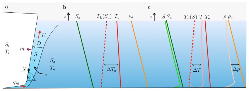
The situation considered is shown in figure 3. The coordinate X lies along the ice–ocean
interface, with sin φ = dz/dX being the local slope. Ultimately one would like to know the
evolution of the ice–ocean interface, but the timescales over which this occurs are longer
than those on which the plume evolves, allowing us to consider the steady-state behaviour
of the plume - and the resulting melt rates - for a given ice geometry. We mostly have in
mind a vertical ice front (φ = π/2), but the model is applicable to shallower slopes too.
The plume is described in terms of its thickness D, average speed U , salinity S and
8 I. J. HewittFigure 3
(a) A one-dimensional plume with velocity U , thickness D, salinity S and temperature T . (b)
Typical profiles of ambient salinity, liquidus, temperature and density together with ambient
temperature excess ∆Ta . (c) Lighter colours show typical properties of the plume.
temperature T , for which top-hat profiles are assumed (alternative shape-factors are possi-
ble and would lead to similar equations with modified coefficients). Making a Boussinesq
assumption, conservation equations for mass, momentum, salt and heat are
∂ ∂
DU 2 = D∆ρ g sin φ/ρo − Cd U 2 ,
(DU ) = ė + ṁ, (12)
∂X ∂X
∂ ∂
(DU S) = ėSa + ṁSi , (DU T ) = ėTa + ṁTief . (13)
∂X ∂X
Here ė is the entrainment rate of ambient water and ṁ is the melt rate. The conventional
entrainment assumption is that ė = EU , where E is an entrainment coefficient. This
depends on a competition between shear-induced turbulence and the stabilising effect of
mixing across a density interface (Ellison & Turner 1959, Turner 1986). A simple model
is E = E0 sin φ, where the inclusion of the slope attempts to account for this competition
(Bo Pedersen 1980), but alternative parameterisations dependent on Richardson number
have also been used (eg Holland et al. 2007). The melt rate ṁ is given in terms of U , T
and S by one of the parameterisations described in section 2.3.
The driving force due to buoyancy in (12)2 can also have a component due to gradients
in plume thickness, which allows the flow to become subcritical on shallow slopes. That
term is neglected here on the basis of the plume thickness being small. Turbulent wall drag
is parameterised with the drag coefficient Cd , usually taken to have a value around 0.0025
(although there appears little observational constraint on this). The salinity and tempera-
ture equations have effectively been integrated across the ice–ocean boundary, making use
of the flux boundary conditions (8).
The melt rate is found to be insignificant compared with the rate of entrainment and
can reasonably be neglected in (12)1 , though it plays an important role in (13) because
the meltwater’s salinity and temperature deficit are large. Making that simplification, it is
useful to re-write the model in terms of density deficit ∆ρ and temperature excess ∆T ,
∂
(DU ) = EU, (14)
∂X
∂
DU 2 = D∆ρ g sin φ/ρo − Cd U 2 ,
(15)
∂X
www.annualreviews.org • Subglacial Plumes 9∂ dρa
Density deficit: (DU ∆ρ) = ṁ∆ρef
i + sin φ DU, (16)
∆ρ = ρa − ρ ∂X dz
Difference from ∂
(DU ∆T ) = EU ∆Ta + ṁ∆Tief − λ sin φ DU. (17)
ambient density. ∂X
Sometimes referred We summarise some simple solutions to this model below. The effective meltwater buoyancy
to as buoyancy.
∆ρef
i and temperature excess ∆Ti
ef
are essentially constants, given by (5) and (6). The
Temperature excess: ambient thermal driving ∆Ta = Ta − TL (Sa ) will generally vary with depth; it is assumed
∆T = T − TL (S)
known here, with initial value ∆Ta0 . The final terms in (16) and (17) account for ambient
Temperature above
local freezing point. stratification and the depth-dependence of the freezing point.
Also called thermal
driving.
3.1. Plumes driven by subglacial discharge
If the plume is fed by subglacial discharge (per unit width) qsg , the most important driver is
the initial buoyancy flux qsg ∆ρsg . In some cases this may be sufficiently large that melting
of the ice face (the first term on the right of (16)) has a negligible effect on buoyancy, and
the plume dynamics are then decoupled from melting. The subglacial mass flux itself is
usually insignificant compared to the entrained water mass, so the situation is essentially
an ‘ideal’ plume (Turner 1979), in which U and ∆T adjust rapidly from their inlet values.
3.1.1. Uniform ambient. If the ambient conditions are uniform, the slope of the ice front is
constant, and we neglect depth-dependence of the freezing point, the solution has linearly
increasing thickness, constant velocity and temperature excess, and decreasing buoyancy,
1/3
qsg ∆ρsg g sin φ qsg E
D = E X, U = , ∆ρ = ∆ρsg , ∆T = ∆Ta0 , (18)
ρo (E + Cd ) DU E + St
where in the final term we have made use of the melt-rate approximation (11) for which
ṁ = U St c∆T /L̃. This implies a constant melt rate that varies linearly with the ambient
thermal driving and with the one-third power of the subglacial discharge (Jenkins 2011),
1/3
ESt c∆Ta0 qsg ∆ρsg g sin φ
ṁ ∼ . (19)
E + St L̃ ρo (E + Cd )
This makes clear the combined influence of entrainment E (which controls how fast heat is
transferred from ambient water to the plume) and Stanton number St (which controls how
fast heat is transferred from plume to interface). Note that Cd
E is likely for vertical ice
faces, and wall drag could reasonably be neglected in that case. For shallower slopes, when
entrainment is reduced, wall drag can be the dominant factor limiting plume velocity.
3.1.2. Linear stratification. The length scale over which the buoyancy flux is lost due to
ambient stratification is (from balancing first and last terms in (16))
1/2 1/3 −1/2
1 E + Cd qsg ∆ρsg g sin φ g dρa
`ρ = . (20)
sin φ E ρo (E + Cd ) ρo dz
Inserting this length scale into the uniform ambient solution (18) defines scales for each of
the variables, and the model can then be cast in dimensionless form by writing, for example,
X = `ρ X̂, D = E`ρ D̂(X̂), etc. The resulting scaled variables (with hats) satisfy
∂ ∂
D̂Û = Û , D̂Û 2 = (1 + Ĉd )D̂∆ρ̂ − Cˆd Û 2 , (21)
∂ X̂ ∂ X̂
10 I. J. Hewitt3
2
2.5
1.5 2
1.5
1
1
0.5
0.5
0 0
0 2 4 0 0.5 1 -1 0 1 2 0 2 4 0 0.5 1 -1 0 1 2
Figure 4
(a) Scaled solutions to (21)-(22) for a subglacially-driven plume with linear ambient stratification.
Variable scales are given by inserting the length scale (20) into (18). (b) Scaled solutions for a
plume with no subglacial discharge and linear ambient stratification. Variable scales are given by
inserting the length scale (27) into (24). In both cases ∆Ta = ∆Ta0 and Cd /E = 0.069 (darkest
colours, appropriate for a vertical ice face), 0.69 and 6.9 (lighter colours, for shallower slopes with
reduced entrainment). Both solutions also have ∆T̂ = 1 and ṁ ˆ = Û ∆T̂ . Dashed lines show the
unstratified solutions (18) and (24).
∂ ∂
ˆ )Û ∆T̂a − St
ˆ ṁ,
ˆ
D̂Û ∆ρ̂ = −D̂Û , D̂Û ∆T̂ = (1 + St (22)
∂ X̂ ∂ X̂
where Ĉd = Cd /E, St ˆ = St /E, ∆T̂a = ∆Ta /∆Ta0 , and ṁ ˆ = Û ∆T̂ for the melt-rate
parameterisation (11). Solutions to this scaled model are shown in figure 4a.
Of interest are the position Xneg ≈ 1.44`ρ at which the plume becomes negatively
buoyant, and the position Xstop ≈ 2.06`ρ at which it comes to rest (inertia enables it
to continue beyond the height of negative buoyancy). The plume water is at that point
denser than its surroundings and can be expected to intrude and sink to a neutral height
somewhere between the heights corresponding to Xstop and Xneg (Magorrian & Wells 2016).
The properties of this glacially-modified water are a mix of the subglacial discharge and
ambient water that has been entrained.
3.1.3. Two-layer stratification. In some cases, particularly in Greenland fjords, a two-layer
uniform stratification may be a better approximation of the ambient conditions. In that
case the solution (18) can be used for the lower layer, with the buoyancy ∆ρ undergoing
a sudden decrease at the density interface, by an amount equal to the ambient density
change. If ∆ρ is subsequently negative, the plume will decelerate and after an overshoot
can be expected to intrude along the density interface (Straneo & Cenedese 2015).
www.annualreviews.org • Subglacial Plumes 113.2. Plumes driven by submarine melting
The buoyancy flux provided by submarine melting becomes more important than that
provided by subglacial discharge after a length scale
1/3 2/3 2/3
qsg ∆ρsg ρo (E + Cd ) E + St L̃∆ρsg qsg
`sg = ef
= . (23)
ṁ∆ρi g sin φ ESt c∆Ta0 ∆ρef
i
This can vary substantially depending on the magnitude of subglacial discharge and the
ambient temperature, but obviously goes to zero for the limit qsg = 0 which we now consider.
For greater length scales, buoyancy comes from melting of the ice face and the dynamics are
inherently tied to the thermodynamics. One can also expect these submarine-melt-driven
plumes to occur above the intrusion height of the subglacially-driven plumes described in
the previous section (in the less dense upper layer of Greenland fjords, for example).
3.2.1. Uniform ambient. For uniform conditions, neglecting depth-dependence of the freez-
ing point, and assuming the melt rate parameterisation (11), the solution has increasing
thickness and velocity, with constant buoyancy and temperature excess determined by a
balance between entrainment and melting (Magorrian & Wells 2016),
1/2
2 E∆ρg sin φ St c∆T E
D = E X, U = 3 X 1/2 , ∆ρ = ∆ρefi , ∆T = ∆Ta0 .
3 ρo (2E + 2 Cd ) E L̃ E + St
(24)
The corresponding melt rate increases with the square root of distance,
3/2 !1/2
∆ρef
ESt c∆Ta0 i g sin φ
ṁ ∼ X 1/2 . (25)
E + St L̃ ρo (2E + 32 Cd )
The dependence on ambient thermal driving is stronger than for the subglacially-dominated
plume, because of the feedback of melting on plume buoyancy and hence speed.
This solution is exact if there is no subglacial discharge. If there is subglacial discharge
there is a smooth transition from the behaviour in (19) for X
`sg to that in (25) for
X
`sg . The melt rate always increases with distance during this transition, and is always
greater at any given position for larger subglacial discharge.
Note that because of the coupling between melting and buoyancy, this solution is only
appropriate if melt rate is proportional to plume velocity. If plume velocities are small, a
different (eg. tidal) velocity may control melting, as discussed in section 2.3. If the melt
rate is instead assumed constant, the appropriate solution is (McConnochie & Kerr 2016b)
!1/3 !1/3
5
3 ṁ∆ρef i g sin φ 1/3 4 ρo ( 4 E + Cd ) ṁ2/3 ∆ρef
i
D = E X, U = 5 X , ∆ρ = ef
.
4 ρo ( 4 E + C d ) 3 ∆ρi g sin φ EX 1/3
(26)
3.2.2. Linear stratification. Returning to the solution in (24), the ambient stratification
becomes important on a length scale
−1
St c∆Ta0 ∆ρef
i dρa
`ρ = , (27)
E + St L̃ sin φ dz
over which the buoyancy is reduced. Inserting this length scale into (24) determines suitable
values with which to scale each of the variables in this case. Following the same procedure
12 I. J. Hewitt6
5
4
3
2
1
0
0 5 0 1 2 -1 0 1 2 -2 0 2 -1 0 1
Figure 5
Scaled solutions for a plume with depth-dependence of the freezing point, no subglacial discharge
and uniform ambient conditions. Here ∆Ta = ∆Ta0 , Cd /E = 0.069 (darkest, vertical slope), 0.69
and 6.9 (lighter, shallower slopes) and St /E = 0.016, 0.16 and 1.6. Variable scales are given by
inserting the length scale (28) into (24). Dashed lines show the solution not accounting for the
freezing point change (24).
as earlier, this leads to a similar set of dimensionless equations that depends only on the
ratio Ĉd = Cd /E and ∆T̂a = ∆Ta /∆Ta0 . Solutions for uniform ambient temperature are
shown in figure 4b. The buoyancy falls off almost linearly, resulting in a decrease in velocity
and hence melting. The plume becomes negatively buoyancy at a distance Xneg ≈ 2.25`ρ ,
and stops at a distance Xstop ≈ 2.85`ρ (these numerical values are specific to the value of
Ĉd , as seen in the figure). Magorrian & Wells (2016) suggest that another similar plume is
initiated at Xstop , and one can expect a sequence of such plumes to develop, each intruding
at successively greater heights and forming a ‘layered’ structure that would presumably
interfere with the ambient water column in a non-trivial way.
3.2.3. Depth-dependence of the freezing point. The depth-dependence of the freezing point
becomes important on the length scale
∆Ta0
`T = . (28)
λ sin φ
Inserting this length in (24) to define variable scales produces another dimensionless model
that depends only on Ĉd = Cd /E, St ˆ = St /E, and ∆T̂a = ∆Ta /∆Ta0 (reverting to the
unstratified case). Solutions are shown in figure 5 for uniform ambient thermal driving.
The temperature excess of the plume becomes negative after a distance Xf reeze , causing
supercooling and consequent freeze-on (negative ṁ). Freeze-on reduces the buoyancy, so the
plume becomes negatively buoyant and then stops. Note that this model treats freeze-on
simply as negative melting and ignores the role of frazil ice discussed in section 5.4.
3.3. Point sources of subglacial discharge
If subglacial discharge emerges from a channelised drainage system it acts more like a point
source than a line source. This gives rise to a plume that is more conical in shape, and a
www.annualreviews.org • Subglacial Plumes 13simple model is to treat such plumes as half of a classical axisymmetric plume (Kimura et al.
2014, Cowton et al. 2015, Slater et al. 2016). Direct numerical simulations of such a plume
lend some support to this approach (Ezhova et al. 2018). With appropriate modifications
to account for the area undergoing entrainment and the area in contact with the ice, and
writing b for the radius of the half cone, the model is
∂ π 2
∂ π 2 2
π 2
2
b U = απbU, 2
b U = 2
b ∆ρg/ρo , (29)
∂X ∂X
∂ π 2 dρa π 2 ∂
= 2bṁ∆ρef π 2
2
b U ∆ρ i + b U, b U ∆T = απbU ∆Ta . (30)
∂X dz 2 ∂X 2
The entrainment coefficient in this case is conventionally written as α. We have specialised
to the case of a vertical ice front (φ = π/2) and neglected both wall drag and the cooling
effect of melting, which are unlikely to be significant in that case, as well as the depth-
dependence of the freezing point.
As for a line plume the contribution of melting to buoyancy is initially insignificant, and
the buoyancy flux is conserved from the source. Over this region the ideal plume has
1/3
(Qsg ∆ρsg g)1/3
6α 5 9α Qsg ∆ρsg
b= X, U= 1/3
, ∆ρ = π 2 , ∆T = ∆Ta0 . (31)
5 6α 5π ρo X 1/3 2
b U
If the melt-rate parameterisation (11) is adopted, the total (volumetric) melt rate over a
depth H is
Z H 1/3 1/3
6 9α St c∆Ta0 Qsg ∆ρsg g
2bṁ dX ∼ H 5/3 . (32)
0 5 5π L̃ ρo
The melt rate again scales linearly with thermal driving, and with the one-third power of
the subglacial discharge.
For a localised source, it is more likely that the mass flux itself is significant too, and
there may be an appreciable depth `0 over which the plume is dominated by the subglacial
discharge. This can be accounted for using a virtual origin (Morton et al. 1956). The
plume’s velocity and thermal driving adjust over this scale, the latter increasing by dilution
from its initial value ∆Tsg ≈ 0, towards the ambient value ∆Ta0 . If `0 is a significant
fraction of H this cold region of the plume can weaken the dependence of melting on Qsg
(Slater et al. 2016). One can show that a linear stratification becomes important over a
1/4
length scale `ρ ∝ Qsg |dρa /dz|−3/8 , and the behaviour of plumes reaching their level of
neutral buoyancy can be analysed as in section 3.1 (Slater et al. 2016).
3.4. Melting rates
The results of these models can be used to infer the sensitivity of melting to different
parameters. Consider an example of a vertical ice front of width W = 2 km and depth
H = 500 m, with uniform ambient water at thermal driving ∆Ta0 = 4 C. If there is no
subglacial discharge the total (volumetric) melt rate from (25) is expected to scale as
3/2 !1/2
H
21/2 ∆ρef
Z
St c∆Ta0 i g
W ṁ dX ∼ H 3/2 W ≈ 4 m3 s−1 (ṁ ≈ 0.3 m d−1 ).
0 3E 1/2 L̃ ρo
(33)
14 I. J. HewittA point-source plume fed by subglacial discharge Qsg = 100 m3 s−1 would produce total
melt rate (32), around 1.2 m3 s−1 (ṁ ≈ 0.1 m d−1 ), and if the same subglacial discharge
were distributed over the width W , the melt rate from (19) would be
Z H 1/3
1 St c∆Ta0 Qsg ∆ρsg g
W ṁ dX ∼ HW 2/3 ≈ 20 m3 s−1 (ṁ ≈ 1.7 m d−1 ).
0 E 1/3 L̃ ρo
(34)
Total melting driven by the point source is relatively small compared with the background
melting of the rest of the ice front, and is dwarfed by the melting that would occur if the
same subglacial discharge were distributed across the bed. Useful scalings with widths,
depths, subglacial discharge, and thermal driving are derived from such expressions.
4. TWO-DIMENSIONAL PLUMES
A number of studies have considered two-dimensional extensions of the model in (12)-(13)
to investigate flow in ice-shelf cavities (eg Holland et al. 2007, Payne et al. 2007). Given
the application to shallow slopes, these are posed in horizontal Cartesian coordinates (x, y).
They consist of depth-integrated conservation equations (across the thickness of the plume),
analogous to shallow-water type models in other settings (eg Jungclaus & Backhaus 1994),
∂D
+ ∇ · (DU) = ė + ṁ, (35)
∂t
∆ρgD2
∂ ∆ρgD ∂d ∂
(DU ) + ∇ · (DUU ) − f DV = − − Cd |U|U + ∇ · (νD∇U ) , (36)
∂t ρo ∂x ∂x 2ρo
∆ρgD2
∂ ∆ρgD ∂d ∂
(DV ) + ∇ · (DUV ) + f DU = − − Cd |U|V + ∇ · (νD∇V ) , (37)
∂t ρo ∂y ∂y 2ρo
∂
(DS) + ∇ · (DUS) = ėSa + ṁSi + ∇ · (νD∇S) , (38)
∂t
∂
(DT ) + ∇ · (DUT ) = ėTa + ṁTief + ∇ · (νD∇T ) . (39)
∂t
Here ∇ = (∂/∂x, ∂/∂y) is the horizontal divergence, U = (U, V ) is the velocity, ν is an
eddy diffusivity, d(x, y) is the elevation of the ice-shelf base, and f = 2Ω sin ϕ is the Coriolis
parameter. Parameterisations of entrainment ė = E|U| and melt rate ṁ are also required.
4.1. The effects of rotation
The key feature of (35)-(39) that was ignored in the one-dimensional models is the Coriolis
force. On larger scales this is significant, and the dominant force balance in (36)-(37) is
geostrophic, between the final terms on the left hand side and the first terms on the right.
The plume flows predominantly across the slope (to the left in the Southern hemisphere)
rather than up it. Similar effects occur for katabatic winds (Van den Broeke & Van Lipzig
2003, Stiperski et al. 2007).
To illustrate the effect, figure 6 shows a plume beneath a linearly sloping ice shelf with
uniform ambient conditions and no subglacial discharge. Without rotation, this situation is
described by the one-dimensional solution (24), in which the plume had constant buoyancy
∆ρ and temperature excess ∆T . The plume thickness D grows linearly with x, and the
dominant force balance between buoyancy and wall drag causes the velocity to increase as
www.annualreviews.org • Subglacial Plumes 153 3
2 2
1 1
0 4
0 1
0 0
0 1 2 3 0 1 2 3
Figure 6
Solution for plume thickness, melt rate, and streamlines, for a linearly sloping ice shelf with
uniform ambient conditions, showing the effect of the Coriolis force (f < 0). These are steady
solutions to (35)-(39) ignoring the gradient of plume thickness and diffusion, with melt-rate (11),
and zero flux along x = 0 and y = 0. The solution is scaled using values in (24)-(25) with X = `f
from (40), and depends upon the single parameter Cd /E = 6.9. For x̂
1 the solution is as for a
one-dimensional plume (24). For x̂, ŷ
1 it asymptotes towards geostrophic balance (41).
U ∼ (∆ρ g sin φ/ρo Cd )1/2 D1/2 (E
Cd is assumed here). The Coriolis term takes over
from wall drag in balancing buoyancy once the plume is sufficiently thick, D ∼ Cd U/f ,
which means D ∼ Cd ∆ρ g sin φ/ρo f 2 (this scale is loosely equivalent to an Ekman layer
depth). Since D ∼ 32 Ex, this defines a length scale
2E + 32 Cd
∆ρ g sin φ
`f = , (40)
E ρo f 2
over which the effects of rotation become important (the additional factor of 2E accounts
for the possibility E ∼ Cd ). If the plume continues to thicken, drag becomes increasingly
insignificant, and the plume tends towards a geostrophic balance with U
V and
∆ρg sin φ
V =− . (41)
ρo f
In this case the plume is flowing across the slope and entrainment causes the thickness to
increase in that direction rather than up the slope (figure 6). Nevertheless there is still
a weak frictionally-driven upslope component to the flow, analogous to that in a bottom
Ekman layer. Clearly this leads to the collection of plume water at lateral boundaries, where
topography then plays a key role in diverting the flow (eg Payne et al. 2007). The linear
dependence of V on ∆ρ, which is itself proportional to ∆Ta (24), suggests that melting
should scale quadratically with thermal driving in this case (Holland et al. 2008).
The depth-integrated nature of these models means that they capture the competition
between friction and geostrophy in a rather crude sense. In reality there must be significant
vertical structure to the velocity (Wang et al. 2003, Cenedese et al. 2004), which could inter-
act with the melt-induced stratification in a non-trivial way (Jenkins 2016). Understanding
the structure of these large-scale plumes is an important area for future research.
16 I. J. Hewitt4.2. Interaction with ice shelf topography
Many ice shelves have channel-like features in their base (Rignot & Steffen 2008, Vaughan
et al. 2012, Mankoff et al. 2012). These channels act as a topographical focus for sub-shelf
plumes, with the possibility for enhanced melting and channel growth (Dutrieux et al. 2013,
Alley et al. 2016), but also potentially reducing average melt rates by shielding other areas
of the ice shelf (Millgate et al. 2013). The features may also act as zones of mechanical
weakness that facilitate fracturing (Dow et al. 2018).
One mechanism for forming such channels is through a feedback between the evolution
of ice-shelf topography and plume-driven melting. This possibility has been studied with
the two-dimensional model in (35)-(39) (Gladish et al. 2012, Sergienko 2013, Dallaston et al.
2015). Although there appears to be no inherent instability of an initially uniform ice shelf,
undulations in ice thickness inherited at the grounding line are found to grow downstream
due to focussed plume flow and melting. Lateral shear or non-uniform subglacial discharge
can have the same effect. This is consistent with some observed channels that line up
with expected locations of subglacial discharge (LeBrocq et al. 2013). Ice-shelf channels are
generally steeper on their western sides (Alley et al. 2016), consistent with the influence of
the Coriolis force that causes enhanced flow and melting on their western flanks.
Detailed measurements have revealed that in some of these channels the ice-shelf base
is not smooth but comprises hundreds-of-meter-wide ‘terraces’, separated by ∼ 45◦ steps
(Dutrieux et al. 2014). Melting is enhanced on the steep walls and varies from one terrace
to another. It is currently unclear what mechanism lies behind these distinctive features.
5. FURTHER ISSUES
5.1. Interaction with ambient flow
In the simple models discussed above the ambient ocean was assumed to be relatively
motionless, with properties that are somehow known. In reality there are tidal and other
currents, and the ambient properties are determined by the larger-scale ocean circulation,
which is driven in part by the plume. In the simplest picture, upwelling plumes drive an
overturning circulation, drawing in water from the open ocean at depth to replenish the
outflowing glacially-modified water. Such circulations appear to dominate some Greenland
fjords (eg Gladish et al. 2015), but not ubiquitously. The presence of a sill can limit exchange
with the continental shelf, and there are also tidal and wind-driven circulations (eg Jackson
et al. 2014, Straneo & Cenedese 2015). In Antarctica, horizontal circulation plays a bigger
role, and sea ice and wind forcing are significant in determining which water masses are
drawn into the ice-shelf cavities. A useful summary is provided by Jenkins et al. (2016).
5.2. Interaction with ice-front morphology and calving
Plume models typically assume a vertical ice front, but real ice fronts have a more compli-
cated geometry, partly due to non-uniform submarine melting (Fried et al. 2015). Slater
et al. (2017a) coupled plume dynamics with an evolving ice front and found steady undercut
profiles that depend on the magnitude of subglacial discharge. Undercutting of the ice front
can facilitate fracturing and ice-berg calving (eg O’Leary & Christoffersen 2013, Benn et al.
2017). This means that overall rates of ‘frontal ablation’ (melting and calving combined)
may be sensitive to the spatial pattern of melting, or perhaps its maximum, rather than
necessarily the area-average. Understanding the interplay of plume-driven melting with
www.annualreviews.org • Subglacial Plumes 17ice-front evolution and calving is an important area for future research.
5.3. Detrainment
In the top-hat models of sections 3 and 4, one-way entrainment was assumed and detrain-
ment to the ambient effectively occurs at a ‘point’ (Xstop ) where the plume runs out of
momentum and its thickness tends to infinity. Recent experimental studies have suggested
that detrainment into a stratified ambient can be a more continuous process (Baines 2005,
Cooper & Hunt 2010, Bonnebaigt et al. 2018), and that classical theories may need to be
modified to account for this. Continuous detrainment is associated with a density variation
across the plume, since denser fluid at the outer edge reaches neutral buoyancy earlier than
the core. The situation appears to be exacerbated for a distributed buoyancy source, since
lighter fluid is continually added to one side of the plume (Gladstone & Woods 2014). Hogg
et al. (2017) developed a model with a linear buoyancy profile across the plume, which
allows for ‘peeling’ detrainment. These studies raise the possibility that current models
for submarine-melt-driven plumes (including those in section 3.2 and section 4) are not
appropriate and need to be revised. This is again an important area for further work.
5.4. Frazil ice
Frazil ice forms in plume water that is supercooled as a result of decompression. Suspended
ice crystals increase buoyancy and can accelerate the plume, enhancing crystal growth. but
larger crystals also precipitate more rapidly, thereby reducing the buoyancy. This leads to
a complex interplay between nucleation, crystal growth, and plume dynamics. The effects
were included in the plume model of Jenkins & Bombosch (1995). Smedsrud & Jenkins
(2004) added multiple crystal size classes, Holland & Feltham (2006) extended it to two
dimensions, and Rees Jones & Wells (2018) introduced a continuous size distribution. The
main modification to the basic model (12)-(13) is to introduce the volume fraction of ice
crystals C, which adds a term (1 − ρi /ρo )C to the buoyancy (1). A conservation equation is
included for the crystals, with freezing rate f˙ and precipitation (settling) rate ṗ, the latter
of which adds to the thickness of the ice shelf along with the negative melting rate ṁ at the
interface. The ice fraction C is broken down into a distribution over crystal size, and f˙ and
ṗ are functionals of that distribution, whose form can have a large effect on the behaviour
of the plume (Smedsrud & Jenkins 2004, Rees Jones & Wells 2018).
5.5. Sediments
Subglacial discharge can transport significant quantities of glacially-eroded sediment, which
is deposited near the grounding line or ice front (eg Powell 1990, Drews et al. 2017). Sus-
pended sediment is also a visible indicator of surfacing plumes (eg Schild et al. 2016).
Sediment concentrations vary considerably, but estimates of Cs ∼ 1 − 10 kg m−3 in larger
subglacial channels are typical (eg Salcedo-Castro et al. 2013). The higher loads can provide
a significant contribution to buoyancy, adding a term (1/ρs − 1/ρo )Cs to (1), but only in
extreme cases (Cs & 40 kg m−3 ) would the subglacial discharge be negatively buoyant. The
sediments are clay, silt and sand, and their settling is complicated by flocculation of clay
particles in sea water (eg Sutherland et al. 2015). Mugford & Dowdeswell (2011) developed
a model of a sediment-laden subglacial plume to study deposition patterns, assuming negli-
gible effect on buoyancy. The effect of particles on plume dynamics have also been studied
18 I. J. HewittOBSERVATIONS OF PLUMES
Surfacing plumes at tidewater glacier fronts have been observed with both timelapse cameras and satellite
imagery, and used as indicators of subglacial discharge strength (eg Bartholomaus et al. 2016, Slater et al.
2017b). A number of recent studies have sampled oceanographic properties of plume water close to the ice
fronts (Stevens et al. 2016, Mankoff et al. 2016). Such measurements have allowed estimates of the amount
of mixing with ambient water and of submarine melting. Comparison with plume theory suggests that some
localised plumes may be better treated as finite-extent line plumes rather than point sources (Jackson et al.
2017), consistent with observations of large subglacial channel portals (Fried et al. 2015, Rignot et al. 2015).
In Antarctica, observations beneath the ice shelves are relatively limited. Oceanographic measurements
have been made using autonomous underwater vehicles (Jenkins et al. 2010a), but they are not able to
sample the water immediately adjacent to the ice-shelf base. Point measurements of the sub-shelf properties
have been made by drilling down through the ice (eg Nicholls et al. 1997). Detailed measurements of ice-shelf
melting rates have been made using phase-sensitive radar (Corr et al. 2002), and broader-scale estimates of
melting have been derived from satellite altimetry (eg Pritchard et al. 2012).
in volcanic and other contexts (eg Sparks et al. 1991, Woods 2010).
6. NUMERICAL MODELLING
6.1. Plume-resolving models
A number of recent studies have used general circulation models (GCMs) to explicitly
simulate plumes at a vertical ice front (eg Xu et al. 2012, 2013, Sciascia et al. 2013).
Typical resolution is around 1 − 10 m near the ice front. Turbulence is described with an
eddy diffusivity, whose size controls the rate of entrainment and which is typically fitted to
give rise to expected entrainment rates from plume theory. These studies have corroborated
many results of the plume theories in section 3.
Kimura et al. (2014) used a finite-element model to investigate subglacially-driven
plumes. An important finding was that the Coandă effect tends to keep the plume attached
to the vertical ice face, even if initiated with significant horizontal momentum. They also
found that overall melting increases if discharge is split between two channels, unless they
are close enough together for the plumes to merge in which case melting is lower due the
reduced area of the affected ice face (a result also found in the laboratory experiments of
Cenedese & Gatto (2016b)). Slater et al. (2015) considered discharge from multiple point
sources, finding that total melting increases if discharge is spread between more smaller
channels, but that the associated plumes are less likely to reach the surface in a stratified
environment. Again, this is consistent with the expectations derived from section 3.
6.2. Larger-scale models
For larger scale simulations it may be unrealistic to resolve plumes that are on the order of
10 m thick. Cowton et al. (2015) developed a subgrid parameterisation for vertical plumes
based on the model in section 3.3, allowing GCM simulations of larger fjord systems over
longer timescales (Carroll et al. 2017).
www.annualreviews.org • Subglacial Plumes 19Simulations of the ocean beneath ice shelves are also performed using GCMs (eg Holland
& Jenkins 2001, Holland et al. 2008, Losch 2008, Little et al. 2009). These models have
varying numbers of vertical layers and it is not always clear to what extent they resolve local
dynamics near the ice-shelf base. In some implementations, a dedicated mixed layer at the
interface is used to parameterise the plume as well as the thermodynamic conditions at the
interface. The mixed-layer is treated similarly to (35)-(39), although the implementation of
entrainment and mixing is typically algorithm specific. The models do not generally include
tides, so some form of parameterisation of the tidal currents may also be necessary when
considering sub-shelf melting rates (Makinson et al. 2011).
There are currently many efforts underway to develop coupled ice-sheet–ocean simu-
lations that are capable of evolving the ice-shelf geometry and grounding line in response
to melting (Dinniman et al. 2016, and references therein). Uncoupled glaciological models
have made use of simplified and sometimes ad-hoc parameterisations of sub-shelf melting
(eg Pollard & DeConto 2012). Lazeroms et al. (2018) recently developed an improved
parameterisation based on the one-dimensional plume theory in section 3.2.
7. SUMMARY
SUMMARY POINTS
1. Subglacial plumes rise up the ice front and separate when they lose buoyancy in
the stratified ocean. They entrain warm water that drives melting, and control the
properties of the glacially-modified water that is exported to the open ocean.
2. Plumes driven by subglacial discharge are more vigorous and more easily observable.
Submarine melting by such plumes is expected to scale linearly with thermal driving,
and to increase with both magnitude and lateral extent of subglacial discharge.
3. Plumes driven only by submarine melting are generally weaker, and their dynamics
more uncertain, due to the dependence on the melt rate, for which parameterisations
are poorly constrained.
4. Upwelling plumes drive spatial patterns of melting that produce pronounced basal
channels in ice shelves, and promote undercutting and calving from ice fronts.
FUTURE ISSUES
1. Parameterisations of submarine melting are not well constrained. Field measure-
ments, laboratory experiments, and numerical simulations could all help to elucidate
the turbulent boundary layer structure and appropriate parameterisations.
2. More work is required to understand how plumes drive undercutting and calving at
tidewater glaciers. An outstanding question is how ocean temperature, subglacial
discharge, and ice dynamics combine to control overall frontal ablation rates.
3. Assumptions about the velocity and density structure of sub-ice-shelf plumes are
largely untested. Both observations and new theoretical insight could help to chal-
lenge whether current models are adequate.
20 I. J. HewittYou can also read