Impact of Climate Change on the Hydrological Regimes in Bavaria - MDPI
←
→
Page content transcription
If your browser does not render page correctly, please read the page content below
water
Article
Impact of Climate Change on the Hydrological
Regimes in Bavaria
Benjamin Poschlod * , Florian Willkofer and Ralf Ludwig
 Department of Geography, Ludwig-Maximilians-Universität München, 80333 Munich, Germany;
 Florian.Willkofer@lmu.de (F.W.); r.ludwig@lmu.de (R.L.)
 * Correspondence: Benjamin.Poschlod@lmu.de

 Received: 11 May 2020; Accepted: 1 June 2020; Published: 4 June 2020

 Abstract: This study assesses the change of the seasonal runoff characteristics in 98 catchments
 in central Europe between the reference period of 1981–2010, and in the near future (2011–2040),
 mid future (2041–2070) and far future (2071–2099). Therefore, a large ensemble of 50 hydrological
 simulations featuring the model WaSiM-ETH driven by a 50-member ensemble of the Canadian
 Regional Climate Model, version 5 (CRCM5) under the emission scenario Representative
 Concentration Pathway (RCP 8.5) is analyzed. A hierarchical cluster analysis is applied to group the
 runoff characteristics into six flow regime classes. In the study area, (glacio-)nival, nival (transition),
 nivo-pluvial and three different pluvial classes are identified. We find that the characteristics of all six
 regime groups are severely affected by climate change in terms of the amplitude and timing of the
 monthly peaks and sinks. According to our simulations, the monthly peak of nival regimes will occur
 earlier in the season and the relative importance of rainfall increases towards the future. Pluvial
 regimes will become less balanced with higher normalized monthly discharge during January to
 March and a strong decrease during May to October. In comparison to the reference period, 8% of
 catchments will shift to another regime class until 2011–2040, whereas until 2041–2070 and 2071–2099,
 23% and 43% will shift to another class, respectively.

 Keywords: climate change; hydrology; mean flow; Alps; Pardé coefficient; runoff regime;
 hierarchical clustering

1. Introduction
     Several regional studies based on observational data report that a changing climate has already
affected the hydrology in the Alps as well as in central Europe, for example [1–4]. Other studies applying
climate simulations show that future changes will further impact hydrological processes in these
regions [5–8]. Thereby, climate change has an impact on the behavior of mean flows, the seasonality of
the catchment, and also the intensity and frequency of extreme runoff events [9,10]. Especially, alpine
and pre-alpine catchments are very sensitive to climate change-induced shifts of hydrometeorological
processes [11].
     The runoff regime of a catchment can be described by the coefficient according to Pardé [12],
which corresponds to the behavior and seasonality of mean flows. The Pardé coefficient is defined
by the ratio of mean monthly flow and mean annual flow [12]. Though developed in 1933, the Pardé
coefficient is still applied to compare the seasonality of runoff in different river basins [13]. Changes in
the regime can severely impact different environmental and economic sectors, such as the river
ecology [14–18], industrial water supply for hydropower plants [19,20] as well as for cooling [21],
agricultural water supply for irrigation [22], the navigability of rivers [23,24], the tourism sector [5],
but also hydraulic engineering issues as the dimensioning of reservoirs or management of transition
canals [24–27]. Therefore, it is highly important to assess the impact of a changing climate on the

Water 2020, 12, 1599; doi:10.3390/w12061599                                       www.mdpi.com/journal/water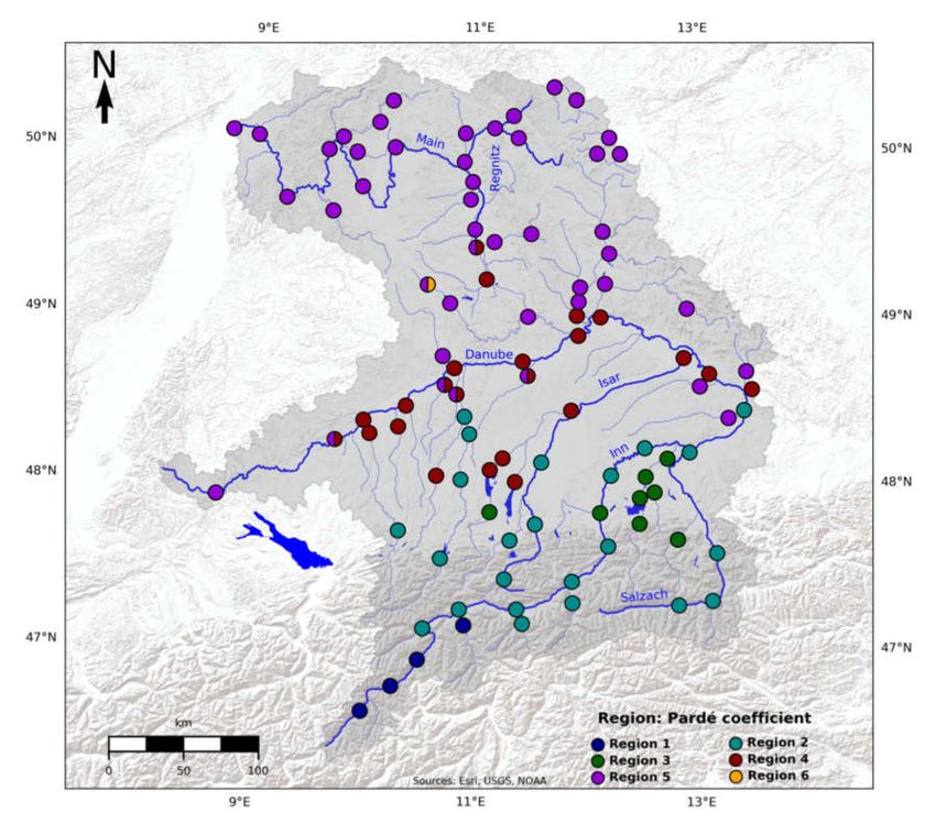
Water 2020, 12, 1599 2 of 21
runoff characteristics, as the outcome is of great interest for stakeholders and decision makers in the
affected catchments.
Generally, all hydrological analyses based on climate simulations suffer not only from the
uncertainties induced by the model uncertainty of the hydrological model, uncertainty due to the bias
correction and statistical downscaling, but also from uncertainties regarding the driving climate [28].
These climate uncertainties can be addressed to three different sources [29–31]: (1) Scenario uncertainty
occurs because the actual emissions in the future are not known but estimated within the emission
scenarios. (2) Additionally, there is model uncertainty caused by the global and regional climate
models (GCM, RCM). Though climate models may be structurally similar to each other, they differ in
spatial resolution, in the degree of detail regarding the implementation of different atmospheric and
oceanic processes and in the use of varying parametrization schemes. Therefore, climate simulations of
various GCM and RCM combinations differ though driven by the same radiative forcing and emission
scenario. (3) Internal variability is caused by non-linear dynamical processes, which are inherent to
the chaotic nature of the climate system [32]. Hence, climate simulations based on combinations of
the same GCM, RCM, radiative forcing and emission scenario will differ if the initial atmospheric
conditions of the GCM are very slightly perturbed [29,33].
Many studies regarding the impact of climate change on runoff characteristics in central Europe
have been conducted on different scales, with various climate simulations and analysis methods.
Most of these studies apply modeling chains featuring multi-model ensembles of climate simulations
to account for the climate model uncertainty [7,34,35]. Some of the studies are carried out with different
emission scenarios to address the scenario uncertainty [8,36,37]. Other experiments also set up different
hydrological models to account for the hydrological model uncertainty [38–40]. The uncertainty due to
different bias correction algorithms is addressed by Meyer et al. [41]. To our knowledge, there is no
study yet which assesses the impact of internal variability of the climate system on the runoff regime
in Europe. Champagne et al. [42] use the CRCM5-LE and WaSiM-ETH to assess the internal variability
of streamflow simulations in southern Ontario.
Other projects apply large climate model ensembles in order to model the effect of climate
change on socio-economic impacts such as heatwaves, droughts or wildfire [43,44], wind [45,46],
agriculture [47–50], storm surges [51,52] and floods [53].
Within this study, we use 50 high-resolution climate simulations from the single model initial
condition large ensemble (SMILE) CRCM5-LE to drive the hydrological model WaSiM-ETH [54]
resulting in 50 hydrological simulations, which differ only due to the internal variability of the climate
system. After calculating the Pardé coefficients in the 98 catchments of the study area for the reference
period (1981–2010), we apply a hierarchical cluster analysis on this broad database in order to classify
the 50 × 98 = 4900 regimes into six groups. Hierarchical clustering has been successfully applied
on various hydrological parameters [55]. Clustering of regimes based on observational data was
carried out by Lebiedzinski and Fürst [56] and Berhanu et al. [57]. For the six regime clusters within
this study, the change of the runoff characteristics according to the Pardé coefficient between the
reference period and the near future (2011–2040), mid future (2041–2070) and far future (2071–2099) is
analyzed. These changes are addressed to the climate change-induced seasonal shifts, which increases
and decreases in the components of the water cycle. The cluster analysis is again applied on the
hydrological simulations of the near, mid and far future in order to test whether the shifts in the runoff
characteristics of each catchment causes its regime class to change.
2. Study Area and Data
2.1. Study Area
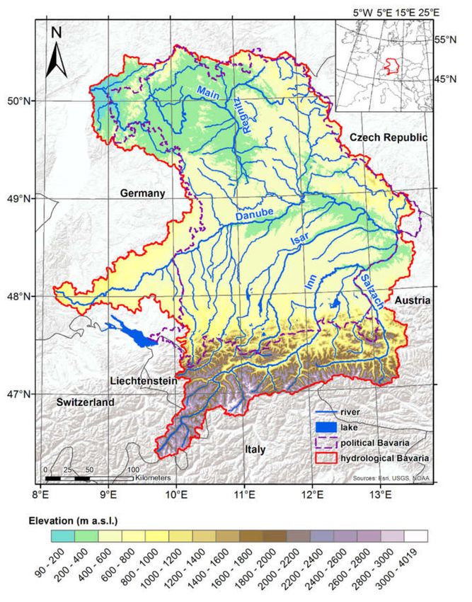
The study region covers an area of 103,201 km2 with elevations between 90 m above sea level
at Frankfurt Osthafen (Main outlet) and 4019 m above sea level at Piz Bernina (Figure 1). For the
hydrological modeling, the study area is divided into 98 sub-catchments according to the size of the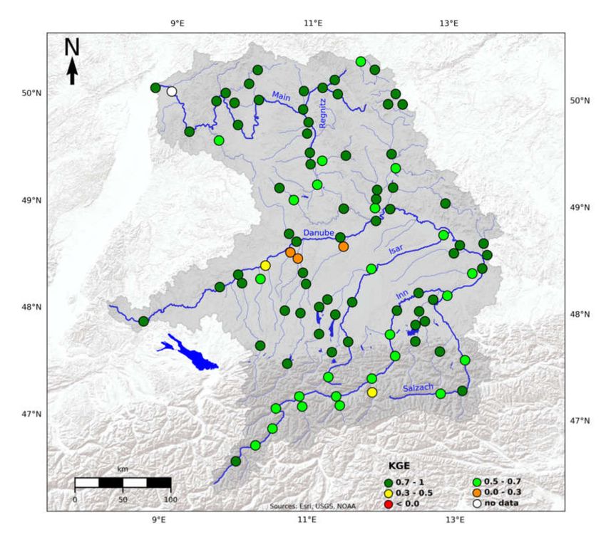
Water 2020, 12, 1599                                                                                       3 of 21

respective catchment and to its importance for water management. The whole region is referred
to as “hydrological Bavaria”, as it corresponds to the political Bavaria, but is slightly extended
according to the location of the catchments, mainly towards the west and south. Hence, also gauges in
Baden-Württemberg, Austria and Switzerland contribute to the study.

      Figure 1. Elevation of the study area [58]. The study area is marked as red line and the violet dashed
      line denotes the political border of Bavaria.

     The spatial distribution of annual precipitation is governed by the elevation, slope and exposition.
The northern and central parts of the study area between 50.5◦ N and 48◦ N show an annual precipitation
of 500–1000 mm during the reference period, whereby the low mountain ranges, such as the Fichtel
Mountains, Swabian and Franconian Jura as well as the Bavarian Forest feature annual precipitation
around 1000 mm. South of 48◦ N, precipitation is orographically enhanced due to the rising elevation
in the Alpine Foreland and Pre-Alps resulting in annual totals of 1500 up to 2500 mm at the southern
political border of Bavaria at around 47.5◦ N. South of that, the Inn catchment consists of inner-alpine
dry valleys with annual precipitation lower than 1000 mm, whereas the mountains within the Inn
catchment show values beyond 1000 mm. In the Salzach catchment, annual precipitation totals between
1000 and 2000 mm are observed. Annual air temperatures in the north of the study area are around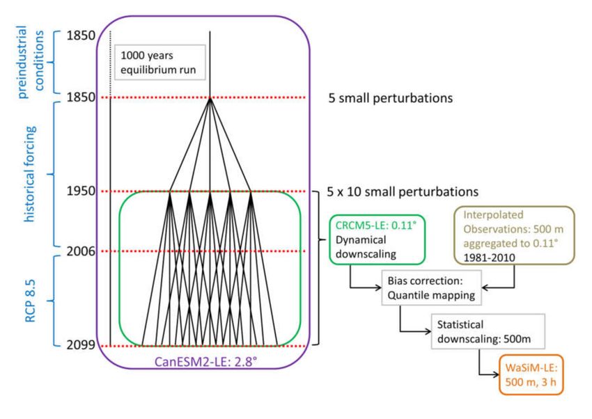
Water 2020, 12, 1599                                                                               4 of 21

10 ◦ C. Between 49.5◦ N and 47◦ N, 7–9 ◦ C are measured. In the Alps, air temperatures range from −6
to −2 ◦ C on the mountain tops and up to 8 ◦ C in the valleys.

2.2. Data
     The driving climate for this hydrological experiment is based on a large ensemble of GCM
simulations, which was performed with the Canadian Earth System Model version 2 (CanESM2) run
at ~2.8◦ spatial resolution [59,60]. This SMILE is referred to as CanESM2-LE and its setup is explained
in the following.
     After a 1000-year equilibrium run of the CanESM2 forced by preindustrial conditions featuring a
constant 284.7-ppm atmospheric CO2 concentration, random atmospheric perturbations were applied
resulting in five runs starting on 1 January 1850 [33]. These five simulations can be seen as “families”
within the large ensemble and were run until December 1949. Then, new random atmospheric
perturbations were implemented so that each of the five families separate into 10 members leading to a
pool of 50 members in sum, which are simulated until December 2005. The simulations of the five
families and the 50 members were forced with estimations of historical CO2 and non-CO2 greenhouse
gas emissions, aerosol concentrations, and land use. Furthermore, estimations of changes in solar
irradiance and in aerosol concentration due to volcano explosions are included [60]. The historical
period ends in December 2005, whereupon the simulations follow the radiative forcing from the
representative concentration pathway (RCP) 8.5 from 2006 to 2099.
     The application of the slight perturbations to the initial atmospheric state on 1 January, 1850,
and again on 1 January, 1950, leads to different climate realizations, whereby the model dynamics,
physics or structure were not changed [60]. After a few years from their initialization in 1950,
the resulting 50 simulations are assumed to be independent realizations of the modeled climate
system [33]. As the analysis period within this study starts in 1981, the variability of the 50 members
can be interpreted as internal variability [29].
     The Canadian Regional Climate Model, version 5 (CRCM5) [61,62] featuring a spatial resolution
of 0.11◦ is then applied to dynamically downscale the CanESM2-LE within 1950–2099. This RCM
SMILE is referred to as CRCM5-LE and was designed within the ClimEx project (Climate change and
hydrological extreme events–risks and perspectives for water management in Bavaria and Québec;
Munich, Germany). More details of the CanESM2-LE setup can be found in [60]. Details regarding
the downscaling as well as a validation of the CRCM5-LE against E-OBS data are presented in [33].
A comparison of the CRCM5-LE to the EURO-CORDEX (European Domain-Coordinated Regional
Climate Downscaling Experiment) multi-model ensemble is shown in [31].
     As RCMs overestimate the occurrence of drizzle [63], precipitation values below 1 mm/d are
eliminated [64]. Due to the biases of the CRCM5-LE over the study area regarding precipitation and
temperature [33], a bias correction is carried out in order to prevent the deviations from propagating in
the simulation of the water cycle [65–68]. Hence, a quantile mapping approach [69] is applied with a
three-hourly resolution to adjust all input variables, which are used for the hydrological simulations of
the WaSiM-ETH, namely precipitation, air temperature in 2 m height, surface downwelling shortwave
radiation and surface wind speed.
     After the application of a statistical downscaling resulting in a spatial resolution of 500 m,
this climate dataset drives the hydrological model WaSiM-ETH with a temporal resolution of 3 h.
The whole setup is summed up in Figure 2 and further details regarding the input data as well as the
implemented modules are presented in the Supplementary Materials. Water management structures
such as reservoirs and transition canals are implemented within the setup as far as the data are provided
by the Bavarian Agency for Environment.
     The Kling-Gupta Efficiency (KGE) [70] for the whole reference period is presented in Figure 3.
Except for the gauges of the rivers Mindel, Zusam, Schmutter and Paar in the center of the study area as
well as the alpine river Ziller, all other catchments show a good or very good agreement of observation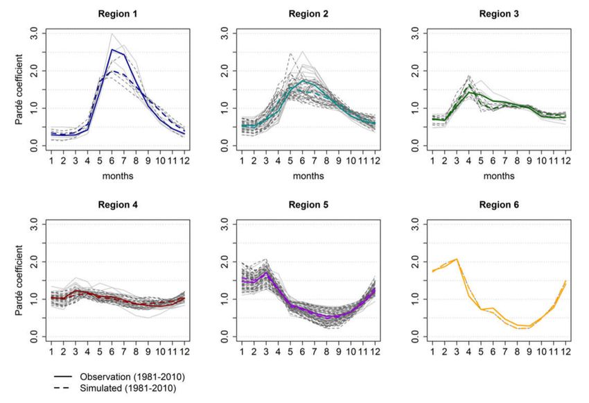
Water 2020, 12, 1599                                                                                     5 of 21

and simulation (KGE > 0.5). Due to the undercatch of mountainous precipitation gauges [41,71,72],
most alpine and pre-alpine catchments show a KGE between 0.5 and 0.7.

           Figure 2. Schematic representation of the hydrometeorological model and processing chain.

      Figure 3. KGE for all 98 catchments in hydrological Bavaria during the reference period (1981–2010).
Water 2020, 12, 1599 6 of 21
3. Methods
The hydrological regime characterized by the Pardé coefficient is governed by the climate
(temperature and precipitation), topography (elevation and exposition) and further features (land use,
soils, geology) of the catchment [2]. To evaluate the WaSiM-ETH setup for this experiment, the Pardé
coefficients are calculated for the reference period using observed runoffs and WaSiM-ETH simulations
driven by observational meteorological data. After that, monthly Pardé coefficients are calculated using
the climate model data for all 98 catchments and 50 members during the reference period resulting
in 4900 regimes. An agglomerative hierarchical clustering using the complete linkage algorithm
with Euclidean distance is applied on these 4900 regimes [56,73–75]. The number of clusters for this
algorithm is chosen by the user. As this choice is arbitrary, there are several strategies to evaluate the
number of clusters. On one hand, external criteria such as class labels (“nival”, “nivopluvial”, “pluvial”)
can be applied to compare the results of the cluster analysis to these labels, which are known to the user
beforehand [76]. On the other hand, relative criteria can be found, which evaluate different clustering
schemes, resulting by the same algorithm but with a varying number of clusters [77]. Charrad et al. [77]
provide a toolbox containing a set of different indices to evaluate clustering schemes. For this study,
we apply 27 indices, constraining them to a cluster number between 4 and 10 (see Supplementary
Materials for further details). Following the rule of majority [77], the highest number of indices, namely
10, propose six clusters. Therefore, we apply the hierarchical clustering algorithm with six clusters to
all 4900 runoff regimes.
If more than 10 regimes of the 50 total regimes per catchment are classified within a cluster,
the catchment is categorized into the respective class. This also allows a regime to belong to two or
more classes. The large ensemble of 50 members thereby contributes to the robustness of this cluster
analysis, as the application of this method using single members of the WaSiM-LE leads to differing
results. Furthermore, this methodology allows the internal variability of the climatic drivers to be
reflected in the classification of runoff regimes.
4. Results
The spatial distribution of the cluster analysis for the reference period is presented in Figure 4.
The validation of the hydrological model setup applying observational meteorological data for each
clustering region is shown in Figure 5. Thereby, a root-mean-square error (RMSE) of 0.09 on average
for all months and catchments shows sufficient agreement of the model and observations. For mainly
rainfall-driven catchments (Region 4, 5 and 6), the comparison of simulated and observed Pardé
coefficients show very good agreement. In the snowmelt-influenced catchments, the height and
position of the peak is not fully reproduced. Partially, this can be explained with the observational
meteorological data underestimating solid precipitation. The undercatch of snow can amount up to
40% for shielded gauges and 80% for unshielded gauges [71,78–80]. Grossi et al. [81] find deviations
of −15% to −66% in the northern Italian Alps. Additionally, the station density in the Alps is not
high enough [82]. As these observations influence the snowfall in the WaSiM-LE as part of the bias
correction, the snowmelt-induced runoff is underestimated as well. Apart from these deviations,
the general characteristics of each regime class are preserved.
Region 1 shows a (glacio-)nival regime with its peak in June and July (see Figure 6). The three
alpine gauges of the Inn and the Oetztaler Ache belong to this regime class, whereby the Oetztaler
Ache has its peak flow in July, which is why it is classified as glacio-nival regime [37]. Region 2 also
has its peak flow in June, but it is simulated earlier during May due to the underestimation of snowfall
and snowmelt. The regime is more balanced than the (glacio-)nival regime with a less spiky peak and
higher flows during the winter. Therefore, it is classed as a nival transition regime. The respective
catchments are located in the Pre-Alps and Alpine Foreland. Region 3 can be categorized as nivo-pluvial
regime. The peak in April is caused by a combination of rainfall and snowmelt processes, whereas
the coefficients > 1 during June to September are governed by the rain regime only. Region 4 shows
a very balanced flow regime. The catchments are located in the center of the study area near theWater 2020, 12, 1599 7 of 21
Danube. The evenness of the regime is caused by a relatively even precipitation regime with only
small influence of snowmelt during November–March. Therefore, this regime class is referred to as
pluvial (balanced). Region 5 covers almost all northern catchments. Its flow regime is governed by
the rain regime and evapotranspiration resulting in a less even monthly mean flow. The three peak
months are January, February and March, when a small amount of snowmelt adds to the rain, whereby
evapotranspiration is low. During the second half of the year this class shows a pronounced sink in the
monthly mean flows. This regime is classified as pluvial (unbalanced). The sixth cluster class consists
of 23 single regime members and is therefore only represented by the head catchment of the river
Altmühl, which belongs to class 5 and 6. The seasonal course of this regime class is similar to region 5,
with an even higher peak during January to March and a lower sink during the summer.
The cluster classes of the 4900 regimes, which are simulated by WaSiM-ETH driven by the
bias-corrected CRCM5-LE, are presented in Figure 6. Additionally, the projected change of the regional
mean of each cluster is shown for the near, mid and far future in Figure 7. The climate change-induced
shifts in the water cycle are the drivers of the regime changes (see Figure 8). The seasonal variability
of the runoff regimes in the rainfall-driven regions 3, 4, 5 and 6 is increasing for every future
period (see Figure 7). This is largely caused by increasing seasonal variability of the rainfall with
higher rainfall during November to March and less rainfall during June to September. In addition,
the evapotranspiration during May to August increases and amplifies the seasonal variability of the
mean flows (see Figure 8).
Figure 4. Six regime classes are produced by the hierarchical clustering of the 50 members for each of
the 98 catchments in hydrological Bavaria during the reference period (1981–2010).Water 2020, 12, 1599 8 of 21
Figure 5. Pardé coefficients for the reference period 1981–2010. The coefficients calculated with
measurements are marked as solid line, whereas the dashed lines represent WaSiM-ETH simulations
driven by observational meteorological data. The colored lines show the mean for each region and the
gray lines show every single catchment.
Figure 6. Pardé coefficients for the reference period 1981–2010 are calculated on the basis of all 50
members of the WaSiM-LE (gray lines). The colored lines show the regional mean for each cluster.Water 2020, 12, 1599 9 of 21
Figure 7. The regional mean Pardé coefficients during the reference period, near, mid and far future.
Shaded areas represent the range of all catchments within each cluster class.
Figure 8. Components of the water cycle simulated by the WaSiM-LE for the reference period, near,
mid and far future (same color signatures as in Figure 7). The lines represent the regional mean over
the catchments of each cluster class (weighted by the area of the catchment) and the shaded areas show
the range of all catchments within the cluster.Water 2020, 12, 1599 10 of 21
The catchments with mainly snowmelt-driven (glacio-)nival and nival transition regimes are
located in the Alps, pre-alpine regions and the Alpine Foreland, whereby the sources of these rivers are
in the Alps and Pre-Alps. Climate change-induced higher temperatures and earlier snowmelt cause
the monthly peak to occur less pronounced and earlier in the season during the mid and far future,
respectively. The relative importance of snowmelt for the monthly discharge decreases, whereas liquid
precipitation will increasingly contribute to the runoff during winter and early spring. Generally,
catchments of these both regime types will show a more balanced seasonal runoff in the future.
The monthly peak of the nivo-pluvial catchments shifts from April to March in the far future,
whereby this peak gets more intense. The normalized monthly discharge from December to March
increases in every future period, while from July to October a severe decline is found. The contribution
of snowmelt decreases by every future period, leading to a higher relative importance of rainfall.
The normalized monthly runoff of all three pluvial regime types increases in the first half of
the year by every future period and decreases in the second half of the season. These shifts can be
addressed to changes in the rainfall regime and rising evapotranspiration during May to August.
These results are consistent with several regional studies, which analyze climate change impacts on
hydrological characteristics on catchments in the Alps and Alpine Foreland [7,11,34,35,37,38,83,84].
In order to assess this impact on the categorization of the runoff regimes, the Euclidean distances
of the 4900 Pardé coefficients of the reference period to the 3 × 4900 coefficients of the near, mid and far
future are calculated. According to these distances, the regimes of the future are categorized into the
cluster classes of the reference period. The result of this classification shows if the changing climate is
causing a shift of the regime class until 2011–2040, 2041–2070 or 2071–2099 (see Figures 9–11). Table 1
summarizes the number of catchments within each cluster class.
Compared to the reference period, eight catchments will change their regime classes in the near
future. These are nival and nivo-pluvial catchments in the Alpine Foreland, where the influence
of snow decreases, which causes a shift towards a pluvial class. However, these catchments are
categorized belonging to both regime classes. This means that the change in their regimes is within the
range of natural variability for the near future.
During the mid-future, a shift in the regime class is examined for 23 catchments, which equals
to 23% of all 98 catchments (see Figure 10). The number of catchments within the snowmelt-related
classes ((glacio-)nival, nival transition, nivo-pluvial) decreases from 35 to 30. These shifting catchments
are located in the Alpine Foreland, where the importance of snowmelt declines. In this region, the
pluvial categories gain new members. In the center and north of the study area, both pluvial classes
still dominate, whereby some catchments of the Danube and near the Danube change their category
from balanced to both balanced and unbalanced.
For the far future, an even more severe shift of regime classes is found (see Figure 11). Almost all
catchments in the Alpine Foreland except for two Inn gauges turn into pluvial or nivo-pluvial regimes.
From the (glacio-)nival class, only the Oetztaler Ache remains. The former nivo-pluvial regimes
around Lake Chiemsee change to pluvial regimes. The number of catchments within the (glacio-)nival,
nival transition and nivo-pluvial classes further decreases to 22. The unbalanced pluvial regime class
(Region 5) becomes the dominant regime class with 61% of all catchments.
In sum, 42 of 98 catchments shift their regime class compared to the reference period, which amounts
to 43%. From the mid to far future, the most severe change is found. In comparison to 2041–2070,
30 catchments change their respective regime class, which equals 31%.Water 2020, 12, 1599 11 of 21
Figure 9. Hierarchical clustering of the mean regime of the 50 members of each catchment during the
near future (2011–2040) into the cluster classes of the reference period.
Figure 10. Hierarchical clustering of the mean regime of the 50 members of each catchment during the
mid-future (2041–2070) into the cluster classes of the reference period.Water 2020, 12, 1599 12 of 21
Figure 11. Hierarchical clustering of the mean regime of the 50 members of each catchment during the
far future (2071–2099) into the cluster classes of the reference period.
Table 1. Number of catchments within cluster classes for the reference (REF), near future (NF),
mid future (MF) and far future (FF) periods.
Class 1 1/2 2 2/3 2/3/4 3 3/4 3/5 4 4/5 5 5/6
REF 4 0 23 0 0 8 0 0 18 5 39 1
NF 4 0 18 1 0 6 2 0 18 6 42 1
MF 1 1 18 0 0 8 0 1 13 11 44 1
FF 1 0 14 0 1 5 0 1 5 8 60 3
As the Pardé coefficient is normalized with the annual mean, initially, these severe shifts in the
regime can be interpreted as seasonal shifts only. In order to also allow an absolute interpretation
of these shifts, the course of the mean flows for each region between 1981 and 2099 is presented
(cluster classification of the reference period; see Figure 12). The mean flow is presented relative to
the mean flow of 1981 averaged over all members for each cluster. The spread of the single-member,
single-catchment courses shows the large variability, which is introduced by the 50-member climate
ensemble. The shaded colored areas refer to the inner 80% of members aggregated for the regime
class. For the (glacio-)nival category, a constant increase in mean flow between 1981 and 2099 is
expected due to glacier melt, which equals an increase by 20% until the far future. All other four classes
reveal decreasing mean flows. The nival class shows a small decline by 6% until 2071–2099. For the
nivo-pluvial category a decrease by 17% is found. The pluvial classes show a higher variability as
they contain more catchments. The mean flow of the Region 4 pluvial class decreases by 19% and the
mean flow of the Region 5 pluvial class shows the most severe decrease of 22% until the far future.
The class of Region 6 is only represented by 23 single-member, single-catchment regimes. Their mean
flow decreases by 18% on average until 2071–2099.Water 2020, 12, 1599 13 of 21
Figure 12. Annual MQ for each region relative to the average MQ of 1981 (mean over all catchments of
the cluster). Gray lines denote every member of each catchment. The colored line shows the mean of
all members and catchments per region. The colored shaded area corresponds to the range between the
10th and 90th percentile of each cluster.
The variability of annual mean flows introduced by the spread of the 50-member large ensemble
can also be expressed with the coefficient of variation (CV). The CV is defined as the standard deviation
normalized by the mean. In Table 2, we present the CV of the mean 30-year MQ for the reference and
the three future periods, whereby the CV of all contributing catchments is averaged for the respective
region. The values illustrate that the variability of individual extreme years (Figure 12) is filtered out
by averaging the mean flows over 30 years. Nevertheless, coefficients of variation between 2% and 8%
are shown, with a steady increase in variability projected for the future periods.
Table 2. Coefficient of variation of the mean 30-year MQ within cluster classes for the reference (REF),
near future (NF), mid future (MF) and far future (FF) periods.
Region 1 Region 2 Region 3 Region 4 Region 5 Region 6
REF 4.90% 2.01% 2.73% 3.60% 5.13% 6.05%
NF 6.40% 2.80% 3.71% 4.70% 6.68% 7.12%
MF 6.84% 3.00% 4.27% 5.82% 7.26% 6.87%
FF 7.40% 3.01% 4.61% 6.35% 7.78% 7.39%
5. Discussion
5.1. Advantages of the Clustering Approach
The application of hierarchical clustering on a large ensemble of Pardé coefficients enables a robust
classification. The driving climate just differs by internal variability, and due to that also the simulated
runoff regimes vary. As the driving climate has a big impact on the runoff regime, the most extreme
members at the edges of the ensemble in terms of rainfall, snowfall and air temperature would lead to
a different categorization for some catchments. Hence, the broad database of 1500 years simulated
runoff per 30-year period ensures that individual extreme members do not distort the classification.
Furthermore, this approach allows catchments to be assigned to more than one regime category.
This shows the variability of the flow regime according to its driving climate. As hydrological systemsWater 2020, 12, 1599 14 of 21
behave non-linearly, the internal variability of the climate system leads to an internal variability within
the flow regimes. This can be represented by shared categories.
Pardé [12], Grimm ([85] for Europe) or subsequent studies (Mader et al. [86] for Austria) suggested
a categorization of regimes for different regions based on the timing and order of the monthly maximum
and minimum coefficients. Since runoff regimes represent a dynamical system [87], these kinds of
rigid categorization would lead to non-representative classification results, especially for catchments,
where the peak of mean flows is not pronounced [56].
In contrast, the agglomerative hierarchical clustering featuring the complete linkage algorithm
uses the Euclidean distance to cluster the regimes, which includes the whole course of the regime,
not only the position of the peaks. In our case, region 4 shows a mixed regime without pronounced
peaks and sinks, as it is driven by southern tributaries with nival or nivo-pluvial regimes as well as
by the rainfall regime, which directly affects the catchment. The clustering algorithm includes the
seasonal runoff information of all 12 months leading to a robust classification, which is also represented
by the spatial distribution of region 4 in Figure 4. Furthermore, the pluvial regimes of regions 5 and 6
show a similar timing of the peak and sink. The classical categorizations of Pardé [12], Grimm [85] or
Mader et al. [86] would have included both classes in one category. Though, the Euclidean distance of
regions 5 and 6 causes the hierarchical clustering algorithm to divide both classes. As region 6 shows a
very pronounced sink during July to October (Figure 6) and the mean flow in this region decreases
(Figure 12), it is important that the categorization reflects this behavior.
Moreover, the choice of the number of clusters is objectively determined by the use of the set of
indices by Charrad et al. [77]. Hence, the whole procedure of selecting the number of clusters, creating
the classes and analyzing the regime changes due to climate change are only driven by the data and
are therefore objective and generally applicable in any region of the world.
Therefore, this classification method is on the one hand more flexible than methods focusing on
the peaks only and on the other hand this method is nonarbitrary [56].
5.2. Socio-Economic Impacts of the Runoff Regime Change in Bavaria
The changes in the runoff regime impact several socio-economic sectors as well as the ecology
of the river and its surrounding areas [16]. In order to assess the ecological impact, river basins
would have to be considered individually and other factors such as changes in water temperature,
chemical composition, flood frequency and low water frequency would have to be additionally taken
into account.
Therefore, we discuss possible socio-economic impacts in the following. Generally, changes in the
hydrological regime have the potential to increase competition over water, as the availability of water
changes in terms of time and quantity [3]. Therefore, sustainable water resource management has to
adapt not only to the physical changes, which are projected within this study, but also to socio-economic
shifts in land and water use.
One of these possible changes relates to the water use for irrigation. In Bavaria, which covers
big parts of the study area, there are 93,300 forestry companies and agricultural enterprises growing
cereals, vegetables, grapes and hops, producing fodder for livestock and keeping dairy cattle and
livestock (status: 2013 [88]). During the past decades, only 1% of all agricultural land in Bavaria was
irrigated regularly and officially [89,90]. The need for irrigation was mainly dependent on the crop,
with predominantly various vegetables and potatoes being irrigated. Due to rising evapotranspiration
and less rainfall during the summer (see Figure 7), the water demand for irrigation is expected to
increase drastically [91,92]. In the study area, especially the cultivation of maize and vegetables, such as
potatoes, cabbage, carrots and onions will be affected by the decline in summer precipitation leading
to increasing irrigation demands. In the catchments north of the Danube, the dry and hot summer
of 2018 has already induced many farmers to irrigate their fields. Irrigation water is drawn from
groundwater or from riverbanks by wells, or it is directly pumped from reservoirs, lakes and rivers [88].Water 2020, 12, 1599 15 of 21
Since groundwater levels are expected to fall [93] and the mean flows during summer decrease in the
pluvial regime classes (Figure 7), there is an increasing risk of irrigation water scarcity.
Hydropower contributes 14.4%, equaling 12.2 TWh, to the power generation in Bavaria (status:
2017, [94]). Most of the hydropower plants are located at the southern tributaries to the Danube,
the Danube itself and the river Main [95]. The seasonality of the runoff regime has a big impact
on run-of-river power plants as they are dependent on the actual runoff, whereas reservoir power
plants can bridge low-flow periods by damming up water. The hydropower plants at the Main as
well as around 70% of the power plants of the Danube tributaries are run-of-river power plants [20].
As the amount of generated power can be expressed as approximately linearly dependent on the
runoff volume [20], we can include the changes in seasonality (Figure 7) and the course of mean flows
(Figure 12) to estimate the impact on seasonal hydropower power generation. For the hydropower
plants in the pluvial regions, the potential for power generation sinks severely during the second half
of the year due to lower mean flow periods. However, the hydropower plants, which are located closer
to the Alps in the nival regions, show a more balanced power generation potential in the future as
increasing rainfall and decreasing snow storage during the winter ensure an even flow seasonality.
Though, the annual power generation is projected to decrease according to the mean flows (Figure 12).
These findings tie in with the results of the study of Koch et al. [20], which focuses on the hydropower
in the Upper Danube basin.
Fossil fuel-based power plants, such as coal-, gas-, waste- and oil-fired as well as nuclear plants
also demand water in order to cool down the steam in the condenser. The biggest power plants in
the study area are located at the larger rivers, the Danube, Isar and Main. Their water demand is
dependent on the power plant utilization, but also on the meteorological conditions [21], whereby
at a constant utilization more cooling water is needed during the summer. The decline of annual
mean flows and seasonal mean flows during the second half of the year in pluvial regimes should
be considered when power plants are managed. However, due to the nuclear and coal phaseout in
Germany until 2022 and 2038 [96,97], the effect on power plant cooling due to regime changes are
unlikely to have big impact by the mid or far future.
The inland waterway transport in the study area is mainly focused on the federal waterways Main
and Danube and their interconnection, the Main-Danube canal, with a cargo handling of 6–15 Mt/a
during the last 30 years [98]. Conditions of lower flow reduce the possible maximum draught of vessels,
which thereby decrease the efficiency of inland water transport [24]. Furthermore, the risk of grounding
and collisions rises due to reduced depth and width of the fairway. The analysis of the mean flows
does not include any extreme low-flow conditions, but the trend of decreasing mean flows between
August and October at the rivers Danube and Main may cause limitations for the shipping. For all
gauges along the German federal waterways, the mean flow of August to October decreases by 21%,
25% and 44% on average until the near, mid and far future, respectively. Further analysis of extreme
low-flow events is necessary to assess the frequency and duration of periods, where navigability is not
only reduced, but severely affected or even completely restricted.
6. Conclusions
The WaSiM-LE, a large ensemble of hydrological simulations, which is driven by the regional
climate simulations of the CRCM5-LE, is used to categorize runoff regimes in hydrological Bavaria.
The application of a large ensemble for this analysis provides added value as the 50 members cover
a range of climatic internal variability representing the dynamical characteristics of runoff regimes.
This leads to a broad database of regimes per catchment and time period, which enables a robust
clustering analysis. In the study area, six regime classes are found for the reference period: (glacio-)nival,
nival (transition), nivo-pluvial, pluvial (balanced), pluvial (unbalanced) and a second, more unbalanced
pluvial class.
The CRCM5-LE featuring the high-emission scenario RCP 8.5 shows major changes in the driving
climate for all future periods. The findings of earlier snowmelt, less snowfall, more evapotranspirationWater 2020, 12, 1599 16 of 21
and a changing rainfall regime towards the future tie in with the results of other local and regional
studies. Due to these severe impacts of climate change on the water cycle, a shift of the regime
class is found for 8%, 23% and 43% of the catchments until the near, mid and far future, respectively.
Until 2070–2099, no kind of nival regime will persist in the Alpine Foreland except for two gauges of
the river Inn. The sinks during summer of all regimes north of the Alps become more pronounced for
each future period resulting in a big increase of the unbalanced pluvial region 5. This class shows a
very distinct seasonal behavior with Pardé coefficients around 0.2 during August to October in the
far future.
The change of the seasonal mean flows will be a major challenge for water management and will
have a big impact on stakeholders in the respective catchments. We discussed impacts on the water
supply for irrigation, the industrial water demand, and the navigability of waterways. Especially for
run-of-river hydropower plants located in catchments in a pluvial regime class, the more pronounced
seasonality with decreasing mean flows in the second half of the year will lead to severe losses in the
potential of power generation.
Supplementary Materials: The following refer to [99–104] and are available online at http://www.mdpi.com/
2073-4441/12/6/1599/s1, Figure S1: Median of the seasonal temperatures for the uncorrected (BC0) and bias
corrected (BC1) climate model ensemble as well as their difference (BC0–BC1), Figure S2: Median of the seasonal
precipitation for the uncorrected (BC0) and bias corrected (BC1) climate model ensemble as well as their difference
(BC0–BC1), Table S1: Data used for the WaSiM-ETH setup, Table S2: Modules applied in the WaSiM-ETH setup,
Table S3: Optimal number of clusters for 4900 Pardé coefficients chosen by 27 different indices. The indices have
been restricted to the range of four to ten cluster classes.
Author Contributions: Conceptualization, B.P.; WaSiM-ETH setup, F.W.; methodology of clustering analysis, B.P.;
software, B.P. and F.W.; validation, F.W.; formal analysis, B.P.; investigation, B.P.; resources, R.L.; data curation,
B.P., F.W.; writing—original draft preparation, B.P.; writing—review and editing, B.P., F.W. and R.L.; visualization,
B.P. and F.W.; supervision, R.L.; project administration, R.L.; funding acquisition, R.L. All authors have read and
agreed to the published version of the manuscript.
Funding: This research was funded by the Bavarian State Ministry for the Environment and Consumer
Protection. Computations with the CRCM5 and WaSiM-ETH for the ClimEx project were made on the SuperMUC
supercomputer at Leibniz Supercomputing Centre (LRZ) of the Bavarian Academy of Sciences and Humanities.
The operation of this supercomputer is funded via the Gauss Centre for Supercomputing (GCS) by the German
Federal Ministry of Education and Research and the Bavarian State Ministry of Education, Science and the Arts.
Acknowledgments: We thank all members of the ClimEx project working group for their contributions to produce
and analyze the CanESM2-LE, CRCM5-LE and WaSiM-LE. Especially, we want to thank Raul Wood for the
creation of the meteorological reference data, which was used for the bias adjustment and Magdalena Mittermeier
for the analysis of the differences between BC0 and BC1. The CRCM5 was developed by the ESCER centre of
Université du Québec a Montréal (UQAM; http://www.escer.uqam.ca) in collaboration with Environment and
Climate Change Canada. We acknowledge Environment and Climate Change Canada’s Canadian Centre for
Climate Modelling and Analysis for executing and making available the CanESM2 Large Ensemble simulations
used in this study, and the Canadian Sea Ice and Snow Evolution Network for proposing the simulations. We also
thank the developer of WaSiM-ETH (http://www.wasim.ch/de/), Jörg Schulla for his support.
Conflicts of Interest: The authors declare no conflict of interest. The funders had no role in the design of the
study; in the collection, analyses, or interpretation of data; in the writing of the manuscript, or in the decision to
publish the results.
References
1. Messerli, B.; Viviroli, D.; Weingartner, R. Mountains of the World: Vulnerable Water Towers for the 21st
Century. In Special Report Number 13. The Royal Colloquium: Mountain Areas: A Global Resource; Springer:
Berlin/Heidelberg, Germany, 2004; pp. 29–34. [CrossRef]
2. Bormann, H. Runoff regime changes in German rivers due to climate change. Erdkunde 2010, 64, 257–279.
[CrossRef]
3. Strasser, U.; Marke, T.; Braun, L.; Escher-Vetter, H.; Juen, I.; Kuhn, M.; Maussion, F.; Mayer, C.; Nicholson, L.;
Niedertscheider, K.; et al. The Rofental: A high Alpine research basin (1890 m–3770 m a.s.l.) in the Ötztal
Alps (Austria) with over 150 years of hydro-meteorological and glaciological observations. Earth Syst. Sci.
Data 2018, 10, 151–171. [CrossRef]Water 2020, 12, 1599 17 of 21
4. Ionita, M.; Badaluta, C.-A.; Scholz, P.; Chelcea, S. Vanishing river ice cover in the lower part of the Danube
basin—Signs of a changing climate. Sci. Rep. 2018, 8, 7948. [CrossRef] [PubMed]
5. Beniston, M. Impacts of climatic change on water and associated economic activities in the Swiss Alps.
J. Hydrol. 2012, 412–413, 291–296. [CrossRef]
6. Gobiet, A.; Kotlarski, S.; Beniston, M.; Heinrich, G.; Rajczak, J.; Stoffel, M. 21st century climate change in the
European Alps—A review. Sci. Total Environ. 2014, 493, 1138–1151. [CrossRef]
7. Milano, M.; Reynard, E.; Bosshard, N.; Weingartner, R. Simulating future trends in hydrological regimes in
Western Switzerland. J. Hydrol. Reg. Stud. 2015, 4, 748–761. [CrossRef]
8. Stagl, J.; Hattermann, F. Impacts of Climate Change on the Hydrological Regime of the Danube River and Its
Tributaries Using an Ensemble of Climate Scenarios. Water 2015, 7, 6139–6172. [CrossRef]
9. Rojas, R.; Feyen, L.; Bianchi, A.; Dosio, A. Assessment of future flood hazard in Europe using a large ensemble
of bias-corrected regional climate simulations. J. Geophys. Res. 2012, 117, D17109. [CrossRef]
10. Schneider, C.; Laizé, C.L.R.; Acreman, M.C.; Flörke, M. How will climate change modify river flow regimes
in Europe? Hydrol. Earth Syst. Sci. 2013, 17, 325–339. [CrossRef]
11. Köplin, N.; Viviroli, D.; Schädler, B.; Weingartner, R. How does climate change affect mesoscale catchments
in Switzerland?—A framework for a comprehensive assessment. Adv. Geosci. 2010, 27, 111–119. [CrossRef]
12. Pardé, M. Fleuves et Rivières; Armand Colin: Paris, France, 1933; p. 224.
13. Gaudry, M.M.C.; Gutknecht, D.; Parajka, J.; Perdigão, R.A.P.; Blöschl, G. Seasonality of runoff and precipitation
regimes along transects in Peru and Austria. J. Hydr. Hydromech. 2017, 65, 347–358. [CrossRef]
14. Cañedo-Argüelles, M.; Kefford, B.J.; Piscart, C.; Prat, N.; Schäfer, R.B.; Schulz, C.-J. Salinisation of rivers:
An urgent ecological issue. Environ. Pollut. 2013, 173, 157–167. [CrossRef] [PubMed]
15. Poff, N.L.; Allan, J.D.; Bain, M.B.; Karr, J.R.; Prestegaard, K.L.; Richter, B.D.; Sparks, R.E.; Stromberg, J.C.
The Natural Flow Regime. A paradigm for river conservation and restoration. BioScience 1997, 47, 769–784.
[CrossRef]
16. Poff, N.L.; Zimmerman, J.K.H. Ecological responses to altered flow regimes: A literature review to inform
the science and management of environmental flows. Freshw. Biol. 2010, 55, 194–205. [CrossRef]
17. Bruckerhoff, L.A.; Leasure, D.R.; Magoulick, D.D. Flow–ecology relationships are spatially structured and
differ among flow regimes. J. Appl. Ecol. 2019, 56, 398–412. [CrossRef]
18. Schleuter, M. Computing the degradation of riparian floodplains by means of a water-level difference curve.
Hydrol. Wasserbewirtsch. 2010, 54, 360–367.
19. Gaudard, L.; Romerio, F. The future of hydropower in Europe: Interconnecting climate, markets and policies.
Environ. Sci. Policy 2014, 37, 172–181. [CrossRef]
20. Koch, F.; Prasch, M.; Bach, H.; Mauser, W.; Appel, F.; Weber, M. How Will Hydroelectric Power Generation
Develop under Climate Change Scenarios? A Case Study in the Upper Danube Basin. Energies 2011, 4,
1508–1541. [CrossRef]
21. Koch, H.; Vögele, S. Dynamic modelling of water demand, water availability and adaptation strategies for
power plants to global change. Ecol. Econ. 2009, 68, 2031–2039. [CrossRef]
22. Bär, R.; Rouholahnejad, E.; Rahman, K.; Abbaspour, K.C.; Lehmann, A. Climate change and agricultural
water resources: A vulnerability assessment of the Black Sea catchment. Environ. Sci. Policy 2015, 46, 57–69.
[CrossRef]
23. Jonkeren, O.; Rietveld, P.; van Ommeren, J.; te Linde, A. Climate change and economic consequences for
inland waterway transport in Europe. Reg. Environ. Chang. 2014, 14, 953–965. [CrossRef]
24. Nilson, E.; Krahe, P. Navigation on the rhine river and climate change. Geogr. Rundsch. 2013, 65, 26–33.
25. Stoelzle, M.; Blauhut, V.; Kohn, I.; Weiler, M.; Stahl, K. Niedrigwasser in Süddeutschland Analysen, Szenarien und
Handlungsempfehlungen; Arbeitskreis KLIWA, Ed.; Bayerisches Landesamt für Umwelt: Hof, Germany, 2018;
p. 95.
26. Ehsani, N.; Vörösmarty, C.J.; Fekete, B.M.; Stakhiv, E.Z. Reservoir operations under climate change: Storage
capacity options to mitigate risk. J. Hydrol. 2017, 555, 435–446. [CrossRef]
27. Fatichi, S.; Rimkus, S.; Burlando, P.; Bordoy, R.; Molnar, P. High-resolution distributed analysis of climate and
anthropogenic changes on the hydrology of an Alpine catchment. J. Hydrol. 2015, 525, 362–382. [CrossRef]
28. Willkofer, F.; Schmid, F.-J.; Komischke, H.; Korck, J.; Braun, M.; Ludwig, R. The impact of bias correcting
regional climate model results on hydrological indicators for Bavarian catchments. J. Hydrol. Reg. Stud. 2018,
19, 25–41. [CrossRef]Water 2020, 12, 1599 18 of 21
29. Deser, C.; Phillips, A.; Bourdette, V.; Teng, H. Uncertainty in climate change projections: The role of internal
variability. Clim. Dyn. 2012, 38, 527–546. [CrossRef]
30. Hawkins, E.; Sutton, R. The potential to narrow uncertainty in regional climate predictions. Bull. Am.
Meteorol. Soc. 2009, 90, 1095–1108. [CrossRef]
31. Von Trentini, F.; Leduc, M.; Ludwig, R. Assessing natural variability in RCM signals: Comparison of a multi
model EURO-CORDEX ensemble with a 50-member single model large ensemble. Clim. Dyn. 2019, 53,
1963–1979. [CrossRef]
32. Martel, J.-L.; Mailhot, A.; Brissette, F.; Caya, D. Role of Natural Climate Variability in the Detection of
Anthropogenic Climate Change Signal for Mean and Extreme Precipitation at Local and Regional Scales.
J. Clim. 2018, 31, 4241–4263. [CrossRef]
33. Leduc, M.; Mailhot, A.; Frigon, A.; Martel, J.-L.; Ludwig, R.; Brietzke, G.; Giguère, M.; Brissette, F.; Turcotte, R.;
Braun, M.; et al. The ClimEx Project: A 50-Member Ensemble of Climate Change Projections at 12-km
Resolution over Europe and Northeastern North America with the Canadian Regional Climate Model
(CRCM5). J. Appl. Meteorol. Clim. 2019, 58, 663–693. [CrossRef]
34. Coppola, E.; Raffaele, F.; Giorgi, F. Impact of climate change on snow melt driven runoff timing over the
Alpine region. Clim. Dyn. 2018, 51, 1259–1273. [CrossRef]
35. Farinotti, D.; Usselmann, S.; Huss, M.; Bauder, A.; Funk, M. Runoff evolution in the Swiss Alps: Projections
for selected high-alpine catchments based on ENSEMBLES scenarios. Hydrol. Process. 2012, 26, 1909–1924.
[CrossRef]
36. Döll, P.; Schmied, H.M. How is the Impact of Climate Change on River Flow Regimes Related to the Impact on Mean
Annual Runoff? A Global-Scale Analysis; IOP Publishing Ltd: Bristol, UK, 2012; Volume 7. [CrossRef]
37. Hanzer, F.; Förster, K.; Nemec, J.; Strasser, U. Projected cryospheric and hydrological impacts of 21st century
climate change in the Ötztal Alps (Austria) simulated using a physically based approach. Hydrol. Earth Syst.
Sci. 2018, 22, 1593–1614. [CrossRef]
38. Addor, N.; Rössler, O.; Köplin, N.; Huss, M.; Weingartner, R.; Seibert, J. Robust changes and sources of
uncertainty in the projected hydrological regimes of Swiss catchments. Water Resour. Res. 2014, 50, 7541–7562.
[CrossRef]
39. Ludwig, R.; May, I.; Turcotte, R.; Vescovi, L.; Braun, M.; Cyr, J.-F.; Fortin, L.-G.; Chaumont, D.; Biner, S.;
Chartier, I.; et al. The role of hydrological model complexity and uncertainty in climate change impact
assessment. Adv. Geosci. 2009, 21, 63–71. [CrossRef]
40. Velázquez, J.A.; Schmid, J.; Ricard, S.; Muerth, M.; Gauvin St-Denis, B.; Minville, M.; Chaumont, D.; Caya, D.;
Ludwig, R.; Turcotte, R. An ensemble approach to assess hydrological models’ contribution to uncertainties
in the analysis of climate change impact on water resources. Hydrol. Earth Syst. Sci. 2013, 17, 565–578.
[CrossRef]
41. Meyer, J.; Kohn, I.; Stahl, K.; Hakala, K.; Seibert, J.; Cannon, A.J. Effects of univariate and multivariate
bias correction on hydrological impact projections in alpine catchments. Hydrol. Earth Syst. Sci. 2019, 23,
1339–1354. [CrossRef]
42. Champagne, O.; Arain, A.; Leduc, M.; Coulibaly, P.; McKenzie, S. Future shift in winter streamflow modulated
by internal variability of climate in southern Ontario. Hydrol. Earth Syst. Sci. Discuss. 2019, 1–30. [CrossRef]
43. Shiogama, H.; Hirata, R.; Hasegawa, T.; Fujimori, S.; Ishizaki, N.N.; Chatani, S.; Watanabe, M.; Mitchell, D.;
Lo, Y.T.E. Historical and future anthropogenic warming effects on droughts, fires and fire emissions of CO2
and PM2.5 in equatorial Asia when 2015-like El Niño events occur. Earth Syst. Dynam. 2020, 11, 435–445.
[CrossRef]
44. Barcikowska, M.J.; Muñoz, Á.G.; Weaver, S.J.; Russo, S.; Wehner, M. On the potential impact of a half-degree
warming on cold and warm temperature extremes in mid-latitude North America. Environ. Res. Lett. 2019,
14, 124040. [CrossRef]
45. Ohba, M. The Impact of Global Warming on Wind Energy Resources and Ramp Events in Japan. Atmosphere
2019, 10, 265. [CrossRef]
46. Hosking, J.S.; MacLeod, D.; Phillips, T.; Holmes, C.R.; Watson, P.; Shuckburgh, E.F.; Mitchell, D.M. Changes
in European wind energy generation potential within a 1.5 ◦ C warmer world. Environ. Res. Lett. 2018, 14,
054032. [CrossRef]Water 2020, 12, 1599 19 of 21
47. Iizumi, T.; Shiogama, H.; Imada, Y.; Hanasaki, N.; Takikawa, H.; Nishimori, M. Crop production losses
associated with anthropogenic climate change for 1981–2010 compared with preindustrial levels. Int. J.
Climatol. 2018, 38, 5405–5417. [CrossRef]
48. Schleussner, C.F.; Deryng, D.; Müller, C.; Elliott, J.; Saeed, F.; Folberth, C.; Liu, W.; Wang, X.; Pugh, T.A.M.;
Thiery, W.; et al. Crop productivity changes in 1.5 ◦ C and 2 ◦ C worlds under climate sensitivity uncertainty.
Environ. Res. Lett. 2018, 13, 064007. [CrossRef]
49. Gaupp, F.; Hall, J.; Mitchell, D.; Dadson, S. Increasing risks of multiple breadbasket failure under 1.5 and
2 ◦ C global warming. Agric. Syst. 2019, 175, 34–45. [CrossRef]
50. Faye, B.; Webber, H.; Naab, J.B.; MacCarthy, D.S.; Adam, M.; Ewert, F.; Lamers, J.P.A.; Schleussner, C.-F.;
Ruane, A.; Gessner, U.; et al. Impacts of 1.5 versus 2.0 ◦ C on cereal yields in the West African Sudan Savanna.
Environ. Res. Lett. 2018, 13, 034014. [CrossRef]
51. Mohit, M.A.A.; Yamashiro, M.; Hashimoto, N.; Mia, M.B.; Ide, Y.; Kodama, M. Impact Assessment of a Major
River Basin in Bangladesh on Storm Surge Simulation. J. Mar. Sci. Eng. 2018, 6, 99. [CrossRef]
52. Mori, N.; Shimura, T.; Yoshida, K.; Mizuta, R.; Okada, Y.; Fujita, M.; Khujanazarov, T.; Nakakita, E. Future
changes in extreme storm surges based on mega-ensemble projection using 60-km resolution atmospheric
global circulation model. Coast. Eng. J. 2019, 61, 295–307. [CrossRef]
53. Uhe, P.F.; Mitchell, D.M.; Bates, P.D.; Sampson, C.C.; Smith, A.M.; Islam, A.S. Enhanced flood risk with 1.5 ◦ C
global warming in the Ganges–Brahmaputra–Meghna basin. Environ. Res. Lett. 2019, 14, 074031. [CrossRef]
54. Schulla, J. Model Description WaSiM (Water Balance Simulation Model); Hydrology Software Consulting J.
Schulla: Zürich, Switzerland, 2012; p. 305.
55. Olden, J.D.; Reidy Liermann, C.A.; Pusey, B.J.; Kennard, M.J. Protocols for Hydrologic Classification and a
Review of Australian Applications. In Ecohydrological regionalisation of Australia: A Tool for Management and
Science; Land & Water Australia: Canberra, Australia, 2009; pp. 1–28.
56. Lebiedzinski, K.; Fürst, J. Entwicklung der alpinen Abflussregime in Österreich im Zeitraum 1961–2010.
Österr. Wasser Abfallw. 2018, 70, 474–484. [CrossRef]
57. Berhanu, B.; Seleshi, Y.; Demisse, S.S.; Melesse, A.M. Flow Regime Classification and Hydrological
Characterization: A Case Study of Ethiopian Rivers. Water 2015, 7, 3149–3165. [CrossRef]
58. Copernicus Land Monitoring Service—EU-DEM. Available online: https://www.eea.europa.eu/data-and-
maps/data/copernicus-land-monitoring-service-eu-dem (accessed on 24 October 2019).
59. Arora, V.K.; Scinocca, J.F.; Boer, G.J.; Christian, J.R.; Denman, K.L.; Flato, G.M.; Kharin, V.V.; Lee, W.G.;
Merryfield, W.J. Carbon emission limits required to satisfy future representative concentration pathways of
greenhouse gases. Geophys. Res. Lett. 2011, 38, L05805. [CrossRef]
60. Fyfe, J.C.; Derksen, C.; Mudryk, L.; Flato, G.M.; Santer, B.D.; Swart, N.C.; Molotch, N.P.; Zhang, X.; Wan, H.;
Arora, V.K.; et al. Large near-term projected snowpack loss over the western United States. Nat. Comm. 2017,
8, 14996. [CrossRef]
61. Martynov, A.; Laprise, R.; Sushama, L.; Winger, K.; Šeparović, L.; Dugas, B. Reanalysis-driven climate
simulation over CORDEX North America domain using the Canadian Regional Climate Model, version 5:
Model performance evaluation. Clim. Dyn. 2013, 41, 2973–3005. [CrossRef]
62. Šeparović, L.; de Elía, R.; Laprise, R. Impact of spectral nudging and domain size in studies of RCM response
to parameter modification. Clim. Dyn. 2012, 38, 1325–1343. [CrossRef]
63. Dai, A. Precipitation Characteristics in Eighteen Coupled Climate Models. J. Clim. 2006, 19, 4605–4630.
[CrossRef]
64. Kjellström, E.; Boberg, F.; Castro, M.; Christensen, J.H.; Nikulin, G.; Sánchez, E. Daily and monthly
temperature and precipitation statistics as performance indicators for regional climate models. Clim. Res.
2010, 44, 135–150. [CrossRef]
65. Ehret, U.; Zehe, E.; Wulfmeyer, V.; Warrach-Sagi, K.; Liebert, J. “Should we apply bias correction to global
and regional climate model data?”. Hydrol. Earth Syst. Sci. 2012, 16, 3391–3404. [CrossRef]
66. Maraun, D. Bias Correcting Climate Change Simulations—A Critical Review. Curr. Clim. Change Rep. 2016,
2, 211–220. [CrossRef]
67. Muerth, M.J.; Gauvin St-Denis, B.; Ricard, S.; Valázquez, J.A.; Schmid, J.; Minvie, M.; Caya, D.; Chaumont, D.;
Ludwig, R.; Turcotte, R. On the need for bias correction in regional climate scenarios to assess climate change
impacts on river runoff. Hydrol. Earth Syst. Sci. 2013, 17, 1189–1204. [CrossRef]You can also read